Exact filtering and smoothing in short or long memory stochastic switching systems

HAL Id: hal-00408868

https://hal.archives-ouvertes.fr/hal-00408868

Submitted on 3 Aug 2009

HAL is a multi-disciplinary open access

archive for the deposit and dissemination of

sci-entific research documents, whether they are

pub-lished or not. The documents may come from

teaching and research institutions in France or

abroad, or from public or private research centers.

L’archive ouverte pluridisciplinaire HAL, est

destinée au dépôt et à la diffusion de documents

scientifiques de niveau recherche, publiés ou non,

émanant des établissements d’enseignement et de

recherche français ou étrangers, des laboratoires

publics ou privés.

stochastic switching systems

Wojciech Pieczynski, Noufel Abbassi

To cite this version:

Wojciech Pieczynski, Noufel Abbassi. Exact filtering and smoothing in short or long memory stochastic

switching systems. IEEE International Workshop on MACHINE LEARNING FOR SIGNAL

PRO-CESSING, Sep 2009, Grenoble, France. �hal-00408868�

Abstract— Let X be a hidden real stochastic chain, R be a

discrete finite Markov chain, Y be an observed stochastic chain. In this paper we address the problem of filtering and smoothing in the presence of stochastic switches where the problem is to recover both R and X from Y. In the classical conditionally Gaussian state space models, exact computing with polynomial complexity in the time index is not feasible and different approximations are used. Different alternative models, in which the exact calculations are feasible, have been recently proposed since 2008. The core difference between these models and the classical ones is that the couple (R, Y) is a Markov one in the recent models, while it is not in the classical ones. Another extension deals with the case in which the observed chain Y is not necessarily Markovian conditionally on (X, R) and, in particular, the long-memory distributions can be considered. The aim of this paper is to show that, in the context of these different recent models, it is possible to calculate any moments of the posterior marginal distribution, which makes it feasible to know these distributions with any desired precision.

I. INTRODUCTION et ₁N ( ₁,..., _N) X X X = , ₁N ( ₁,..., _N) R R R = , and ) ..., , ( ₁ 1 N N _{Y Y}

Y = be three sequences of random variables. Each X and _n Y takes its values from _n R , while each R _n takes its values from a finite set Ω=

{

λ1,...,λ_K

}

. Let us notice that the proposed study is likely to be extended to N

X₁ and N

Y₁ taking their values in _{R and} q _{R , respectively;} m

however, we keep R for the sake of simplicity. The sequences _XN

1 and N

R₁ are hidden and the sequence _YN 1 is

observed. We deal with two classical problems, which are the “filtering” problem and the “smoothing” one. The formulation of these problems considered in the present paper will be, respectively:

(F) : Computation of ( 1) n n y r p and [ , 1] n n nr y X E with

complexity polynomial in time; (S) : Computation of ( ₁N) n y r p and [ , ₁N] n nr y X E with

complexity polynomial in time.

Let us consider a simple classical conditionally Gaussian state space model, which consists of considering that _RN

1 is a

Markov chain and, roughly speaking, (_X1N,_Y1N) _{is the}

Manuscript received April, 15, 2009.

W. Pieczynski and N. Abbassi are with Telecom SudParis, Evry, 91 000 France (e-mail: {wojciech.pieczynski, noufel.abbassi}@it-sudparis.eu).

classical linear system conditionally on _RN

1 . This is

summarized in the following: _RN

1 is a Markov chain; (1)

X_n+1=F_n(R_n)X_n+G_n(R_n)W_n; (2) Y_n=H_n(R_n)X_n+J_n(R_n)Z_n, (3) where X , ₁ W , …, ₁ W , _N Z , …, ₁ Z are independent _N (conditionally on N

R1 ) Gaussian variables, and F1(R1), …,

) ( _N N R F , H₁(R₁), …, H_N(R_N), G₁(R₁), …, G_N(R_N), ) ( ₁ 1 R

J , …, J_N(R_N) are real numbers depending on switches (R_n), and (2), (3) hold for each n=1, …, for each N . Such models are of interest in numerous situations [2], [3], [12], among others. However, it has been well known since [13] that the exact filtering and smoothing are not feasible with linear - or even polynomial - complexity in time in such models, and different approximations must be used. Many papers deal with this approximation problem and a rich bibliography can be seen in [1]-[3], [12].

To remedy this impossibility of exact computation different models have been recently proposed in [9]. These models, whose general idea is to consider the independence of _XN

1

and N

Y₁ conditionally on N

R₁ , lead to exact filtering and smoothing. Two kinds of extensions of these models have then been proposed. The first one, called “Markov marginal switching hidden model” (MMSHM [10]), verifies:

(_R1N,_Y1N) _{is a Markov chain; (4)} X_n+1=F_n+1(R_n+1,Y_n+1)X_n+G_n+1(R_n+1)W_n+1, (5) where F_n(r_n,y_n), G_n(r_n) are real numbers depending on

) ,

(r_n y_n , and W , …, ₁ W are independent centered real _N random variables such that W is independent from _n (_R1N,_Y1N) for each n=1, …, N . In the second one, proposed in [11], the Markov chain ( ₁N, ₁N)

Y

R is replaced by a “partially” Markov Gaussian chain recently introduced in [8], and (5) is kept. Both problems (F) and (S) can still be solved using these two models without any approximation.

The aim of this paper is to show that the calculations proposed in [10], [11] can be extended to calculations of

] , ) [( ₁n n k n r y X E and [( ) , ₁N] n k n r y X E , where k is an arbitrary positive integer. In addition, we consider a third

Exact filtering and smoothing in short or long memory stochastic

switching systems

Wojciech Pieczynski and Noufel Abbassi

model, in which the switching chain _RN

1 has a semi-Markov

distribution. This gives the moments of the distributions ) , ( ₁n n nr y x p and ( , ₁N) n nr y x

p , which means that these distributions can be known with any desired precision.

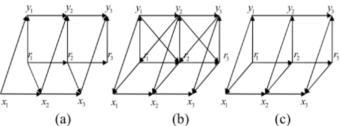
The oriented dependence graphs of the models (1)-(3), (4)-(5), and the “partially” Markov model (12)-(13) - which will be specified below - are given in Figure 1.

1 r r2 r3 1 x x₂ x3 x3 1 r r2 r3 1 x x2 1 y y2 y3 1 y y2 y3 1 r r2 r3 1 x x2 x3 1 y y2 y3 (a) (b) (c)

Fig. 1. (a): classical model (1)-(3), (b): short memory triplet Markov model (4)-(5) ; (c): long memory triplet partially Markov model.

The organization of the paper is the following. The next section is devoted to the MMSHM models, while the “hidden Markov switching conditionally linear model” (HMSCLM) models are dealt with in section three. The semi-Markov switching models are addressed in section four, and some experiments are provided in section five. The sixth section contains some conclusions.

II. TRIPLET SHORT MEMORY MARKOV MODELS

A. Filtering in a Short Memory Model

Let us consider the MMSHM model defined with (4)-(5). The computations of ( ₁n) n y r p and [( ) , ₁n] n m n r y X E are

specified in the following Lemma 1 and Proposition 1, respectively.

Lemma 1

Let us consider a triplet Markov chain (TMM) ) , , ( 1 1 1 N N N Y R X verifying (4)-(5). Then ( 1) 1 1 + + n n y r p is given from ( ₁n) ny r p by

∑∑

∑

+ + + + + + + + + = 1 ) , , ( ) , ( ) ( ) , , ( ) , ( ) ( ) ( 1 1 1 1 1 1 1 1 1 1 1 n n n r r n n n n n n n n n r n n n n n n n n n n n y r r y p y r r p y r p y r r y p y r r p y r p y r p (6) Proof We have = = + + + + +

∑

) ( ) , , ( ) ( 1 1 1 1 1 1 1 1 n n r n n n n n n y y p y y r r p y r p n ) ( ) , , ( ) , ( ) ( 1 1 1 1 1 1 n n r n n n n n n n n n y y p y r r y p y r r p y r p n + + + +

∑

, and = =

∑∑

+ + + + 1 ) , , ( ) ( _{1 1 1 1 1} n n r r n n n n n n y p r r y y y p

∑∑

+ + + + 1 ) , , ( ) , ( ) ( _{1 1 1 1} n n r r n n n n n n n n ny pr r y p y r r y r

p , which ends the

proof.

Proposition 1

Let us consider a TMM (_X1N,_R1N,_Y1N) _{defined with (4)-(5).} Let Ck (k!)/(j!)(k j)!

j = − .

For each natural number m>0, and each k=1, …, m , the conditional expectation [( ) , 1] 1 1 1 + + + n n k n r y X

E is given from the conditional expectations [ , 1] n n nr y X E , [( ) , 1] 2 n n n r y X E ,…, ] , ) [( ₁n n k n r y X E by ]) ) [( )] ( [ ] , ) [( )] , ( [ ( ] , ) [( 1 1 1 0 1 1 1 1 1 1 1 1 1 1 i k n i k n n k i k k i n n i n i n n n k i n n k n W E r G C y r X E y r F C y r X E − + − + + − = + + + + + + + +

∑

+ = = (7) = + +, ] ) [( 1 1 1 n n i n r y X E

∑

₊ + n r n n n n n i n r y p r r y X E[( ) , ] ( , 1] 1 1 1 , (8) and = + +, ) ( 1 1 1 n n nr y r p

∑

+ + n r n n n n n n n n n n y r r p y r y r r p y r p ) , ( ) ( ) , ( ) ( 1 1 1 1 . (9)

As a consequence, for each fixed natural number m>0, ] , ) [( 1 1 1 1 + + + n n k n r y X

E is computable with complexity polynomial in time.

Proof

Let m>0, and let 1≤k≤m. According to (5) we have

= + = + + + + + + + n n n n n n n k k n F R Y X G R W X ) ( ( , ) ( ) ) ( _{1 1 1 1 1 1 1}

∑

= − + − + + − + + + + k i i k n i k n n k i k i n i n n n k i F R Y X C G r W C 0 1 1 1 1 1 1( , )]( ) [ ( )] ( ) ) [ .

Taking the expectation of k n X ) ( ₊₁ conditional on ) , ( ) , ( 1 1 1 1 1 1 + + + + = n n n n Y r y

R , and taking into account the fact that the independence of W_n+1 from ( , 1)

1 1 + + n n Y R implies ] ) [( ] , ) [( 1 ₁ 1 1 1 i n n n i n r y E W W E _{+ +} + = ₊ , we may write: = + + +) , ] [( 1 1 1 1 n n k n r y X E

∑

= + + + + + + k i n n i n i n n n k i F r y E X r y C 0 1 1 1 1 1 1( , )] [( ) , ] [ ( ]) ) [( )] ( [ 1 1 1 i k n i k n n k i k G r E W C + − − + + − + , which is (7). Besides we have:

= =

∑

+ + + + + + n r n n n n n n i n n n i n r y E X r r y p r r y X E[( ) , ] [( ) , , ] ( , 1] 1 1 1 1 1 1 1 1

∑

+ + n r n n n n n i n r y p r r y X E[( ) , ] ( , 1] 1 1

1 , the last equality being due

to the independence of X and _n (R_n+1,Y_n+1) conditionally on )

, ( ₁n

nY

R (see the dependence graph (b), Figure 1). Thus (8) is verified. Finally, as R is independent from _n Y_n+1 conditionally on ( ₁, ₁n) n Y R₊ , we have ( +, +)= 1 1 1 n n nr y r p = = ( +1, 1) n n nr y r p =

∑

+ + n r n n n n n n y r r p y r r p ) , ( ) , ( 1 1 1 1

∑

+ + n r n n n n n n n n r r p y r r r p y r p ) ( ) ( ) ( ) ( 1 1 1 1 ,

which is (9) and ends the proof.

B. Smoothing in a Short Memory Model

Let us consider a TMM (X,R,Y) defined with (4)-(5), and let m>0 be a natural fixed number. The problem in this section is to calculate ( ₁N) ny r p and [( ) , ₁N] n k n r y X E for

each n=1, …, N . We can state the following results.

Lemma 2

Let us consider a TMM (_X1N,_R1N,_Y1N) _{verifying (4)-(5). The} probabilities ( ₁N) ny r p , ( ₁ , ₁N) n n r y r p ₊ , and ( ₁, ₁N) n nr y r p ₊ are computable with complexity linear in time.

Proof As (_R1N,_Y1N) _{is a Markov chain, ( )} 1 N ny r p and ) , ( _{1 1}N n n r y r

p ₊ are computable (see [8]); then ( ₁, ₁N)

n nr y r p ₊ is computed with (9). Proposition 2

Let us consider a TMM (X,R,Y) defined with (4)-(5). For each natural number m>0, and each k=1, …, m , the conditional expectation [( ₁) ₁, ₁N] n k n r y X E _{+ +} is given from ] , [ ₁N n nr y X E , [( )2 , ₁N] n n r y X E ,…, [( ) , ₁N] n k n r y X E by = + +) , ] [( _{1 1 1}N n k n r y X E

∑

= + + + + + k i N n i n i n n n k i F r y E X r y C 0 1 1 1 1 1( , )] [( ) , ] [ ( ]) ) [( )] ( [ _{1 1 1} ki n i k n n k i k G r E W C_{− + +} − ₊ − + , (10) with Ck (k!)/(j!)(k j)! j = − and = +, ] ) [( _{1 1}N n i n r y X E

∑

₊ n r N n n N n i n r y p r r y X E[( ) , ₁] ( ₁, ₁ ], (11)

As a consequence, for each fixed natural number k>0, ] , ) [( ₁N n k n r y X

E is computable with complexity polynomial in time.

Proof

To show (10), we have by assumption (5)

= + = + + + + + + + k n n n n n n n k n F R Y X G R W X ) ( ( , ) ( ) ) ( 1 1 1 1 1 1 1

∑

= − + − + + − + + + + k i i k n i k n n k i k i n i n n n k i F R Y X C G r W C 0 1 1 1 1 1 1( , )]( ) [ ( )] ( ) ) [ ( .

Taking the expectation of both sides conditional on ) , ( ) , ( 1 1 1 1 N n N n Y r y

R+ = + , and using the fact that the noise Wn+1

is independent from ( ₁, ₁N)

n Y

R+ , we have (10).

To show (11), we classically write ( +1, 1)= N n nr y x p =

∑

+ n r N n n n r r y x p( , ₁, ₁)

∑

_{+ +} = n r N n n N n n nr r y p r r y x p( , ₁, ₁ ) ( ₁, ₁ )

∑

+ n r N n n N n nr y p r r y x

p( , ₁ ) ( ₁, ₁), the last equality coming from

) , ( ) , , ( _{1 1 1}N n n N n n nr r y p x r y x p ₊ = .

III. TRIPLET LONG MEMORY PARTIALLY MARKOV MODELS

A. Filtering in a Long Memory Model

Let us consider the following model introduced in [11]. Let )

, ,

(_X1N _R1N _Y1N _{be the triplet of random sequences as above.}

The core point of the model is that the distribution of the couple (_R1N,_Y1N) _{is the distribution of the “partially Markov} Gaussian chain” (PMGC) recently introduced in [8]. Let us recall that the transitions of the distribution (1 , 1 )

N N

y r

p of a “partially” Markov chain ( ₁N, ₁N)

Y R verify ) , , ( ) , , ( _{1 1 1 1 1 1 1}n n n n n n n n y r y p r y r y r

p _{+ +} = _{+ +} , which means that the chain ( ₁N, ₁N)

Y

R is a Markov one with respect to the variables _RN

1 , but is not necessarily Markovian with respect

to the variables _YN

1 (which is at the origin of the name

“partially” Markov chain). In addition, it will be assumed that ( ₁, ₁ , ₁) ( ₁ ) ( _{1 1}, ₁n) n n n n n n n n y r y p r r p y r y r p _{+ +} = _{+ + +} - which means that ( ₁ , ₁n) (_{n1 n}) n n r y p r r r

p + = + - and it will be assumed

that ( _{1 1}, ₁n)

n n r y

y

p + + is the conditional distribution defined by

a Gaussian distribution ( 1) 1 1 + + n r y g

n . Let us focus on the last

point. Recalling that each R takes its values from _n

{

ω1,...,ωK

}

=

Ω , let us consider, for each ω_i, a Gaussian distribution N i w g on N R . Then ( 1) 1 1 + + n r y g_n , which is a Gaussian distribution on 1 Rn+

, is the marginal distribution of

N

n r

g ₊₁. Finally, we see that the distribution of a PMGC )

,

(_R1N _Y1N _{is given by a Markov distribution of R}N

1 and K

Le us underline that such a model is quite different from the PMC model ( 1 , 1 )

N N

Y

R considered in the previous section. In fact, in PMC _p(_y1N_r1N) _{is a Markov distribution, but ( )}

1 N

r p is not necessarily Markovian. In PMGC considered here,

) ( ₁N ₁N

r y

p is not necessarily a Markov distribution, when )

(₁N

r

p is. Thus in a PMGC considered here we have a “Markov switching” model because of the Markov distribution _p(_r1N)_.

Concerning the dependence graphs presented in Figure 1, let us highlight that the main difference between the classical models of kind (a) and the models of kind (b) or (c) consists of the fact that in (a) the arrows go from x , ₁ x , and ₂ x to ₃

1

y , y , and ₂ y , while in the models (b) and (c) they go from ₃

1

y , y , and ₂ y to ₃ x , ₁ x , and ₂ x . ₃

Let us also notice that (5) includes different “long memory” distributions for _p(_y1N_r1N)_{, which are very useful in} numerous situations [5].

Finally, the triplet (_X1N,_R1N,_Y1N) _{is said to be a “hidden} Markov switching conditionally linear model” (HMSCLM) if ) , (_R1N _Y1N

_{is a PMGC; (12)}

1 1 1 1 1 1 1 +( +, +) +( +) + + = n n n n+ n n n n F R Y X G R W X , (13)

where F_n(r_n,y_n), G_n(r_n) are real numbers depending on )

,

(r_n y_n , and W , …, ₁ W are independent centered real _N random variables such that W is independent from _n

) , (_R1N _Y1N _{for each n}=_{1, …, N .} Then in an HMSCLM ( ₁N, ₁N, ₁N) Y R X ( 1) 1 1 + + n n y r p is given from ( ₁n) ny r p by [11]:

∑∑

∑

+ + + + + + + + + = 1 ) , ( ) ( ) ( ) , ( ) ( ) ( ) ( 1 1 1 1 1 1 1 1 1 1 1 1 1 n n n r r n n n n n n n r n n n n n n n n n y r y p r r p y r p y r y p r r p y r p y r p (14)

The following result shows the computability of ] , ) [( 1 1 1 1 + + + n n k n r y X

E with complexity linear in time:

Proposition 3

Let us consider a HMSCLM ( ₁N, ₁N, ₁N) Y R

X . Then for each natural number m>0, and each k=1, …, m , the conditional expectation [( ) , 1] 1 1 1 + + + n n k n r y X

E is given from the conditional expectations [ , ₁n] n nr y X E , [( )2 , ₁n] n n r y X E ,…, ] , ) [( ₁n n k n r y X E by (7), with Ck (k!)/(j!)(k j)! j = − , ] , ) [( 1 1 1 + + n n i n r y X E given by (8), and = + +, ) ( 1 1 1 n n nr y r p

∑

+ + n r n n n n n n n n r r p y r r r p y r p ) ( ) ( ) ( ) ( 1 1 1 1 . (15)

The proof is analogous to the proof of the Proposition 1.

B. Smoothing in a Long Memory Model Let us consider a HMSCLM ( 1, 1 , 1 ) N N N Y R X defined with (12)-(13), and let k>0 be a natural fixed number. As in the previous section, the problem is to compute ( 1)

N ny r p and ] , ) [( ₁N n k n r y X

E . According to the results presented in the probabilities ( ₁N) ny r p , ( ₁ , ₁N) n n r y r p ₊ , and ( ₁, ₁N) n nr y r p ₊ are computable with complexity linear in time.

We can state: Proposition 4 Let us consider an HMSCLM ( 1 , 1 , 1 ) N N N Y R X .

For each natural number m>0, and each k=1, …, m , the conditional expectation [( ₁) ₁, ₁N] n k n r y X E _{+ +} is given from ] , [ ₁N n nr y X E , [( )2 , ₁N] n n r y X E ,…, [( ) , ₁N] n k n r y X E by (10) and (11).

As a consequence, for each k>0, [( ) , 1 ]

N n k n r y X E is

computable with complexity polynomial in time. The proof is similar to the proof of the Proposition 2.

IV. SEMI-MARKOV SWITCHING MODELS

We have considered, in the two previous sections, two different distributions for the couple ( ₁N, ₁N)

Y

R : pairwise Markov chains (PMC) and pairwise partially Markov chains (PPMC), the latter being considered with two additional hypotheses which are the Gaussianity of _p(_y1N_r1N) _{and the} markovianity of _p(_r1N)_{. In the first case, the distribution of}

N

R1 is the marginal distribution of a Markov one, and thus,

in the general case, it can be Markovian or not. However, in both cases the distribution (1 1 )

N N

y r

p is a Markov one. The aim of this section is to mention a more general case, in which _p(_r1N _y1N) _{is semi-Markovian. Let us first recall how} one can introduce an auxiliary finite chain N

U1 in such a

way that ( ₁N, ₁N) U

R is a Markov chain and N

R₁ is a semi-Markov one. Following [9], we will assume that each U i

takes its values in a finite set A=

{

0,1,...,L

}

, so that )

, ( ₁N ₁N

U

the number

u

_n denotes the minimal sojourn time of the next 1 + n R , …., R in N rn. Therefore, if un= j>0, we have ) 1 , ( ) , (r_n+1 u_n+1 = r_n u_n− , …, (r_n+j,u_n+j)=(r_n,0). If

u

n

=

0

,

the distribution of R_n+1 is a given transition )

0 , (r_n+1r_n u_n=

p . Finally, the transition p(r_n+1,u_n+1r_n,u_n)= ) , , ( ) , (r_n1r_n u_n pu_n1r_n1 r_n u_n

p _{+ + +} of the Markov chain (_R1N,_U1N) is defined by    = > = + + + _{( ) 0} 0 ) ( ) , ( 1 1 1 n n n n n r n n n u if r r p u if r u r r p δn ₍₁₆₎    = > = + + + − + + _{( ) 0} 0 ) ( ) , , ( 1 1 1 1 1 1 n n n n n u n n n n u if r u p u if u u r r u p δ n (17)

with δa(b)=1 for a=b, and δa(b)=0 otherwise.

Once the distribution of ( ₁N, ₁N) U

R is defined as a Markov chain distribution, we may consider the chain

) , , , ( 1 1 1 1 N N N N Y U R

X , and we may make ( 1 , 1 )

N N

U

R play a similar role to that played by N

R1 in the previous sections.

For example, we can consider the following model: ) , (_R1N _U1N _{verifies (16)-(17); (18)}

∏

₌ = N n n n N N N r y p u r y p 1 1 1 1 , ) ( ) ( ; (19) Xn+1=Fn+1(Rn+1,Yn+1)Xn+Gn+1(Rn+1)Wn+1 , (20)

where each Fn(rn,yn), Gn(rn) are a real numbers depending

on (rn,yn), and W , …, 1 W are independent centered real N

random variables such that W is independent from _n )

, ( ₁N ₁N

Y

R for each n=1, …, N . Then we have a system with semi-Markov switches, in which the probabilities

) ( ₁n ny r p , ( ₁N) ny r

p and the conditional expectations ] , ) [( ₁n n k n r y X E , [( ) , ₁N] n k n r y X

E are computable in similar ways that in the previous sections.

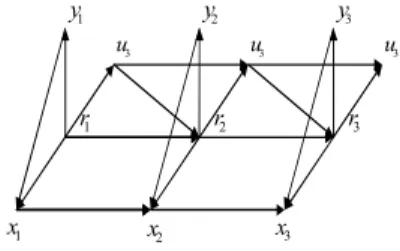
The oriented dependence graph of the model (18)-(20) is presented in Figure 2. 1 r r3 1 x x2 x3 2 r 1 y y2 y3 3 u u3 u3

Fig. 2. Oriented graph dependence of a semi-Markov switching model (18)-(20).

V. PARAMETER ESTIMATION AND EXPERIMENTS

The common point in the different models presented in the previous sections is that the distribution of the triplet

) , , ( 1 1 1 N N N Y R

X is defined in two stages: first, one defines the distribution _p(_r1N,_y1N) _{of ( , )}

1 1

N N _Y

R , and then the distribution ( ₁N ₁N, ₁N)

y r x

p is defined by the linear equation (20). When ( ₁N, ₁N)

Y

R is a Markov chain with Gaussian )

(_y1N_r1N

p , all the parameters can be estimated by “Iterative Conditional Estimation” (ICE) as described in [4]. When

) ,

(_R1N _Y1N _{is a partially Markov chain with Gaussian}

) (_y1N_r1N

p , all the parameters can still be estimated by ICE, as described in [8]. Thus we can consider “partially” unsupervised processing in both (4)-(5) (MMSHM) and (12)-(13) (HMSCLM) models: filtering and smoothing can be performed once the parameters of ( ₁N ₁N, ₁N)

y r x

p defined

with (5) – or with (13), which is identical – are known. The interest of these different models in real situations has to be tested by experiments, some of which are in progress. However, as shown by the following simple simulation study, they seem to be very powerful and promising.

Let us consider the following model N R₁ is a Markov chain; (21) X_n=F_n(R_n)X_n−₁+G_n(R_n)W_n; (22)

∏

= = N n n n N N N r y p x r y p 1 1 1 1 , ) ( ) ( , (23)

which is a very simple particular case of the model (4)-(5). We simulate data according to the classical model (1)-(3) and then they are filtered by two methods. The first one is the classical particle filtering based method explained in [1]. The second one is the exact method based on the MMSHM (21)-(23). The parameters of the hidden Markov chain

) , ( ₁N ₁N

Y

R needed in the MMSHM used are estimated with an “adaptive” ICE and the parameters in (22) are the same as the parameters in (2) used for simulation. Notice that the distribution of R₁N is known; however, to make the filtering more unsupervised in the second method we use the distribution of _RN

1 which is estimated with ICE.

The model (1)-(3) considered is given by a two-state stationary Markov chain taking its values from Ω=

{

λ₁,λ₂

}

. The parameters used to simulate realizations of the triplet

) , , ( 1 1 1 1 N N N N Y R X

T = are the following. The initial distribution of (₁N)

r

p is p₁=

(

0.5,0.5

)

, and the transitions are p

(

r₂r₁=r₂

)

=1−ρ, p

(

r₂r₁≠r₂

)

=ρ. The remaining parameters are Fn(λ1)=−0.5, Fn(λ2)=0.5, Hn(λ1)=−2, 2 ) (λ2 = n H , Gn(λ1)=0.5, Gn(λ2)=1, Jn(λ1)=1, and

2 ) (λ₂ =

n

J . We consider N=1000 for the sample size and the results for four different values of ρ are presented in Table 1, where the difference between x and the filtered _n xˆ _n is measured by x x N N n n n ˆ ) ]/ ( [ 2 1

∑

= − . One example of simulated trajectory and filtered results (last fifty points), corresponding to ρ=0.35, is presented in Figure 3.

The presented results, and others experiments results we performed, show that the semi-unsupervised (21)-(23) based method always takes upper hand over the particle filtering based one. 955 960 965 970 975 980 985 990 995 1000 -10 -5 0 5 10 (a) 955 960 965 970 975 980 985 990 995 1000 -3 -2 -1 0 1 2 3 (b) 955 960 965 970 975 980 985 990 995 1000 -3 -2 -1 0 1 2 3 (c)

Fig. 3. (a): simulated N

r1 (top),

N

x1 (dotted line), and

N

y1 (double dotted line); (b): N

x1 (dotted) and PF based

N

xˆ (double dotted) (c): 1

N

x1 (dotted) and MMSHM based

N

xˆ (double dotted). 1

ρ 0.10 0.35 0.65 0.90

PF 0.96 0.99 0.99 1.05 MMSHM 0.78 0.89 0.89 0.95

Table 1. Errors of filters based on PF and MMSHM measured by

N x x N n n n ˆ ) ]/ ( [ 2 1

∑

= − . VI. CONCLUSION

We have considered the problem of filtering and smoothing in the presence of stochastic switches. Thus there is a triplet _T1N =(_X1N,_R1N,_Y1N) _{of random chains, where X}N

1

is hidden continuous, N

R1 is hidden discrete, and N

Y1 is

observed continuous. Usually, the distribution (₁N) t p of N T₁ is given by ( ₁N, ₁N) r x p and ( ₁N ₁N, ₁N) r x y

p , which makes the computations of [ ₁n] ny X E and [ ₁N] ny X E with complexity polynomial in time unfeasible and different approximations

methods are needed. Here we exploited recent ideas according to which (1 )

N

t

p can also be defined by )

, (_r1N _y1N

p and _p(_x1N _y1N,_r1N)_{. This key point makes} filtering and smoothing computations feasible in different general models [9]-[11]. The contribution of this paper was to extend the computation of the conditional expectations

] [ 1 n ny X E and [ 1 ] N ny X

E to the computation of any conditional moments [( )m ₁n] n y X E and [( )m ₁N] n y X E , which

makes the computation of the marginal posterior distributions ( ₁n) ny x p , ( ₁N) ny x

p feasible with any desired precision. In addition, some experiments based on the very simple model proposed in [9] show the interest of the new models with respect to the classical particle filtering based methods.

As perspectives, we can mention the study extensions of the different models to general Bayesian networks [7].

REFERENCES

[1] C. Andrieu, C. M. Davy, and A. Doucet, “Efficient particle filtering for jump Markov systems. Application to time-varying autoregressions”, IEEE Trans. on Signal Processing, vol. 51, no. 7, pp. 1762-1770, 2003.

[2] O. Cappé, E. Moulines, and T. Ryden, “Inference in hidden Markov

models”, Springer, 2005.

[3] O. L. V Costa, M. D. Fragoso, and R. P. Marques, “Discrete time

Markov jump linear systems”, New York, Springer-Verlag, 2005.

[4] S. Derrode and W. Pieczynski, “Signal and image segmentation using pairwise Markov chains”, IEEE Trans. on Signal Processing, vol. 52, no. 9, pp. 2477-2489, 2004.

[5] P. Doukhan, G. Oppenheim, and M. S. Taqqu, “Long-Range Dependence”, Birkhauser, 2003.

[6] A. Doucet, N. J. Gordon, and V. Krishnamurthy, “Particle filters for state estimation of Jump Markov Linear Systems”, IEEE Trans. on

Signal Processing, vol. 49, no. 3, pp. 613-624, 2001.

[7] F. V. Jensen, Introduction to Bayesian network, Springer-Verlag, 1996.

[8] P. Lanchantin, J. Lapuyade-Lahorgue, and W. Pieczynski, “Unsupervised segmentation of triplet Markov chains hidden with long-memory noise”, Signal Processing, vol. 88, no. 5, pp. 1134-1151, 2008.

[9] W. Pieczynski, “Exact calculation of optimal filter in semi-Markov switching model”, In Proc. Fourth World Conference of the

International Association for Statistical Computing (IASC 2008),

December 5-8, Yokohama, Japan, 2008.

[10] W. Pieczynski and F. Desbouvries, “Exact Bayesian smoothing in triplet switching Markov chains”, In Proc. Complex data modelling

and computationally intensive statistical methods for estimation and prediction (S. Co 2009), September 14-16, Milan, Italy, 2009.

[11] W. Pieczynski, N. Abbassi, and M. Ben Mabrouk, “Exact filtering and smoothing of Markov switching linear system hidden with Gaussian long-memory Noise”, In Proc. XIII International

Conference Applied Stochastic Models and Data Analysis (ASMDA 2009), June 30- July 3, Vilnius, Lithuania, 2009.

[12] B. Ristic, S. Arulampalam, and N. Gordon, “Beyond the Kalman

Filter - Particle filters for tracking applications”, Artech House,

Boston, 2004.

[13] J. K. Tugnait, “Adaptive estimation and identification for discrete systems with Markov jump parameters”, IEEE Trans. on Automatic

Control, vol. AC-25, pp. 1054-1065, 1982.

[14] O. Zoeter and T. Heskes, “Deterministic approximate inference techniques for conditionally Gaussian state space models”, Statistical