HAL Id: hal-02392120
https://hal.archives-ouvertes.fr/hal-02392120
Submitted on 12 Dec 2019
HAL is a multi-disciplinary open access
archive for the deposit and dissemination of
sci-entific research documents, whether they are
pub-lished or not. The documents may come from
L’archive ouverte pluridisciplinaire HAL, est
destinée au dépôt et à la diffusion de documents
scientifiques de niveau recherche, publiés ou non,
émanant des établissements d’enseignement et de
Component trees for image sequences and streams
Caglayan Tuna, Behzad Mirmahboub, François Merciol, Sébastien Lefèvre
To cite this version:
Caglayan Tuna, Behzad Mirmahboub, François Merciol, Sébastien Lefèvre.
Component trees
for image sequences and streams. Pattern Recognition Letters, Elsevier, 2020, 129, pp.255-262.
�10.1016/j.patrec.2019.11.038�. �hal-02392120�
Component trees for image sequences and streams
Caglayan Tunaa,∗, Behzad Mirmahbouba, Franc¸ois Merciola, S´ebastien Lef`evrea
aUniv. Bretagne Sud, UMR 6074 IRISA, 56000 Vannes, France
Abstract
Morphological hierarchies now form a well-established framework for (still) image modeling and processing. How-ever, their extension to time-related data remains largely unexplored. In this paper, we address such a topic and show how to analyze image sequences with tree-based representations. To do so, we distinguish between three kinds of models, namely spatial, temporal and spatial-temporal hierarchies. For each of them, we review different strategies to build the hierarchy from an image sequence. We also propose some algorithms to update such trees when new images are appended to the series and we compared the time complexity with tree building from scratch. We illustrate our findings with the max and min-tree structures built on grayscale data provided by Satellite Image Time Series that are gathering a growing interest in Earth Observation. Besides, we provide a comparative study for different hierarchies with classification experiments.
1. Introduction
Mathematical Morphology (MM) is a well-established framework for spatial analysis of digital images since the 1960s. The two last decades have seen a significant effort devoted to morphological hierarchies, which led to e ffi-cient tools operating on the tree representations instead of the raw images (Jones, 1999). Many studies have been re-ported for mathematical morphology on image sequences (Nhimi et al., 2018; Xu and Corso, 2016; Guttler et al., 2017) but less have been reported for specifically tree rep-resentations of image sequences (Salembier et al., 1998; Alonso-Gonz´alez et al., 2014); while image sequence pro-cessing is becoming a tremendous tool to analyze spatial-temporal data in all areas of natural science. An image se-quence could be built from a continuous video acquisition or as a combination of multiple observations of the same scene acquired at different times. In this paper, we will focus on designing tree representation models for image sequences. While our findings remain generic, we will
il-∗
Corresponding author:
Email address: [email protected] (Caglayan Tuna)
lustrate them with Satellite Image Time Series (SITS) in the context of Earth Observation (EO).
One of the distinctive feature of SITS is their stream-ing nature with new acquired images appended to the se-ries. Indeed, new satellite missions such as Sentinel pro-vide images for all around the Earth every 5 days (Dr-usch et al., 2012). Updating tree representation is then an important challenge to analyze streaming data. Be-yond exploring how to build a tree from an image time series, we also focus on how to update such a tree when the time series is indeed a data stream. In the literature, this problem of trees changing over time is known as the dynamic tree problem (Sleator and Tarjan, 1983). Our im-age streaming algorithms rely on temporal based stream-ing while there are other perspectives such as spatial im-age streaming (Gigli et al., 2018). As a related work, au-thors proposed streaming graph for video segmentation in (de Souza et al., 2015).
Adding a temporal dimension to a 2D digital image offers many alternatives to build a morphological hierar-chy. The spatial and temporal dimensions may be consid-ered simultaneously or successively. The tree may contain nodes defined on the spatial, temporal, or spatial-temporal
domain. Therefore, we focus on spatial, temporal and spatial-temporal hierarchies, respectively in Sec. 3, Sec. 4 and Sec. 5. For each hierarchy, we explain how it can be built from an image sequence, relying on existing defini-tions and algorithms previously introduced on 2D images with pixels defined as scalars or multivariate data.
To the best of the authors’ knowledge, only a few stud-ies have been reported related to tree-based representa-tions exploiting the temporal dimension. Extension of the binary partition tree was considered in (Palou and Salembier, 2013), (Vilaplana et al., 2008) and (Falco et al., 2013), with some spatial and spatial-temporal hierarchies respectively. These both kinds of hierarchies have also been explored with the α-tree model in (Soille, 2008). Conversely to these previous works that focus on a parti-tioning tree and a specific hierarchy, we provide a compar-ative study of the available strategies for image sequences with component tree and extends them with streaming al-gorithms. Some illustrative experiments have been con-ducted with filtering and classification tasks on Sentinel-2 data. Another contribution of our paper is the introduction of temporal-streaming algorithms for each hierarchy.
For the sake of simplicity, we will assume in the sequel grayscale images (or time series). Nevertheless, extension of the proposed methods to multivariate data (e.g. color or multispectral images) can be achieved by relying on existing solutions for multivariate morphology (Aptoula and Lef`evre, 2007) and hierarchies (Naegel and Passat, 2009; Carlinet and G´eraud, 2015). Similarly, while we focus here on the component trees, the proposed solutions can be also easily adapted to other kinds of trees, either inclusion trees (e.g. tree of shapes) or partitioning tree (e.g. α-tree, binary partition tree, etc.).
The rest of the paper is organized as follows. Sec. 2 provides the mathematical background. We then focus on spatial, temporal and spatial-temporal hierarchies in Sec. 3, Sec. 4 and Sec. 5, respectively. For each of them, we discuss various options for constructing the hierarchy, and we explain how to update it in case of streaming data through the introduction of novel algorithms. Section 6 illustrates the experiments on a satellite image time series, before conclusion and perspectives are drawn in Sec. 7.
2. Background and notations
The structure of a tree depends on the hierarchy rule, leading to either inclusion or partitioning trees (Bosilj et al., 2018). In the former, the leaf nodes are defined as regional extrema (maxima for a max-tree), which are ex-tended and merged from leaves to root, which covers the whole image domain. In the latter, any level cut covers the whole image domain. The regions built at one level are obtained by merging the existing adjacent regions at the previous level (Souza et al., 2016). As already stated, we focus on the max and min-tree but our methodology can be applied with other models.
We will note I a grayscale image defined on the domain Ω ∈ N2 and taking values in V, i.e. I : Ω ∈ N2 → V ∈
Z, (i, j) 7→ I(i, j) = v. For the sake of conciseness, we will write x = (i, j) the coordinates of a pixel with grayscale intensity v. We assume the image being equipped with an ordering relation ≤ (the natural order among scalars).
Given a threshold λ ∈ Z, the upper threshold set is de-fined as [I ≥ λ]= {x ∈ Ω, I(x) ≥ λ}. We note the upper level set Lλ(I) = CC([I ≥ λ]) = {x ∈ Ω | CC(I(x) ≥ λ)} where CC(X) denotes the set of connected components of X. In a 2D image, a connected component is a group of adjacent pixels using 4- and 8-connectivity rules. The up-per level set Lλ(I) provides the hierarchy rule of the max-tree: two connected components (or nodes of the tree) are either disjoint or nested, and the leaves correspond to the regional gray level maxima. We write Nλa node of the tree at level λ, so Nλ = CC(Lλ(I)). A node N = (v, e) consists of pixel values v and their associated edges e. A tree T = (N, p) is then defined as the set of all nodes N and their associated edges gathered into a set of paths p. With image sequences, the coordinates combine both spatial and temporal information, noted x = (i, j) and t, respectively. Here t represents one timestamp within the entire sequence of length n, and we note Itthe
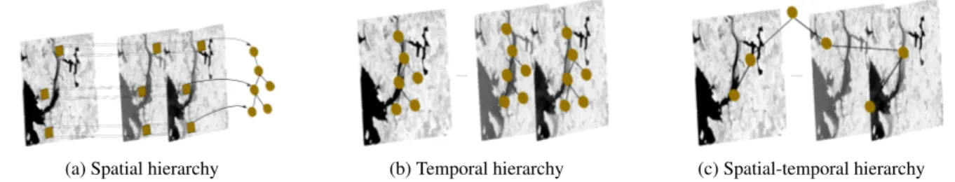
correspond-ing still image. We also write I(x, t) the value at spatial-temporal coordinates x and t, and I(x) the time series at spatial coordinates x. Figure 1 provides the different kinds of trees that are introduced in the next sections to describe an image sequence.
In this paper, we also cope with streaming situations. In such a case, an image sequence or time series is contin-uously enriched/updated with some new data coming at a (usually regular) periodicity. Instead of reconstructing
(a) Spatial hierarchy (b) Temporal hierarchy (c) Spatial-temporal hierarchy
Figure 1: Tree representation strategies: (a) a tree structure is built based on vectors of pixels in time series, (b) a tree structure is built for each image separately and these trees can be merged optionally, (c) the time series image is considered as a 3D image and a tree structure is built in three dimensions.
a new tree from scratch, a much more relevant scenario consists in updating the existing tree with the new infor-mation brought by the additional image In+1.
3. Spatial hierarchy
Despite the fact that an image sequence combines both spatial and temporal information (i.e. every data instance is made of both spatial locations and timestamp), it can still be modeled by a spatial-only hierarchy. In this case, the series of image frames ¯I= {I1, . . . , In} is first mapped
into a single, representative image ¯I (or in other words, each pixel time series I(x) leads to a single timeless value ¯I(x)). Then, a spatial hierarchy (SH) is built from this representative image. By doing so, every node of the tree has a spatial support, similarly to still images (see Sec. 2). In order to ensure compatibility with the standard max-tree algorithm, we assume the representative image to be defined on grayscales, ¯I : Ω → Z. We consider here two strategies to build the representative image: ranking or projection.
3.1. Ranking
3.1.1. Tree construction
In order to derive a single representative of an image sequence, and to use it subsequently to build a max-tree, a first approach consists in ranking all pixel time series I(x, t). Such a strategy provides a behavior similar to a standard vector ordering used in multivariate morphology, with an ordering among pixel time series. Multivariate morphology has received a lot of attention (Aptoula and Lef`evre, 2007). We recall that a binary relation that is
reflexive and transitive is called a pre-ordering (or quasi-ordering). It becomes an ordering if also anti-symmetric. Both pre-orderings and orderings could be total if the to-tality property is met, partial otherwise. Toto-tality property is required here since comparison between all pixel time series is needed to produce the representative image by means of ranking.
We thus distinguish between total orderings and total pre-orderings. The former is the most satisfactory solu-tion since it ensures a bijecsolu-tion between the set of pixel time series and their ranks. In other words, such a rank image can be modeled as a max-tree, processed with ded-icated algorithms, and the resulting (updated) rank image reprojected into an image sequence. Indeed, thanks to the total ordering of all time series, it is possible to replace every rank by the corresponding initial time series. This behavior is appealing but unfortunately the total orderings are often unbalanced in practice (Aptoula and Lef`evre, 2008). Nevertheless, we will experiment such a strategy with the most popular solution, namely the lexicographi-cal ordering that compares the first dimension (here times-tamp), and proceeds to further comparison on the second dimension only if ties appear on the first one (and so on until reaching the last dimension to assess a strict equality between vectors). Lexicographical ordering is common for color morphology such as in (Perret et al., 2012) but usage of this ordering for time series morphology is new. Relaxing the anti-symmetry constraint leads to the so-called pre-orderings. Ranking time series with a pre-ordering brings one major drawback. Due to the lack of anti-symmetry, it is possible for two different vectors (or time series) to be given the same rank. It does not pre-vent to obtain a representative image, to build a max-tree
Table 1: List of operations used in the streaming algorithms. Operation Description
create(n) creates a node “n” insert(n,v) adds value “v” to node “n”
link(n,w) creates a path between “n” and “w” nodes merge(n,w) → m merges nodes “n” and “w” into the node “m” cut(n) removes node “n”
remove(v) removes value “v” from its node neighbors(v) Connected pixels of pixel “v”
findchangedplaces Find the changed locations after new image findparent(n) Find parent node of “n”
out of it, to process the max-tree and to return a resulting representative image. Nevertheless, it will not be possible to reconstruct the image sequence from this updated rank image without arbitrary choice among time series having equal ranks. So this strategy is relevant only if the ob-jective is not filtering (or any other tasks that require re-construction). The two main categories of pre-orderings are conditional and reduced orderings. While the former considers sequentially a subset of dimensions, the latter reduces vectors to scalar values before ranking them ac-cording to their natural order. Reduced pre-orderings can be further categorized into either distance and projection-based. A popular distance-based approach orders vec-tors according to their distance from a reference vector (Celebi, 2009). In (Angulo, 2007), authors proposed sim-ilar concept for color morphology. In the context of time series, one can rely on dedicated distance metrics such as Dynamic Time Warping (DTW) (M¨uller, 2007). Since the choice of a reference time series might be a challeng-ing problem, it is possible to rely instead on the average distance to a set of reference pixels. Projection-based or-derings will deserve a specific discussion in Sec. 3.2. The construction of the representative image is done in two steps. First, all pixels in the image are ordered by applying a given vector ordering or pre-ordering on their respective time series. The pixels are then ranked, starting with rank 0 for the smallest one, and ending with rank |Ω| (in case of total ordering, lower otherwise) for the largest one. Con-struction of the max-tree is finally achieved based on the pixel ranks.
3.1.2. Streaming
The ranking approach requires the comparison of all time series from the image sequence. With the arrival of a new image, the ranks most probably need to be
calcu-Algorithm 1 Update SH Require: T (Ir), Ir0
Ensure: Updated Tree: T (I0r)
1: l= f indchangedplaces(Ir0− Ir) // changed
lo-cations
2: T (I0
r)= T (Ir) // initial tree 3: for each changed location x in l do
4: remove(Ir(x)) 5: a= I0 r(x) 6: if C(Na) < a < P(Na) then 7: insert(Na, Ir0(x)) 8: else 9: create(Na0) 10: insert(Na0, Ir0(x)) 11: findparent(Na0) 12: link(Na0, P(Na0) 13: if neighbors(a)= ∅ then 14: cut(Na) 15: link(C(Na), P(Na)) 0 0 0 0 0 5 0 1 0 0 0 3 2 5 4 0 0 0 0 0 0 5 0 1 0 0 0 3 2 3 4 0 0 0 0 0 0 5 0 1 0 0 0 3 2 6 4 0 0 2 4 5 1 3 5 0 2 3 4 1 3 5 0 2 4 6 1 3 5 Ir I0 r Ir00 T (Ir) T (I0 r) T (I00 r)
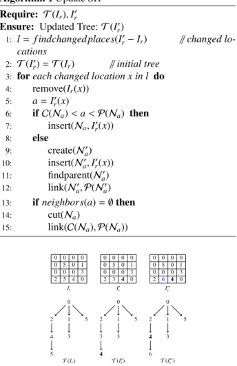
Figure 2: Streaming for spatial hierarchy
lated again. The only exception is with a conditional or-dering (including the lexicographical oror-dering) relying on the chronological order for which only pixels with equal ranks need to be compared on the new image.
Table 1 provides some operations used in all algorithms introduced in this paper. Figure 2 illustrates the simple update of a max-tree after a single pixel change. Ir
rep-resents image of ranks and it is successively updated in I0
r and Ir00. Tree nodes are represented by their level. The
blue number represent changed pixels, and the bold ones pixels that do not change in the initial image but in the tree.
We provide in Algorithm 1 the pseudo-code to update the spatial max-tree built on ranking. We note Ir(x) the
ranked pixel time series in a location x and Ir0(x) its up-dated value. P and C represent level of the parent node and child node of their content, respectively. When a new image appears, Irwill become Ir0with some changes. In
that algorithm, first, locations of the changed pixels are determined by simply calculating difference between Ir
and Ir0 and locations are stored in l. Then new pixels a
are placed on a tree according to their intensity value and connectivity. If a changed value is between parent node level and child node level, it remains to be in the same node. Otherwise its location will change and a new node should be created for the new value. This algorithm is repeated for each changed location. More precisely, the time complexity increases if the amount of changed value increases. Lines 13 and 14 remove the node if there is no connectivity between a changed location and its neigh-bors. After removal, parent and child nodes are connected to each other.
3.2. Projection
3.2.1. Tree construction
A specific reduced pre-ordering relies on projections, i.e. mapping the vectors into scalar values on which the comparison is performed such as in (Velasco-Forero and Angulo, 2012) for color images. While this approach still corresponds to the application of a vector ordering, it of-fers some specific advantages that calls for additional dis-cussion. First, applying the vector ordering is straightfor-ward since it only consists in relying on the natural order-ing between scalars. Conversely to the previous strategy, there is no need to rank pixels to build the representative image.
The projection relies on a function f : Nn → N, x 7→ f(I(x, 1), . . . , I(x, n)). We still write ¯I(x) the output scalar value for this location. Depending on the application con-text, a wide range of functions are available e.g. mean, median, standard deviation, range, etc. In the most prob-able case of a non-injective function, this strategy also faces the difficulty of reconstructing the image sequence from the processed max-tree. Here, the projection func-tion was defined as Nn → N, but max-tree algorithms are
not restricted to natural numbers and can be applied also on real-valued images.
3.2.2. Streaming
The streaming rules are the same as in Algorithm 1. To ease updating, one might prefer functions that do not require a full recomputation (e.g. mean or standard de-viation if the sum and squared sum are stored). Another advantage is the fact that the update can be done in paral-lel, similarly to the initial projection.
4. Temporal hierarchy
Alternatively, the temporal hierarchy (TH) allows us to process each image and to build the tree representation for each of them separately. We first explain the tree con-struction process and then how to update the tree during the streaming step.
4.1. Tree construction
After building a tree for each image, we have two op-tions to process them. We can process each tree inde-pendently (eg. extracting features) and stack the results together that is called marginal approach (Aptoula and Lef`evre, 2007). Every image Itof the series might have its
own tree T (It). It is a straightforward technique to build
a tree (similarly to the standard still image case), leading to T (I1), . . . , T (In). This approach provides marginally
processing such as in (Dalla Mura et al., 2010) and tree structure comparison (Bracci et al., 2017). The second option is to merge initial trees together and process the final tree. The critical merging step is a special case of streaming that we will explain in next subsection. 4.2. Streaming
In the marginal case, streaming is straightforward and consists in sequentially adding a new tree to the set of initial trees. On the other hand, merging trees is not a straightforward process due to the memory and compu-tational costs brought by the spatial-temporal connectiv-ity. Existing methods to build the max-tree usually pro-ceed by merging trees corresponding to some small parts in the image separately (G¨otz et al., 2018), while tree of shapes (Carlinet and G´eraud, 2015) or α-tree (Havel et al., 2016) have also led to parallel algorithms with merging and (Moschini et al., 2018) deals with extreme dynamic range data by merging sub-trees of sub-images.
Algorithm 2 Update TH Require: T (I1), T (I2)
Ensure: Tm
1: R(T (m) = merge(R(T (I1)), R(T (I2))) // initial
root
2: for ∀λ ∈ λ1∩λ2do // for all levels 3: for ∀N1∈ T (I 1) do 4: for ∀N2∈ T (I 2) do 5: if N1∩ N2= x and I 1(x)= I2(x) then 6: a= I2(x) 7: Na= merge(Na1, Na2)|Na∈ Tm 8: else if then 9: N1, N2∈ Tm
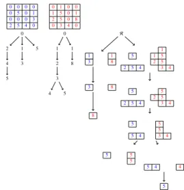
Figure 3 illustrates the merging of two max-trees by in-creasing the connectivity from 4 to 6 neighbors. The two images on the left are shown with their respective trees. The merged tree is given on the right. For the sake of conciseness, we have omitted intensity values from the tree representation of the two initial images. Algorithm 2 provides the pseudo-code for merging max-trees. R rep-resents the root of the tree and Tmis the merged tree.
Be-sides, N1and N2represent the nodes for first and second
image respectively. Output of Algorithm 2 is a multidi-mensional tree i.e. a space-time tree which will be ex-plained in the next section. More precisely, connectivity of T (I1), T (I2) is 4 but connectivity of Tm is 6. Since
Tmstill includes pixels from previous images, streaming
preserves past information. In that algorithm, first, the initial root is created. Thus, two trees transform to one tree. Then, connectivity between nodes is investigated from root to leaves. If a node has no connectivity to other tree nodes, it is kept in the tree without merging.
5. Spatial-temporal hierarchy
The last strategy is the spatial-temporal hierarchy (STH). In this approach, one tree is built for the whole image time series and processing this tree gives a multidi-mensional image set.
5.1. Tree construction
The image sequence can be seen as a spatial-temporal cube, where each date corresponds to one layer, the two
0 0 0 0 0 5 0 1 0 0 0 3 2 5 4 0 0 1 0 0 1 5 0 1 2 5 0 8 0 3 4 0 R 1 3 1 8 5 2 5 4 1 1 5 2 5 3 4 5 2 5 4 5 2 5 3 4 3 8 5 5 4 5 5 3 4 8 5 4 4 5 5 5 5 0 2 4 5 1 3 5 0 1 2 3 4 5 1 8
Figure 3: Tree for each date and streaming by merging. Two images and their max trees are in the left and merged tree is in the right
other dimensions being the spatial ones. From this cube it is possible to build a spatial-temporal tree, i.e. a sin-gle tree that includes all information from the whole time series (T (I1, . . . , In)). However, building such a complex
tree given a long time series is particularly challenging due to scalability issues. While 3D data has received less attention than 2D, still a few works have been proposed to compute trees on such data, e.g. (Westenberg et al., 2007) and (Wilkinson et al., 2008) for 3D computed tomogra-phy (CT) images, or (Alonso-Gonz´alez et al., 2014) for 3D SAR time series.
The major difference with a still image is the change in terms of connectivity due to the extension to a third dimension. Conversely to a 2D image that comes with 4- and 8-adjacency, space-time tree offers us 6-, 18- and 26-adjacency. In the specific context of a spatial-temporal cube, one might prefer anisotropic behavior, thus leading for instance to a 10-neighborhood (made from the union of the spatial 8- and temporal 2-adjacency).
5.2. Streaming
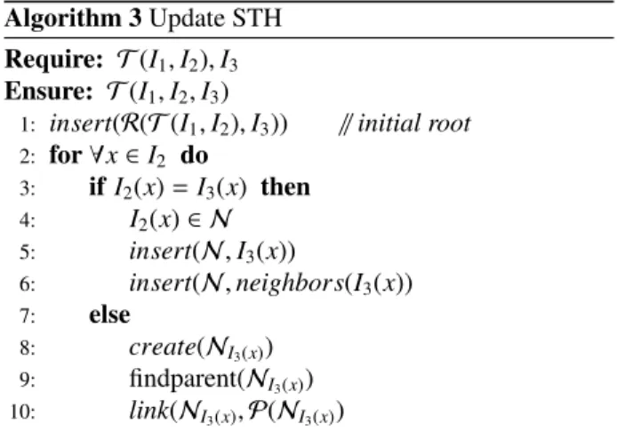
The streaming strategy is similar to the one used for merging trees but here we use only a new image instead of a new tree. Figure 4 shows an updated space-time max-tree after the third image. Different colors are used for different images in order to avoid confusion in the nodes.
0 0 0 0 0 5 0 1 0 0 0 3 2 5 4 0 0 1 0 0 1 5 0 1 2 5 0 8 0 3 4 0 1 0 0 0 0 5 5 1 2 0 0 3 0 4 4 1 R 1 3 1 8 5 2 5 4 1 1 5 2 5 3 4 5 2 5 4 5 2 5 3 4 3 8 5 5 4 5 5 3 4 8 5 4 4 5 5 5 5 R 1 5 1 3 2 5 4 1 1 5 1 5 5 8 3 4 5 5 1 2 3 4 4 1 5 2 5 4 5 2 5 3 4 5 5 2 4 4 3 5 3 5 5 4 5 5 3 4 5 5 4 4 5 5 5 5 5 5 4 4 4 4 8 5
Figure 4: Cube tree and streaming (Two images and their space-time tree in the left, new image and updated space time-tree in the right)
Two images and their space-time trees are shown on the left, the new image and the updated space-time tree being given on the right. Algorithm 3 provides the pseudo-code for updating a space-time max-tree. Here, connectivity rule remains to be 6 but nodes are extended to include new image information. First, all new image is inserted to root. Then new image pixels are placed on a tree according to their location and gray values. Similarly to merging trees, streaming a space-time tree preserves information from previous images, which is important for time-related EO applications.
6. Experiments
Tree representation can be used for several applications such as filtering, classification, segmentation, change de-tection, or object detection (Bosilj et al., 2018). In this paper, we consider two use cases related to satellite im-agery. First, the classification of Satellite Image Time Se-ries (SITS) that allows quantitative assessment. Second, image filtering for which visual analysis is provided. We used an open source node-oriented max-tree toolbox in our experiments (Souza et al., 2015) and we report the re-sults in this section. The codes for our classification and
Algorithm 3 Update STH Require: T (I1, I2), I3
Ensure: T (I1, I2, I3)
1: insert(R(T (I1, I2), I3)) // initial root 2: for ∀x ∈ I2 do 3: if I2(x)= I3(x) then 4: I2(x) ∈ N 5: insert(N, I3(x)) 6: insert(N, neighbors(I3(x)) 7: else 8: create(NI3(x)) 9: findparent(NI3(x)) 10: link(NI3(x), P(NI3(x))
filtering experiments are also publicly available1.
6.1. Classification
We apply classification algorithms to SITS to evaluate the relevance of the proposed tree representation strate-gies. We used a sample SITS made of small extracts (1000 px ×1000 px) from 17 Sentinel-2 images (at 10m/px res-olution) which were acquired in 2016 around Dordogne, France. We selected only cloud-free images for our ap-plication. We used level 2A products provided by the THEIA land data center. We extract labelled data from the agricultural Land Parcel Information System known as Registre Parcellaire Graphique (RPG). The studied area includes 5 land cover classes: urban (yellow), crop (red), water (blue), forest (green) and moor (pink). Since our focus is on the image time series, we simplify each mul-tispectral image into a grayscale one by computing the Normalized Difference Vegetation Index (NDVI) in each pixel. In order to achieve classification, we inspire from the recent work on feature profiles (Pham et al., 2017). We calculated node attributes such as area, mean gray value, height and volume, then we used these attributes as a fea-ture for each location.
Both min and max-tree are used to obtain feature ages. These images are then stacked with the original im-age time series and the whole set is used for classification. In our experiments, we split vertically the image into two
1https://github.com/caglayantuna/
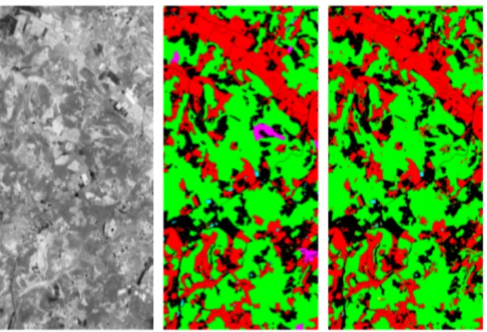
Figure 5: SITS Classification (from left to right): Sentinel-2 extract (date 1), reference map and sample result.
equal parts to obtain independent train and test sets.. The first part of the image was used for training and valida-tion, following a 5-fold cross validation procedure. As a classifier, we used the Random Forest method (Breiman, 2001). We optimized the number of trees and maximum depth among the variables {100, 200, 300} and {80, 90, 100} during this process. Then, we used the best param-eters and evaluate the classification performance with the testing set. As the baseline, we considered original SITS pixels described by NDVI values as input features and classified the image. We obtained an overall accuracy of 93.63. Figure 5 provides a qualitative result from the test area with the first image of the multitemporal Sentinel-2 image and its associated reference map. Each color rep-resent a specific land cover class (and black for ignored pixels). Table 2 reports the classification results obtained with each tree representation strategy and different spatial features. Results show that the spatial features offer an efficient way to increase the classification accuracy with TH and STH strategy comparing to the baseline, i.e. with-out using spatial features. Table 3 provides an additional evaluation measure, namely f1score for each class.
According to these results, SH is not adequate to clas-sify SITS, but on the other hand, it can be used for other applications. For example, in our previous work (Tuna et al., 2019), we proposed a SH approach for change de-tection, through filtering tree with a projected SITS. 1636, 133374, 2010, 226231 and 5354
Table 2: Comparison of overall classification accuracy
Methods Spatial features
Area Mean gray value Height Volume
SH-Lex. 56.31 57.52 57.14 57.64
SH-DTW 78.52 75.08 77.15 78.26
SH-Mean 60.97 70.38 61.25 75.25
TH-Marginal 94.52 94.44 94.45 94.26
STH-Space-time 94.20 94.11 94.05 94.14
Table 3: Number of samples for training and testing part and F1score
for each class
Urban Crops Water Forest Moor
Nb. of samples 1381-1636 105214-133374 1754-2010 266649-226231 1901-5354 Without Profile 0.51 0.93 0.59 0.95 0.002 SH-Lex. 0.009 0.18 0.004 0.71 0.001 SH-DTW 0.17 0.68 0.009 0.83 0.003 SH-Mean 0.14 0.64 0.005 0.82 0.003 TH-Marginal 0.54 0.94 0.55 0.96 0.003 STH-Space-time 0.53 0.94 0.57 0.95 0.003 6.2. Filtering
In order to further illustrate the potential of tree repre-sentations for SITS, we provide a filtering result for one of the image in our set. Filtering relies on pruning the tree according to some criteria such as attribute thresh-olds. First, attributes are calculated for each node sepa-rately. Then, some nodes are removed if their attributes are smaller than a user-defined threshold (Jones, 1999). Pixel values in these nodes are changed according to their connectivity. Last, the pruned tree is reconstructed and the filtered image is subsequently obtained.
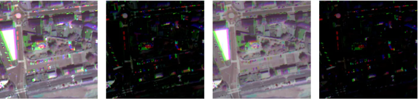
Figure 6 is the outcome of a filtering experiment con-ducted with three panchromatic Pleiades images acquired over the same scene at different date, as provided by Kalideos2. As a baseline, we built a tree for of each date
and applied a filtering without considering the temporal information. We also stacked these images and built a space-time max-tree corresponding to the STH strategy. We used here the area attribute (i.e. amount of pixels in a node). We use a unique threshold (1000) to allow fair comparison. As mentioned in Sec. 2, max-tree leaves include regional extrema of the image. Therefore, max-tree filtering allows manipulating bright objects in the im-age. To emphasize the filtered objects, we show in Fig. 6 the difference between original and filtered images. We
can see that cars which are at different places for different dates are caught by the filtering. However, filtering with a single frame cannot be used to filter out only cars since it removes other objects such as the building located at the bottom left of the scene. Let us recall that this exam-ple is provided only for the sake of illustration and proper detection of dynamic objects is left for future work. 6.3. Streaming time complexity
We applied our streaming algorithms to synthetic im-ages which are shown in Fig. 2, Fig. 3 and Fig. 4. We compared time complexity of the tree building strategies with streaming and without streaming in Tab. 4. Without streaming indicates that a new tree is built from scratch when a new image appears. The complexity of Algo-rithm 1 is O(hc) where c is the amount of changed pix-els and h is the used tree levpix-els for this algorithm. This depth h value is 1 ≤ h ≤ 2bit− 1 where bit is 8 or 16
depending on the source of the image. Algorithm 2 is O(hk) where k is the amount of nodes. According to (Car-linet and G´eraud, 2014), tree building for large integers requires at least a complexity of O(nplog np) where npis
the amount of pixels of one image. Since satellite images are very large, the amount of pixels is usually huge, there-fore the amount of tree nodes is lower than the amount of pixels in the image. Although theoretical complexities for SH, TH and STH are all O(nplog np), the actual
com-putational time will be different due to various amounts of pixels/images. For example, with 3 real Sentinel-2 im-ages (10980 px × 10980 px), computation times for tree building are 75s, 133s and 211s and required memories are 3083MB, 5384MB and 7034MB for SH, TH and STH strategy respectively. The space-time streaming complex-ity requires only one image with nppixels while without
streaming requires n times amount of pixels where n is the amount of images in a set. Besides, the complexity has an extra hnncaused by the new node creation part.
Table 4: Time complexity comparison (np:Number of pixels, c:changed
pixels, h: search on the tree, k: amount of nodes, nn: amount of new
nodes )
Method Streaming Without streaming
SH O(hc) O(nplog np)
TH O(hk) O(nplog np)
STH O(np+ hnn) O(nplog np)
The complexity of the algorithms is further analyzed in Table 4 where we assess the effect of the streaming strategy. The SH streaming depends on the number of changed pixels. The proposed SH streaming algorithm is more efficient than without streaming when the number of changed pixels satisfies the following relation:
c<nplog np
h . (1)
The merging time depends on the amount of nodes in the tree levels. In the TH streaming complexity, better efficiency is ensured if k denoting the amount of nodes satisfies
k<nplog np
h (2)
Finally, the STH streaming algorithm includes a pro-cess of creating new nodes. In order the streaming to be relevant, the upper bound of the number of new created nodes should follow
nn<
nplog np− np
h (3)
7. Conclusion
While morphological hierarchies have been largely ex-plored in the literature (both from a theoretical and ap-plication point of view), their extension to time series re-mains barely addressed. In this paper, we have discussed how to build such hierarchies, considering specifically the max-tree model on gray-scale data. More precisely, we have distinguished between spatial, temporal and spatial-temporal hierarchies, that all can be built using various strategies. Here, we compared tree representation strate-gies for classification purposes. We also investigated the case of streaming, where new images or frames are ap-pended to the series, thus needing to update the under-lying tree structure in a scalable manner. We proposed streaming algorithms for all building strategies. We be-lieve that the proposed approaches will call for further studies in the field.
Let us note that all our tree models were designed to deal with temporal information and are sensitive to the or-der of images. Nevertheless, let us point two cases where
Figure 6: SITS Filtering (from left to right): composite of original series and its difference with its respective spatial-only filtering, STH filtering and its difference with the original image. Each triplet of dates is represented by a color image (one channel per date).
shuffling of images will have no effect on the result: 1) with the SH strategy, it directly depends on the proper-ties of the projection function (e.g. using the average or standard deviation is unaffected to shuffle, while using a projection based on DTW is). 2) with the TH strategy in the marginal case, it directly depends on the actual pro-cessing that is considered afterwards.
Future work will include the extension to other tree models such as tree of shapes, α or ω trees, etc. Besides, assessing the relevance of such models with time series data will be of high interest in the EO context. Generic streaming algorithms will be necessary to handle large scale EO data. Besides, extending tree representations with spectral information is worth being studied given the multispectral nature of EO time series.
Acknowledgments
This work was supported by Centre National d’ ´Etudes Spatiales (CNES) and Collecte Localisation Satellites (CLS).
References
Alonso-Gonz´alez, A., L´opez-Mart´ınez, C., Salembier, P., 2014. PolSAR time series processing with binary par-tition trees. IEEE Trans. Geosci. Remote Sens. 52, 3553–3567.
Angulo, J., 2007. Morphological colour operators in to-tally ordered lattices based on distances: Application to image filtering, enhancement and analysis. Computer vision and image understanding 107, 56–73.
Aptoula, E., Lef`evre, S., 2007. A comparative study on multivariate mathematical morphology. Pattern Recog-nition 40, 2914–2929.
Aptoula, E., Lef`evre, S., 2008. On lexicographical order-ing in multivariate mathematical morphology. Pattern Recognition Letters 29, 109–118.
Bosilj, P., Kijak, E., Lef`evre, S., 2018. Partition and inclu-sion hierarchies of images: A comprehensive survey. Journal of Imaging 4, 33.
Bracci, F., Hillenbrand, U., Marton, Z.C., Wilkinson, M.H., 2017. On the use of the tree structure of depth levels for comparing 3d object views, in: Int. Conf. on Computer Analysis of Images and Patterns, pp. 251– 263.
Breiman, L., 2001. Random forests. Machine learning 45, 5–32.
Carlinet, E., G´eraud, T., 2014. A comparative review of component tree computation algorithms. IEEE Trans. Image Process. 23, 3885–3895.
Carlinet, E., G´eraud, T., 2015. Mtos: A tree of shapes for multivariate images. IEEE Trans. Image Process. 24, 5330–5342.
Celebi, M.E., 2009. Distance measures for reduced ordering-based vector filters. IET image processing 3, 249–260.
Dalla Mura, M., Atli Benediktsson, J., Waske, B., Bruz-zone, L., 2010. Extended profiles with morphological
attribute filters for the analysis of hyperspectral data. International Journal of Remote Sensing 31, 5975– 5991.
Drusch, M., Del Bello, U., Carlier, S., Colin, O., Fernan-dez, V., Gascon, F., Hoersch, B., Isola, C., Laberinti, P., Martimort, P., et al., 2012. Sentinel-2: Esa’s optical high-resolution mission for gmes operational services. Remote sensing of Environment 120, 25–36.
Falco, N., Dalla Mura, M., Bovolo, F., Benediktsson, J.A., Bruzzone, L., 2013. Change detection in vhr images based on morphological attribute profiles. Geoscience and Remote Sensing Letters 10, 636–640.
Gigli, L., Velasco-Forero, S., Marcotegui, B., 2018. On minimum spanning tree streaming for image analysis, in: 25th ICIP, pp. 3229–3233.
G¨otz, M., Cavallaro, G., G´eraud, T., Book, M., Riedel, M., 2018. Parallel computation of component trees on distributed memory machines. Transactions on Parallel and Distributed Systems 29, 2582–2598.
Guttler, F., Ienco, D., Nin, J., Teisseire, M., Poncelet, P., 2017. A graph-based approach to detect spatiotempo-ral dynamics in satellite image time series. Journal of photogrammetry and remote sensing 130, 92–107. Havel, J., Merciol, F., Lef`evre, S., 2016. Efficient tree
construction for multiscale image representation and processing. J. Real Time Image Pr. , 1–18.
Jones, R., 1999. Connected filtering and segmentation using component trees. Computer Vision and Image Understanding 75, 215–228.
Moschini, U., Meijster, A., Wilkinson, M.H., 2018. A hybrid shared-memory parallel max-tree algorithm for extreme dynamic-range images. IEEE Trans. Pattern Anal. Mach. Intell. 40, 513–526.
M¨uller, M., 2007. Dynamic time warping. Information retrieval for music and motion , 69–84.
Naegel, B., Passat, N., 2009. Component-trees and multi-value images: A comparative study, in: International Symposium on Mathematical Morphology and Its Ap-plications to Signal and Image Processing, pp. 261– 271.
Nhimi, F.T.L., Patroc´ınio Jr, Z., Perret, B., Cousty, J., Guimar˜aes, S.J.F., 2018. Evaluation of morphologi-cal hierarchies for supervised video segmentation, in: ACM Symp. on Applied Computing, pp. 252–259. Palou, G., Salembier, P., 2013. Hierarchical video
repre-sentation with trajectory binary partition tree, in: Pro-ceedings of the Conference on Computer Vision and Pattern Recognition, pp. 2099–2106.
Perret, B., Lef`evre, S., Collet, C., Slezak, ´E., 2012. Hyperconnections and hierarchical representations for grayscale and multiband image processing. IEEE Trans. Image Process. 21, 14–27.
Pham, M.T., Aptoula, E., Lef`evre, S., 2017. Feature pro-files from attribute filtering for classification of remote sensing images. Journal of Selected Topics in Applied Earth Observations and Remote Sensing 11, 249–256. Salembier, P., Oliveras, A., Garrido, L., 1998.
Antiexten-sive connected operators for image and sequence pro-cessing. IEEE Trans. Image Process. 7, 555–570. Sleator, D.D., Tarjan, R.E., 1983. A data structure for
dy-namic trees. Journal of computer and system sciences 26, 362–391.
Soille, P., 2008. Constrained connectivity for hierarchi-cal image partitioning and simplification. IEEE Trans. Pattern Anal. Mach. Intell. 30, 1132–1145.
de Souza, K.J., Ara´ujo, A.d.A., Guimar˜aes, S.J., do Pa-troc´ınio, Z.K., Cord, M., 2015. Streaming graph-based hierarchical video segmentation by a simple label prop-agation, in: 28th SIBGRAPI Conference on Graphics, Patterns and Images, pp. 119–125.
Souza, R., Rittner, L., Lotufo, R., Machado, R., 2015. An array-based node-oriented max-tree representation, in: ICIP, pp. 3620–3624.
Souza, R., Tavares, L., Rittner, L., Lotufo, R., 2016. An overview of max-tree principles, algorithms and appli-cations, in: 29th SIBGRAPI Conference on Graphics, Patterns and Images Tutorials, pp. 15–23.
Tuna, C., Merciol, F., Lef`evre, S., 2019. Monitoring ur-ban growth with spatial filtering of satellite image time series, in: JURSE, pp. 1–4.
Velasco-Forero, S., Angulo, J., 2012. Random projection depth for multivariate mathematical morphology. IEEE J. Sel. Topics Signal Process. 6, 753–763.
Vilaplana, V., Marques, F., Salembier, P., 2008. Binary partition trees for object detection. IEEE Trans. Image Process. 17, 2201–2216.
Westenberg, M.A., Roerdink, J., Wilkinson, M.H., 2007. Volumetric attribute filtering and interactive visualiza-tion using the max-tree representavisualiza-tion. IEEE Trans. Im-age Process. 16, 2943–2952.
Wilkinson, M., Gao, H., Hesselink, W.H., Jonker, J., Mei-jster, A., 2008. Concurrent computation of attribute fil-ters on shared memory parallel machines. IEEE Trans. Pattern Anal. Mach. Intell. 30, 1800–1813.
Xu, C., Corso, J.J., 2016. Libsvx: A supervoxel library and benchmark for early video processing. Interna-tional Journal of Computer Vision 119, 272–290.