HAL Id: hal-01712148
https://hal.archives-ouvertes.fr/hal-01712148
Submitted on 8 Nov 2018
HAL is a multi-disciplinary open access
archive for the deposit and dissemination of
sci-entific research documents, whether they are
pub-lished or not. The documents may come from
teaching and research institutions in France or
abroad, or from public or private research centers.
L’archive ouverte pluridisciplinaire HAL, est
destinée au dépôt et à la diffusion de documents
scientifiques de niveau recherche, publiés ou non,
émanant des établissements d’enseignement et de
recherche français ou étrangers, des laboratoires
publics ou privés.
Analysis of Radiation Modeling for Turbulent
Combustion: Development of a Methodology to Couple
Turbulent Combustion and Radiative Heat Transfer in
LES
Damien Poitou, Mouna El-Hafi, Benedicte Cuenot
To cite this version:
Damien Poitou, Mouna El-Hafi, Benedicte Cuenot. Analysis of Radiation Modeling for Turbulent
Combustion: Development of a Methodology to Couple Turbulent Combustion and Radiative Heat
Transfer in LES. Journal of Heat Transfer, American Society of Mechanical Engineers, 2011, 133 (6),
�10.1115/1.4003552�. �hal-01712148�
Analysis of the interaction between turbulent combustion and thermal
radiation using unsteady coupled LES/DOM simulations
Poitou Damien
a,⇑, Amaya Jorge
a, El Hafi Mouna
b, Cuénot Bénédicte
aaCERFACS, 42, Avenue Gaspard Coriolis, 31057 Toulouse Cedex 01, France bCentre RAPSODEE, École des Mines d’Albi, Campus Jarlard, 81013 Albi, France
Keywords:
Large eddy simulation Radiative transfer Spectral models
Discrete Ordinate Method (DOM) Coupling
Turbulence Radiation Interaction (TRI)
a b s t r a c t
Radiation exchanges must be taken into account to improve the prediction of heat fluxes in turbulent combustion. The strong interaction with turbulence and its role on the formation of polluting species require the study of unsteady coupled calculations using Large Eddy Simulations (LESs) of the turbulent combustion process. Radiation is solved using the Discrete Ordinate Method (DOM) and a global spectral model. A detailed study of the coupling between radiative heat transfer and LES simulation involving a real laboratory flame configuration is presented. First the impact of radiation on the flame structure is discussed: when radiation is taken into account, temperature levels increase in the fresh gas and decrease in the burnt gas, with variations ranging from 100 K to 150 K thus impacting the density of the gas. Cou-pling DOM and LES allows to analyze radiation effects on flame stability: temperature fluctuations are increased, and a wavelet frequency analysis shows changes in the flow characteristic frequencies. The second part of the study focuses on the Turbulence Radiation Interaction (TRI) using the instantaneous radiative fields on the whole computational domain. TRI correlations are calculated and are discussed along four levels of approximation. The LES study shows that all the TRI correlations are significant and must be taken into account. These correlations are also useful to calculate the TRI correlations in the Reynolds Averaged Navier–Stokes (RANS) approach.
1. Introduction
Besides combustion efficiency, the design of industrial combus-tion chambers and furnaces is strongly dictated by thermal con-straints. The solid parts of a combustor are made of materials that do not support a direct contact with the high temperature burnt gases. As a consequence, chamber walls must be cooled down, using complex cooling techniques that are expensive to design, develop and operate. The inclusion of such systems modifies the tempera-ture distribution inside the chamber and hence the turbulent combustion. The thermal behavior of a combustion chamber is also critical for the downstream elements (turbines): thermal con-straints of the materials impose strict limits on the temperature levels and fluctuations in the incoming flow exiting from the combustion chamber. Finally, thermal behavior also has an impact on the production of pollutants such as CO, NOxand soot and may modify the interaction of impinging fuel droplets with the walls.
The mean temperature level in a combustion chamber is well estimated, at first order, by a simple enthalpy balance between fresh reactants and hot products. If NOxand soot are not produced, neglecting radiation and wall temperature variations still leads to
relatively accurate mean temperature levels but is responsible for errors on temperature fluctuations. The inclusion of pollutants emission re-enforces this error and introduces a deviation of the mean temperature. Such error levels are outside the tolerance range for combustor design, and it is therefore necessary to include radiation in combustion studies for the optimization of combustion chambers.
In this process, numerical simulation plays an increasingly important role. In comparison with experimental setups, numeri-cal simulation shows the advantage of being cheaper and more flexible. Its main drawback is its use of models to represent limited accuracy of the numeric complex physics. Important progress how-ever has been made in the last years, in particular with the devel-opment of the Large Eddy Simulation (LES) approach and the sustained increase of computational power. Today LES is routinely applied to industrial burners and gives accurate and reliable solu-tions, as demonstrated in the recent literature [1–3]. Computa-tional power has also been used in recent time to calculate radiation in complex geometries[4].
Radiation is a complex, non-local phenomenon in which energy is simultaneously emitted and absorbed by the gases. To correctly capture the effect of radiation, both emission and absorption must be included and coupled with combustion. This is the aim of the present work, where unsteady combustion–radiation simulations ⇑ Corresponding author.
of a laboratory burner have been performed. The main objectives of this work consist in the validation of the coupling methodology, the quantification and analysis of the interaction between the in-volved phenomena and the evaluation of the impact of radiation on the thermal behavior of the burner. To perform such coupled simulations, high-performance computing techniques must be used, as well as a reliable coupling methodology, which are an important challenge: a demonstration of the feasibility and the importance of such simulations is a main objective of this paper.
The unsteady coupling between radiation and turbulent com-bustion in LES allows studying the so-called Turbulence Radiation Interaction (TRI). This is a rich research area, which has been stud-ied experimentally, theoretically and numerically by both radia-tion and combusradia-tion communities [5–7]. Numerous works were done in the RANS context. More recently, TRI was studied with DNS[8]in an a priori way[9], in which turbulence is fully resolved and no model is used. This kind of study has however some limita-tions: small Reynolds number, simple geometry, periodic boundary conditions, etc. In the present work, an analysis is done a posteriori
[9]using LES to simulate a real burner configuration. The coupling between radiation and combustion is analyzed following the TRI formalism first proposed in RANS and DNS contexts, but uses un-steady resolved fluctuations as provided by the LES.
The present document is organized in four main parts: Section2
presents the basic aspects of the computational methods for un-steady turbulent combustion and radiative heat transfer and shows a description of the unsteady coupling methodology. In Section3, the configuration and the simulation set up is presented. Results are analyzed in Sections4–6, first by comparing the simulation uncoupled and coupled with radiation, then by a detailed descrip-tion of the interacdescrip-tion between turbulence and radiadescrip-tion. Finally, in Section 7, a summary of the main findings of this study is presented.
2. Modeling of coupled LES and radiative calculation 2.1. LES equations
The conservation equations of the fluid can be written in a ma-trix form:
@w
@t þ
r
" F ¼ s ð1Þwhere w = (
q
u,q
v,q
w,q
E,q
Yk)Tis the conservative variable vector that is solved at each location x and time t, withq
the mixture den-sity, u,v
, w the components of the velocity vector v, E the energy density and Ykthe mass fraction of the species k (16 k 6 Nspecies). The flux tensor F can be decomposed in an inviscid (noted I) and a viscous component (noted V):FI¼
v
:q
v
Tþ P ðq
E þ PÞv
q
kYkv
2 6 6 4 3 7 7 51 ð2Þ and FV¼ &s
&v
T"s
þ q Jk 2 6 4 3 7 5 ð3Þusing the hydrodynamic pressure P defined by the equation of state of perfect gas, q the heat flux and Jkthe diffusive flux of species k. The stress tensor for a Newtonian fluid
s
= [s
ij] is:s
ij¼ 2l
Sij&13dijSll ! " where Sij¼12 @uj @xiþ @ui @xj ! " ð4ÞFor a reacting flow including radiation, the source term s is written:
s ¼ ð0; 0; 0; _
x
Tþ Sr; _x
kÞT ð5Þwhere _
x
T is the chemical heat release, Sris the thermal radiative heat source and _x
kis the reaction rate for species k.A Favre filtering (defined in Eq.(6)) is used to derive the filtered balance equations for LES (Eq.(7)), which are obtained from equa-tions (Eq. (1)), assuming a commutation between the filter and derivative operator[10]:
e
/ ¼
q
q
!/ ð6Þ@ !w
@t þ
r
" F ¼ !s ð7ÞThe filtered flux tensor F contains a resolved part, expressed by Eqs.
(2) and (3)using filtered variables, and an unresolved part which is modeled in the form of a subgrid flux tensor Ft:
Ft ¼ &
s
t qt Jt k 2 6 4 3 7 5 ð8Þ wheres
t ij¼ &!q
#ugiuj& euiuej$ ð9Þ qt i¼ !q
guiE & euieE % & ð10Þ Jt i;k¼ !q
ugiYk& euifYk % & ð11ÞNote that the subgrid Reynolds stress tensor
s
t, the subgrid turbu-lent heat flux qt and the subgrid turbulent species flux Jtk model the unresolved convective transport only. Unresolved diffusive transport is neglected.
Nomenclature
CFL Courant–Friedrichs–Lewy criterion DMFS Diamond Mean Flux Scheme DOM Discrete Ordinate Method DNS Direct Numerical Simulation FS-SNBcK Full Spectrum SNBcK FSK Full Spectrum
j
(i.e. FS-SNBcK) FSCK Full Spectrum Correlatedj
FVM Finite Volume Method HR Heat Release
LES Large Eddy Simulation
NSCBC Navier–Stokes Characteristic Boundary Conditions OTFA Optically Thin Fluctuations Approximation PCS Parallel Coupling Strategy
PSD Power Spectral Density
RANS Reynolds Averaged Numerical Simulation RTE Radiative Transfer Equation
SNB Statistical Narrow Band SNBcK SNB with correlated
j
model TRI Turbulence Radiation Interaction WSGG Weighted Sum of Gray GasesMomentum, energy and species conservation equations are solved using realistic thermochemistry, i.e. real values for all ther-modynamic properties taken from reference databases for each chemical species. The subgrid model describing the turbulent stress tensor (Eq.(9)) is based on the turbulent viscosity concept using the WALE model [12]. Turbulent fluxes for thermal and species diffusion (Eqs. (11) and (10)) are modeled by classical gradient laws with turbulent Schmidt and Prandtl numbers. Characteristic boundary conditions NSCBC [13] are used for all inlets and for the outlet allowing the evacuation of acoustic energy from the domain.
The numerical calculation was performed with the unstruc-tured compressible Navier–Stokes solver AVBP,1using a 3rd order
in space and time Taylor–Galerkin scheme (TTGC[14]). 2.2. Turbulent combustion modeling
The turbulent flame front is described using the dynamic Thick-ened Flame Model (TFLES). In such a model, the reaction front is artificially thickened in order to solve stiff gradients on the grid without altering global flame characteristics. This model is detailed in[15]and has been extensively used and validated in numerous configurations[1,3,2]. Subgrid wrinkling is modeled using an effi-ciency function[15]. In the present configuration, the maximum thickening factor is Fmax= 20. A priori tests based on Direct Numer-ical Simulations[15]and a posteriori evaluation of the TFLES model on complex configurations have shown that the thickening factor should not be too large to stay in the limit of the model assump-tions and that a value of 20 is reasonable.
The chemistry (i.e. Eqs.(12) and (13)) of propane/air combus-tion is computed using a two-step mechanism[16] designed to give the correct flame speed and temperature predicted by a de-tailed chemistry. The TFLES model evaluates the reaction rates _
x
i for both reactions with Arrhenius laws (Eqs.(14) and (15)) using LES filtered values (denoted with a tilde) of the mass fractions and temperature. C3H8þ72O2) 3CO þ 4H20 ð12Þ CO þ12O2() CO2 ð13Þ _x
1¼ A1 Cg3H8 h ia1 f O2 h ib1exp &Ea1=ReT
% & ð14Þ _
x
2¼ A2 COg2 h ia2 f O2 h ib2exp &Ea2=ReT
% &
ð15Þ
2.3. Thermal radiation modeling
Radiative heat transfer is solved via the Radiative Transfer Equation (RTE) discretized with the Discrete Ordinates Method (DOM) for unstructured hybrid meshes[17–19]. The RTE is solved in its differential form (Eq.(16)) in the direction of propagationX, for a non-scattering medium, with the associated boundary condi-tions (Eq.(17)):
X
"$
Lmðx; uÞ ¼j
m L0mðxÞ & Lmðx; uÞh i ð16Þ Lmðxw; uÞ ¼
!
mðxwÞL0mðxwÞ |fflfflfflfflfflfflfflfflfflffl{zfflfflfflfflfflfflfflfflfflffl} Emitted part þq
mðxwÞLm;incidentðxw; uÞ |fflfflfflfflfflfflfflfflfflfflfflfflfflfflfflfflfflfflffl{zfflfflfflfflfflfflfflfflfflfflfflfflfflfflfflfflfflfflffl} Reflected part ð17Þwhere
m
is the wavenumber, Lm(x, u) is the radiation intensity at thepoint x in the direction u and
j
mis the absorption coefficient,!
m(xw)is the wall emissivity and
q
m(xw) the wall reflectivity withq
m(xw) = 1 &!
m(xw). L0mis the equilibrium Planck function.To accurately calculate the wall temperature, which is critical for radiation, a conductive heat transfer process should be in-cluded. To simplify the problem, all the walls are here assumed to be isothermal at an arbitrary constant cold temperature (Tw= 300 K), as no measurements are available. This may lead to over estimate the radiative heat losses but still allows to validate the coupling methodology and to analyze the coupled interactions between thermal radiation and turbulent combustion.
The source term Srinjected in the energy balance equation of the flow results from a double integration of the RTE over the solid angle and the gas spectra and depends only on the position x:
SrðxÞ ¼ Z 1 0
j
m 4p
L 0 mðxÞ & Z 4pLmðx; uÞdX
( ) dm
ð18ÞThis double integration is performed in the solver PRISSMA2based
on the following discretization:
' Spatial/angular discretization: a good compromise between accuracy and CPU time is reached using the Discrete Ordinate Method (DOM) for the angular discretization and a Finite Vol-ume Method (FVM) formulation of the RTE for the spatial dis-cretization [17,19,20]. The RTE is solved for a set of Ndirdirections (ordinates) by using a Sn quadrature (with Ndir= n(n + 2))[21]or a LC11quadrature (where Ndir= 96)[22]. The Diamond Mean Flux Scheme (DMFS) is used for the spatial integration[18].
' Spectral integration: the spectral properties of absorbing gases such as CO, CO2and H2O are known but not easy to handle. Spectroscopic data cover wavelengths in the range
m
= [150; 9300] cm&1 and give gas properties for 367 narrow bands of width Dm
i= 25 cm&1 [23]. Four additional bandsm
= [9300; 20,000] cm&1 are added to the visible spectrum to evaluate soot radiation using the correlation:j
m,soot= 5.5fvm
(fv is the volumic fraction of soot)[24].Narrow-band models such as SNB–CK[25,26]offer a good accu-racy with a five points Gauss–Legendre quadrature. Over 371 bands, it leads to 1855 resolutions of the RTE per direction. This is too expensive to handle complex geometries in unsteady cal-culations. Consequently, global models are preferred (such as WSGG[27], SNB-FSK[28] and SNB-FSCK[29]), which reduce the calculation to only 3–15 spectral integrations in each direc-tion.
The SNB–FSCK model is one order of magnitude faster than SNB–CK model for results of the same accuracy. As most of the computational time is used in the calculation of the absorp-tion coefficients, they are pre-calculated in a table that allows to achieve a performance close to a classical WSGG model with a much higher accuracy. If the pressure is assumed constant, absorption coefficients can be tabulated in a four-dimensional space including temperature and H2O, CO2and CO[30]. A sen-sitivity analysis to the spectral model has been performed in
[4], and the retained spectral model consists on a tabulated SNB–FSCK approach.
The spatial discretization may impact the so-called Turbulence Radiation Interaction (TRI)[5]and requires a subgrid scale model for radiation. Using filtered Direct Numerical Simulation (DNS), Poitou et al. [31,30] showed that the subgrid scale temperature and composition fluctuations have a small effect on the emitted radiation. This result has been confirmed by Coelho et al., who studied both emission and absorption TRI at the subgrid scale
[32–34]: subgrid correlations are relevant only in the case of
opti-1 http://www.cerfacs.fr/4-26334-The-AVBP-code.php.
2 PRISSMA: Parallel RadIation Solver with Spectral integration on Multicomponent
cally thick cases (i.e. optical thickness P 100) which is not repre-sentative of this kind of burner.
The optical thickness can be estimated using the time-averaged value of the mean Planck absorption coefficient, provided the influ-ence of the strong absorption lines does not significantly modify the total radiation intensity. The maximum value of the mean Planck absorption coefficient in the burner is 2 m&1(seeFig. 12) which, using the length of the combustion chamber of 400 mm, gives a maximum optical thickness around 0.8. It corresponds to thin to intermediate optical thickness.
As the flame is artificially thickened by the TFLES model, the optical thickness of the flame front may be modified: it has been shown[30]by an analysis of one-dimensional flames that this ef-fect can be neglected. The limits of this assumptions will be dis-cussed in a future paper. Therefore, it can be assumed that:
SrðT; Xi; pÞ ’ Sr eT; eXi;ep
% &
ð19Þ
2.4. Coupling methodology
In a coupled combustion/radiation calculation, the radiative source term Srmust be known in the fluid solver while the radia-tive solver needs the local temperature, pressure and molar frac-tions of radiating species (H2O, CO2, CO and possibly soot) in the fluid. Because of the double integration over directions and fre-quencies, the CPU cost of the radiative solver is much more impor-tant than the CFD solver. The coupling methodology has been presented and validated in a preceding paper[4], where both solv-ers run simultaneously and use the data obtained at the previous coupling iteration[35,36]. This requires synchronization both in physical and CPU time:
' Synchronization in physical time: radiation and combustion have different characteristic time steps. The LES time stepDtLES is fixed by the CFL criterion for the propagation of acoustic waves (compressible flows):
D
tLES¼ CFL (u þ c!D
xmin s) 0:7D
xmincs ð20Þ
whereDxminis the smallest mesh size and csis the local speed of sound. For an explicit code like AVBP, a CFL = 0.7 is required, typi-cally leading toDtLES) 1
l
s. The characteristic time scales of radia-tion depend on the velocity of propagaradia-tion of the photons (speed of light) which can be many orders of magnitude lower than the char-acteristic time scales of chemistry, convection and turbulence. As a consequence, radiative fields change only with the modification of the large thermal structures of the flow: it is the convection of hot and cold pockets that determines the frequency at which the radiative fields must be updated[37]:s
f ¼D
xu!min ð21Þwhere !u is the bulk flow velocity. It is convenient to introduce a coupling frequency Nitwhich represents the number of LES itera-tions between two radiation calculaitera-tions. Ideally Nit(DtLES=
s
f, leading to: Nit¼s
fD
tLES) 1 CFL ( cs ! u ¼ 1 CFL ( 1 M ð22Þwhere M is the Mach number. For the low-Mach flows considered here, Nit* 100 is typically obtained. The effect of the coupling fre-quency has also been studied by Dos Santos et al.[38]who also re-tained Nit= 100.
' Sychronization in CPU time: the computational time necessary to perform one radiation calculation must be equal to the time necessary to perform NitLES iterations:
Nit( tLESCPU¼ tCPURad ð23Þ
where tLESCPUand tCPURad are respectively the CPU time required for one
fluid iteration and one radiative calculation.
Radiation models and discretizations have been evaluated in[4]in terms of accuracy vs CPU time. This allowed to identify optimal choices for the angular quadrature, the spectral model and the spa-tial/temporal discretization. In addition, mesh coarsening based on temperature distribution[4]reduced CPU time and memory alloca-tion for radiaalloca-tion. The cell size is increased where the temperature is homogeneous, to a limit given by the DMFS scheme based on a linear absorption in the control volume. Finally, a tabulated global
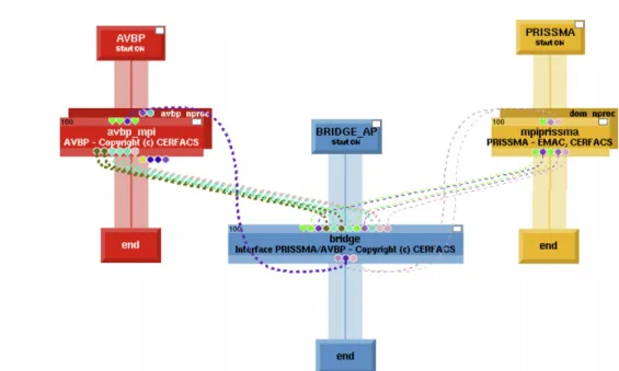
Fig. 1. The O-PALM interface. The different color dotted lines represent communicators between the solvers, including geometry, boundary conditions, temperature, pressure, mass fractions of absorbing species, etc. Colors are linked to the vector size. (For interpretation of the references to color in this figure legend, the reader is referred to the web version of this article.)
model SNB-FSCK with an S4 quadrature was used on the coarse mesh. This allowed to reach a CPU time ratio PRISSMA/AVBP close to one (i.e. with the same number of processors for LES and radia-tion: Nit# ( tLESCPU$=tCPURad) 0:6) and ensured CPU time
synchroniza-tion with an acceptable accuracy.
The data exchange, communications and resource distribution between PRISSMA and AVBP are handled by a coupler O-PALM,3
initially developed at CERFACS for meteorological applications[39]. It is used to run the two codes AVBP and PRISSMA on PLESand PRad processors respectively. A third code called ‘‘bridge’’ is used to han-dle the interpolation of physical data from AVBP to PRISSMA. The to-tal number of processors is P = PLES+ PRad+ 2, where two additional processors are used for the coupler driver and for the bridge (Fig. 2). The restitution time (i.e. wall clock time calculation for one solution) depends on the code efficiency and the allocated number of processors. AVBP is parallelized with a domain decomposition which is very efficient on massively parallel architectures with a perfect speed-up factor up to 4078 processors on IBM BlueGene/L
[40]. In the radiation calculation, the integral of the incident inten-sity involves the whole domain so that the use of domain decom-position is not straightforward. PRISSMA uses two levels of parallelism: directional and spectral. For an S4 quadrature with 15 spectral quadrature points, the maximum number of processors is 360, but the parallel efficiency is limited (around 30% for the maximum number of processors). This is an important limitation for coupled simulations on industrial configurations, and the use of domain decomposition for radiation is currently an issue that is under investigation.
Following the above strategy, the 132 processors of a SGI Altix ICE computer have been optimally distributed using 106 processors for AVBP, 24 for PRISSMA and 2 processors for O-PALM and the Bridge. This set-up gives a restitution time of 38.6 s for 100 itera-tions of AVBP and 37.2 s for PRISSMA, i.e. a well-balanced coupling.
3. Configuration 3.1. Geometry
The study case corresponds to an experiment developed and initially analyzed by Knikker et al.[41–43](Fig. 1). A premixed pro-pane/air flow is injected into a rectangular chamber, of dimensions 50, 80 and 400 mm in height, depth and length, respectively. Lat-eral walls are transparent and built with artificial quartz windows to allow visualization of the flame. The upper and the lower walls are made of ceramic material for thermal insulation and also include quartz windows to introduce LASER sheets for measure-ments (cf.Fig. 1).
A stainless steel triangular flame holder is fixed to lateral win-dows, measuring 25 mm in height which corresponds to a 50% blockage ratio. The V-shaped turbulent flame is stabilized by the flow velocity recirculating zone behind the flame holder.
Inlet conditions are given for the propane/air mixture with a velocity of 5 m s&1, a temperature of 300 K with an equivalent ratio of / = 1. Non-uniform mean profiles are imposed at the inlet, corresponding to fully developed turbulent channel flows. No turbu-lent fluctuations were added. Outlet condition is at atmospheric pressure.
3.2. Simulation set up
In the simulation, the inlet is placed 10 cm upstream the flame holder and the chamber is 30 cm long. A 3D box of 30 ( 30 ( 30 cm is added at the outlet of the chamber to emulate the atmo-sphere. The mesh contains about 4.7 millions tetrahedra. The cell size is about 1 mm, for the smallest cells close to the obstacle, and then increases progressively toward the exit of the chamber. To guarantee a non-disturbing outlet boundary condition, a nitrogen co-flow is added at the left-most limit of the atmosphere, thus avoid-ing recirculation in the computational domain and at the outlet. The co-flow has a velocity of 20 m s&1and the burnt gas temperature of 1900 K. This velocity is high enough to avoid outgoing flow but small enough to keep the main flow unchanged.
The walls of the chamber are not isothermal: the wall tempera-ture is the result of heat transfer through the solid between the inte-rior and the exteinte-rior of the chamber. In the present simulation, this is modeled using a wall thermal resistance of Rth= 0.096 K m2W&1for the ceramic walls (upper and lower), Rth= 0.086 K m2W&1for quartz windows (front and behind) and Rth= 120 K m2W&1for the flame holder[38]. The heat loss at the wall is calculated as:
qwall¼ 1
RthðTref& TwallÞ ð24Þ
with Tref= 300 K and Twallthe fluid temperature near the wall. The walls around the atmosphere at the end of the chamber are adia-batic slip walls.
In the radiative solver, the walls are however assumed isother-mal with Tw= 300 K except for the coflow which is at Tw= 1900 K. As discussed previously, this is not consistent with the thermal wall loss in the fluid solver, and the conduction in the solid should be calculated.
4. Results 4.1. Flow
LES results have been compared against experimental data in
[38]in terms of progress variable and a good agreement allowed to validate the LES simulation. The progress variable is a reduced Fig. 2. Stretch of the configuration[41].
quantity based on the temperature and is not suitable to evaluate radiation. Although LES and radiation computing were largely but independently validated in previous works [1–3,17–19], to the authors knowledge, simultaneous combustion and radiation mea-surements do not exist to validate both solvers together.
Mean fields were obtained after time averaging over 46.2 m s for the uncoupled solution and over 39.0 m s for the coupled calculation.
Figure 3shows the temperature and the velocity fields in the plane z = 0 for the LES calculation without radiation. The velocity fields show a recirculation zone behind the flame holder where the trapped hot gas stabilizes the flame. RMS fields show high
levels close to the wall caused by the flame quenching and reign-iting to consume the remaining unburnt fuel.
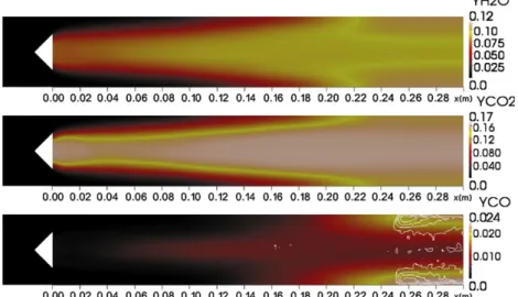
The time averaged fields of mass fractions of radiating species (H2O, CO2and CO) in the plane z = 0 are plotted inFig. 4. A large amount of CO is produced at the end of the chamber. The mass frac-tion of CO is more important than in adiabatic condifrac-tions due to the thermal wall law loss. As the second chemical reaction in Eq.(13)is reversible, the thermal losses shift the equilibrium backwards. The large amount of CO is localized where the second equilibrium (Eq.
(15)) is reversed. The contour observed on YCOinFig. 4represents the line where the net second reaction rate is zero. In the chemical mechanism used here, the second reaction is endothermic and was
Fig. 3. Fields of temperature and velocity in the plane z = 0 for the calculation without radiation: (a) Instantaneous. (b) Time averaged. (c) RMS.
Fig. 4. Time averaged fields of mass fraction of H2O (top), CO2(middle) and CO (bottom) in the plane z = 0 for the calculation without radiation. On the CO image, an isoline of
added to obtain the correct flame speed and burnt gas temperature of the laminar premixed flame under adiabatic conditions. A partic-ular attention must be paid to its use in non-adiabatic cases: in such situations, CO concentrations can highly deviate from the adiabatic reference in which the kinetic scheme was built.
4.2. Influence of radiation on turbulent combustion
Two LES calculations have been performed to evaluate the rela-tive influence of radiation on turbulent combustion: a LES stand alone simulation without radiation (called ‘‘uncoupled’’ in Eqs.
(25) and (26)) and a LES simulation fully coupled with the radiative solved to take into account the radiative source term in the LES en-ergy balance equation (called ‘‘coupled’’ in Eqs.(25) and (26)).
The total energy released by the combustion in the chamber in the calculation without radiation is 76.04 kW. The total net radia-tive energy is about 1.89 kW, i.e. only 2.48% of the combustion en-ergy. The radiative effect on the mean flow is therefore a second-order effect. However, previous studies[38]have shown that this effect may still be important, in particular by increasing the flow fluctuations. Note that the radiated energy is not equal to the heat release difference between the calculations with and without radi-ation, because the combustion chamber is not adiabatic: the outlet is not closed, and the gas in the combustion chamber exchanges radiative energy with the gas in the atmosphere.
Figure 5shows the mean heat release and the radiative source term fields in the plane z = 0. Although the energy released by com-bustion is much more important in intensity (by about 2 orders of magnitude), the spatial distribution strongly differs (see the ratio — Sr—/HR inFig. 5). The energy released by combustion is located along the flame front where the gas is burning while the radiative source term is important in non-reacting zones inside the burnt gas. Therefore, the impact of radiation strongly depends on the ra-tio between the flame surface and the volume of burnt gas.
The two-steps reduced chemistry was built and validated under adiabatic conditions. Using it in non-adiabatic conditions could be cautious and may be verified by looking at volume-averaged of the time-averaged quantities, given inTable 1 for both calculations with and without radiation, together with their relative difference. All are around 1%, confirming that heat losses are small and the re-duced chemistry may still be used in the non-adiabatic case. The total mass fraction of CO is modified by 10%, but such variation
should be considered with caution in this analysis: as already men-tioned, CO was introduced in the reduced chemical scheme to ob-tain the correct flame speed and temperature, but not the CO level, which may lead to non-physical values of CO mass fraction in the flame brush region. However, minor species are known to be more sensitive to the temperature level[44,24] and may be more im-pacted by radiation.
Looking now at local quantities absolute and normalized differ-ence fields are calculated for various mean variables and presented inFig. 6. For a quantity X, the absolute difference is defined as:
DðXÞ ¼ Xcoupled& Xuncoupled ð25Þ
while the normalized absolute difference is calculated as:
dðXÞ ¼Xcoupled& Xuncoupled
maxðXuncoupledÞ ð26Þ
Figure 6shows that radiation decreases the local temperature about 140 K near the flame front in the burnt gas side. In the fresh gas, the temperature is locally increased by more than 100 K. Tem-perature RMS values are compared using the intensity of tempera-ture fluctuations, defined as:
IðTRMSÞ ¼TRMS
eT ð27Þ
where eT is the filtered temperature. In both cases, the maximum temperature fluctuation intensity is around 85%. Taking into ac-count radiation, the absolute difference on the intensity fluctuations is decreased by 9.3% in burnt gas and increased by 7.5% around the flame front. Temperature is modified by radiation: the burnt tem-perature T1is decreased while the cold temperature T0is increased. The heat release factor
s
= (T1/T0) & 1 is decreased producing anFig. 5. Time averaged fields of heat release (top) and radiative source term (middle) and norm of the relative contribution of Sr compared to the heat release _xTðjSr= _xTjÞ in
percent with a contour at jSrj ¼ _xT(bottom, logarithmic scale) in the plane z = 0 for the calculation with radiation.
Table 1
Influence of radiation on total quantities integrated over the whole domain and relative difference between the two simulations.
Uncoupled Coupled Relative difference (%) YH2O 5.47 ( 10
&2 5.43 ( 10&2 &0.67
YCO2 9.36 ( 10&2 9.37 ( 10&2 0.12
YCO 5.19 ( 10&3 4.70 ( 10&3 &9.45 T(K) 1435.32 1417.27 &1.26 HR (kW/m3) 76.38 76.04
&0.45 P(Pa) 1.21 ( 105 1.22 ( 105 0.82
increase in the flame speed S0
l which enhances the flame sensitivity to turbulent motion.
The relative difference on the heat release shows that the max-imum energy released by combustion can be decreased on the flame front by more than 15%, but the flame brush is thickened by the inclusion of radiation. This is consistent with the increase of temperature fluctuations: the wrinkling of the flame front is lar-ger, so the mean reacting zone is thickened and the maximum time averaged value is decreased.
A very small impact is observed on the relative difference of velocity showing that the main dynamics of the flow is not altered
by radiation. However, the mass flux changes close to the flame front, due to dilatation of the gas in the zone where the tempera-ture is modified. In the cold gas, the mass flow rate is decreased by 8%, and in the burnt gas, it is increased by 4%. The impact on pressure is negligible.
The effect of radiation is limited on the mean dynamics of the flow, but is clearly visible on instantaneous solutions, as shown in Fig. 7 where fields of temperature and velocity at the same time for the calculations with and without radiation. The computation including radiation shows larger turbulent structures (i.e. lower spatial frequencies). A similar result was Fig. 6. Absolute (D(X)) and normalized (d(X) in %) differences between simulations with and without radiation for the time averaged temperature T, temperature intensity fluctuations I(TRMS), heat release _xT, velocity, mass fluxq( u and pressure P.
Fig. 7. Instantanous fields of temperature for the simulation without (top) and with (bottom) radiation at t = 0.5468817 s. On the top figure the probe location for the spectral analysis (x = 1, y = 1.5, z = 0 cm) is represented by a white square.
presented by Wu et al. [8], where radiation was included in a DNS calculation: the flame front was slightly thickened and spa-tial fluctuations became larger with radiation. In the present work, the use of the TFLES model makes it however difficult to measure an effect of larger spatial scales on the flame thick-ness. Frequency analysis using FFT of temporal signals requires very long simulations because the characteristic frequency of the flow is low. A frequency-time analysis is preferred using a wavelet approach which gives quantitative information on the unsteadiness of the flow and is shown inFigs. 8–11. The wave-let power spectrum calculated for the y-component of the veloc-ity is plotted inFigs. 8 and 9and for the temperature inFigs. 10 and 11. The calculation without radiation has two candidates for characteristic frequencies, the first in the range 128–256 Hz and a second in the range 256–512 Hz. For the available sampling time, these two frequencies alternate in time. When including radiation, the behavior of the system is different: the two fre-quency ranges are nearly merged. The lower frequencies are amplified as suggested by the instantaneous fields in Fig. 7. The temporal evolution of the high frequencies tends to be smoother when radiation is considered. This means that radia-tion modifies the turbulent distriburadia-tion of energy (i.e. turbu-lence diffuses energy at higher frequencies): indeed, radiation exchanges energy between hot and fresh gases and tends to
homogenize the energy distribution. This is a first step into the analysis of the influence of radiative heat transfer on flow instabilities and should be confirmed on other configurations using a larger sampling time. This would allow FFT analysis to give more quantitative information such as power spectral den-sities (PSD), able to show prominent peaks at the characteristic frequencies for unsteady regimes [45–48].
5. Influence of turbulence on radiation: Turbulence Radiation Interaction (TRI) analysis
The problem of the Turbulence Radiation Interaction has been studied for over two decades using theory, experiments and simu-lations and a detailed review on the subject has been written by Coelho[5]. When calculating the time averaged radiative source term, neglecting fluctuations can lead into large discrepancies due to the nonlinearity of the radiative source term. This is the so-called TRI problem; this question was firstly defined and treated in the Reynolds Average Navier–Stokes (RANS) context.
One of the main difficulties encountered in the analysis of TRI is to be able to collect realistic time and space fluctuations of the dif-ferent quantities describing combustion. Experimentally instanta-neous fields are difficult to obtain for all flow quantities, so numerical simulation has been widely used to generate them. In Fig. 8. Time–frequency wavelet power spectrum of the y-component of the velocity
in the calculation without radiation. Structures under black line are not representative.
Fig. 9. Time–frequency wavelet power spectrum of the y-component of the velocity in the calculation with radiation. Structures under black line are not representative.
Fig. 10. Time–frequency wavelet power spectrum of the temperature for the calculation without radiation. Structures under black line are not representative.
Fig. 11. Time–frequency wavelet power spectrum of the temperature in the calculation with radiation. Structures under black line are not representative.
first studies, some authors presumed the shape of the PDF to gen-erate temperature fluctuations[49,50]. Subsequently, there were attempts to generate fluctuations along the lines of sight[5].
LES explicitly solves large turbulent fluctuations while the smallest eddies are modeled: the unsteady quantities of the flow are decomposed in a filtered value and a fluctuating part:
X ¼ eX þ X0 ð28Þ
¼ hXi þ X|fflfflfflfflffl{zfflfflfflfflffl}00þX0 ð29Þ
where eX is the LES spatially filtered value, X0 is the subgrid scale fluctuation, hXi is the time-averaged value and X00 is the temporal fluctuation related to the filtered value.
In Eq.(29)the filtered value from LES (noted with a tilde) has been decomposed in a time averaged value and a fluctuating re-solved part (noted with a double prime). Therefore, it is possible to use LES to calculate explicitly all the TRI contributions over the whole domain using realistic resolved fluctuations (precedent studies [31,30,32–34] have shown that the influence of subgrid scale fluctuations X0could be neglected).
Only a few authors acknowledge the use of LES for TRI. Mala-lasekera et al.[51]used Discrete Transfer Method (DTM) with a Mixed Gray Gas Model to study a swirl jet flame of CH4/H2(1:1). They compared the TRI effects by time averaging LES results at four probe locations. Gupta et al.[52]also used LES to calculate TRI con-tributions with a P1-Gray model for radiation on non-reacting tur-bulent planar channel. They performed a sensitivity analysis of the TRI with the gray optical thickness.
In this work, a new approach is proposed: LES is used to explic-itly calculate all the TRI contributions over the whole domain, for a real turbulent flame configuration, using a detailed radiation mod-el (DOM) and an accurate global spectral modmod-el SNB-FSCK.
The radiative source term Srgiven by Eq. (16)can be decom-posed in two parts:
Sr¼ Sr;e& Sr;i ð30Þ
where Sr,eis the emitted energy and Sr,ithe incident energy, defined as: Sr;e¼ 4
rj
PðT; XiÞT4 ð31Þ Sr;i¼ Z 1 0j
m Gmdm
ð32Þwhere
j
pis known as the mean Planck absorption coefficient and G is the incident radiation integrated over the solid angle.The time averaged values of the flow quantities (e.g. tempera-ture T and species molar fraction Xi) are extracted from the simu-lation coupled with radiation. From this mean solution, the radiative fields of the mean flow are calculated: the radiative source term Sr(hTi, hXii), the incident radiative energy Sr,i(hTi, hXii), and the mean Planck absorption coefficient
j
P(hTi, hXii). This gives radiative fields where no turbulent fluctuation is included (like mean fields obtained from a RANS simulation).The differences between these radiative fields and mean radia-tive source terms (i.e. hSr(T, Xi)i), obtained from instantanous solu-tions of a simulation coupled with radiation, are due to the nonlinearities of the radiative source term which can be decom-posed as:
hSrðT; XiÞi ¼ Sr;eðhTi; hXiiÞð1 þ RjPÞð1 þ RT4þ RIbÞ
& Sr;iðhTi; hXiiÞð1 þ RGÞ – SrðhTi; hXiiÞ ð33Þ
where RjP; RT4; RIbcorrespond respectively to the absorption
coeffi-cient auto-correlation, the temperature auto-correlation and the cross-correlation between temperature and absorption. In addition, a new TRI quantity appears in the incident term, RG, corresponding to the absorption correlation. These correlations are defined as:
Rjp ¼jhPjðhTi;hXPðT;XiÞiiiÞ& 1
RT4¼hT 4 i hTi4& 1 RIb ¼ hj0 PðT4Þ0i hjPihTi4 9 > > > > = > > > > ; Emission TRI ð34Þ RG¼ShSr;iðT; XiÞi
r;iðhTi; hXiiÞ& 1 : Incident TRI ð35Þ
RSr¼ hS rðT; XiÞi
SrðhTi; hXiiÞ& 1 : Total TRI ð36Þ
In all these expressions, it was assumed that temporal and spectral integration are commutative. In the literature RjP, RT4, RGand RSrare
usually defined without the &1 term. In this work, all the correla-tions have been defined to represent only the turbulent part and are zero in laminar zones.
The correlations have been reconstructed using the unsteady cal-culation by performing temporal averaging of Sr, Sr,i,
j
P(Fig. 12) and T4. These values are computed from the radiative instantaneous solutions and take into account the effects of turbulence. In addition, an independent radiative calculation was carried out using a time averaged solution of the coupled LES solution with radiation. TRI quantities RjP, RT4and RGcan be directly deduced from these fields,and the cross-correlation RIbcan be reconstructed:
RIb ¼
hSr;eðT; XiÞi
Sr;eðhTi; hXiiÞ
1 1 þ RjP
& ð1 þ RT4Þ ð37Þ
The correlations calculated using Eqs.(34)–(36)are plotted in
Fig. 13. It is shown that absolute values of TRI reach important val-ues, up to 100%. However, absolute values are not representative of the influence of the TRI on the radiated energy: for example RGis more important beyond the flame holder than in burnt gases, as in this region gases are transparent and Sris weak. It is more con-venient to normalize TRI correlations with the maximum emitted, incident and total energy such as:
d Rjp ¼ Rjp d RT4¼ RT4 c RIb ¼ RIb 9 > > = > > ;
(maxhShSr;eðT; XiÞi
r;eðT; XiÞi ð38Þ
c
RG¼ RG(maxhShSr;iðT; XiÞi
r;iðT; XiÞi ð39Þ
c
RSr ¼ RSr( hS rðT; XiÞi
maxhSrðT; XiÞi ð40Þ
The total radiative heat loss is 1.89 kW when turbulence is in-cluded and 1.76 kW when it is not. This corresponds to the relative difference of 7.4%, but even if the difference on total heat loss is moderate, the distribution of Sr has variations from &20% to +20% as shown inFig. 14by RSr.
The correlation RT4 and RIb in Figs. 13 and 14 are the most
important correlations. They are located in the flame brush where the values of TRMSare high (Fig. 3). The first one is positive while the second is negative leading to an equilibrium between the two terms, as discussed in a preceding paper[31].
Following the analysis proposed by Snegirev[53], a Taylor expan-sion of
j
Pas a function of T and Xican be performed. If the fluctuation intensity is low, higher-order correlations may be dropped, and the emission correlations RT4and RIbmay be written as:RT4) 6hT 02i hT2i ð41Þ RIb ) 4 1 h
j
PðT; XiÞihTi hT 02i@j
P @T ! ** * * hTi þ hT0X0i@j
P @Xi * * * * hXii ! ð42ÞThe temperature auto-correlation is always positive (see Eq.(41)). The cross correlation can be positive or negative as it depends on a term in@jP
@T (Eq.(42)), which is mainly negative.
Figure 14shows that the absorption auto-correlation RjP and
the incident correlation RGare low (at the exception of the zone near the flame anchorFig. 14). These two correlations have also Fig. 12. Time averaged fields for Sr(isoline at Sr= 0), Sr,iand Kpin the plane z = 0.
Fig. 13. Turbulent correlations of the TRI: absorption auto-correlation RjP, temperature auto-correlation RT4, temperature-absorption cross correlation RIb, incident
an opposite effect and are linked because RGcontains a contribu-tion of the absorpcontribu-tion correlacontribu-tion (see Eqs. (35) and (32)). The net budget in Eq.(33)is positive as RjP P RG.
6. Application of TRI in the RANS context
Several approaches were developed for RANS applications to model the impact of TRI. The purpose is to reconstruct hSr(T, Xi)i from the mean values Sr(hTi, hXii) along with a model which de-scribes TRI. These approaches can be tested using the different cor-relations calculated with LES.
The most classical approximation to model TRI consists in neglecting RG using the so-called ‘‘Optically Thin Fluctuation Approximation’’ (OTFA) [54]. This is the most difficult term to model because it depends on non-local terms. So in this first ap-proach, all the emission TRI correlations (i.e. RjP; RT4 and RIb) are
considered, but the incident TRI (i.e. RG) is neglected.
In the literature, different levels of description are used to de-scribe emission TRI[5]: in the first level, (improperly) called ‘‘Full TRI’’, the absorption auto-correlation RjP is assumed to be weak
and only RT4 and RIbare kept; in the second level, called ‘‘Partial
TRI’’, only the temperature auto-correlation is evaluated.
Figure 15shows the relative error of the four approaches: OTFA only (RGis neglected), OTFA–Full (RGand RjPare neglected), OTFA–
Partial (only RT4is considered) and No TRI (all correlations are
ne-glected). The relative error between the TRI models and the full coupled simulation is calculated using:
!
TRI¼ Sr;eðhTi; hXiiÞhSr;eðT; XiÞi ( R & 1
! "
þ Sr;iðhTi; hXiiÞ hSr;iðT; XiÞi & 1
! "
( )
(maxhShSrðT; XiÞi
rðT; XiÞi ð43Þ
where the total correlation factor R is different for each model:
R ¼ ð1 þ RjPÞð1 þ RT4þ RIbÞ : OTFA only ð44Þ
R ¼ 1 þ RT4þ RIb : OTFA—\Full TRI" ð45Þ
R ¼ 1 þ RT4 : OTFA—\Partial TRI" ð46Þ
R ¼ 1 : No TRI ð47Þ
Relative errors fromFig. 15give the validity of each TRI model. As presented in Fig. 14, neglecting the incident TRI in the OTFA-Only approach gives errors around 10%. With the three other ap-proaches OTFA–Full, OTFA–Partial and No TRI, the errors are simi-lar showing that an uncomplete set of the emission TRI correlations (i.e. RjP; RT4 and RIb) is not sufficient.Table 2shows
the same result on total radiative loss. Moreover, the OTFA–Partial approach gives a higher error due to the unbalancing of the oppo-site contributions of RT4and RIb. The calculation of the total
radia-tive loss given inTable 2confirms these results.
TRI analysis inFigs. 13 and 14from LES results shows that each correlation contribution is important. The correlations RT4 and RIb
are slightly more important but RjP must not be neglected. The
incident correlation RGis slightly weaker but has the same order of magnitude than the other correlations. There are two compensa-tions mechanisms, first between RT4and RIband second between
RjPand RG. However, the net contribution on RSrremains important
close to the flame front and inside burning gases.
These results demonstrate the importance of radiative unsteady calculations even in cases where the modification of fluid dynam-ics caused by radiation is not studied. The temporal analysis of TRI from LES fluctuations shows that all the correlations are important and must be considered. Even more it shows that neglecting some terms can create an unbalance in the correlations leading to wrong radiative fields.
In RANS, the TRI correlations are calculated (or modeled) from RANS turbulence models[5]. In LES, it has been shown in this work that TRI correlations can be explicitly calculated from resolved fluctuations. This kind of analysis could also be used to build a Fig. 14. Scaled correlations of the TRI: absorption auto-correlation dRjP, temperature auto-correlation dRT4, temperature-absorption cross correlation cRIb, incident correlation
c
model for the TRI correlations in the computation of hSr(T, Xi)i using LES simulations instead of a RANS model.
7. Conclusions
A detailed study of the coupling between radiative heat transfer and LES of turbulent combustion in a real laboratory flame config-uration has been presented.
It was shown that radiation impacts the structure of the flame brush. Although the radiative energy is two orders of magnitude lower than the heat release by combustion, radiative exchanges have a visible impact on the energy distribution. Radiation has a higher ef-fect on local quantities compared to global quantities: the mean temperature in the domain decreases by 20 K with radiation, while extreme temperatures change between &150 K and +150 K (in-crease in fresh gas and de(in-crease in burnt gas). This can have a signif-icant effect on the prediction of minor species pollutants or soot and should be studied using detailed chemistry. These temperature changes have also an impact of the flame sensitivity to turbulent motion and increase of the flame fluctuations: the wrinkling of flame brush is stronger. The mean flow velocity is not altered, but a variation on mean flow rate, due to dilatation, was detected. The
un-steady evolution of the flow has been discussed using a time–fre-quency analysis with power spectrum wavelets. This analysis showed that peaks at characteristic frequencies are smoother and larger when radiation is present. Finally, radiation tends to homog-enize energy and frequency distribution of the flow.
The second part of the study focuses on the Turbulence Radia-tion InteracRadia-tion (TRI) using instantaneous radiative fields on the whole computational domain. For the first time, TRI correlations are calculated in a real burner using unsteady turbulent fluctua-tions obtained from LES. Results are in agreement with previous studies [5,8]and demonstrate the interest of using LES to study TRI in an a posteriori approach in a real burner configuration.
The results show that Turbulence Radiation Interaction in-creases the total radiative heat loss by 7.4% and that at some points, the radiative source term varies from &20% to +20%. The relative importance of each correlation has been discussed using four levels of approximation used in literature: OTFA-Only (RG ne-glected), OTFA–Full (RjP and RGneglected), OTFA–Partial (RjP; RIb
and RGneglected) and No TRI (all neglected), showing that all of the correlations have an important effect. This study shows that all three emission TRI must be considered, and the absorption auto-correlation cannot be neglected. The incident TRI RGis slightly less important but has the same order of magnitude than emission TRI. The TRI analysis is a first step towards TRI modeling in turbu-lent flames, and this work constitutes a good basis to build radia-tive models including the TRI correlations for RANS simulations. Acknowledgments
This work was granted access to the HPC resources of CINES under the allocation 2011-c2011026401 made by GENCI (Grand Equipement National de Calcul Intensif). We acknowledge Fig. 15. Evaluation of the different approaches developed in RANS context using correlations calculated from LES. OTFA: RGis neglected; OTFA+‘‘Full TRI’’: RGand RjPare
neglected; OTFA+‘‘Partial TRI’’: only RT4is considered; No TRI: all correlation are neglected.
Table 2
Influence of the RANS approaches on the total radiative loss.
Total radiative losses (kW) Relative difference (%) All correlations 1.89 –
OTFA 1.92 +1.64
OTFA+‘‘Full TRI’’ 1.80 &5.08 OTFA+‘‘Partial TRI’’ 2.07 +9.16 No TRI 1.76 &6.88
A. Dauptain form CERFACS for his help on the unsteady analysis and the calculation of wavelets.
References
[1] M. Boileau, G. Staffelbach, B. Cuenot, T. Poinsot, C. Bérat, Combust. Flame 154 (2008) 2–22.
[2] A. Roux, L. Gicquel, Y. Sommerer, T. Poinsot, Combust. Flame 152 (2008) 154– 176.
[3] G. Boudier, L. Gicquel, T. Poinsot, Combust. Flame 155 (2008) 196–214. [4] D. Poitou, M. El Hafi, B. Cuenot, J. Heat Transfer 133 (2010) 062701-10. [5] P.J. Coelho, Progr. Energy Combust. Sci 33 (2007) 311–383.
[6] M.F. Modest, Int. J. Multiscale Comput. Eng. 3 (2005) 85–106. [7] T.H. Song, R. Viskanta, J. Thermophys. Heat Trans. 1 (1987) 56–62. [8] Y. Wu, M.F. Modest, D.C. Haworth, J. Comput. Phys. 223 (2007) 898–922. [9] P. Sagaut, Large Eddy Simulation for Incompressible Flows: An Introduction,
Springer Science & Business, 2006.
[10] T. Poinsot, D. Veynante, Theoretical and Numerical Combustion, Edwards, 2001.
[12] F. Nicoud, F. Ducros, Flow Turb. Combust. 62 (1999) 183–200. [13] T. Poinsot, S. Lele, J. Comput. Phys. 101 (1992) 104–129. [14] O. Colin, M. Rudgyard, J. Comput. Phys. 162 (2000) 338–371.
[15] O. Colin, F. Ducros, D. Veynante, T. Poinsot, Phys. Fluids 12 (2000) 1843–1863. [16] L. Selle, G. Lartigue, T. Poinsot, R. Koch, K.-U. Schildmacher, W. Krebs, B. Prade,
P. Kaufmann, D. Veynante, Combust. Flame 137 (2004) 489–505.
[17] D. Joseph, P.J. Coelho, B. Cuenot, M.E. Hafi, Application of the discrete ordinates method to grey media in complex geometries using 3-dimensional unstructured meshes, in: P. Lybaert V. Feldheim, D. Lemonnier, N. Selcuk (Eds.), EUROTHERM73 on Computational Thermal Radiation in Participating Media, vol. 11, EUROTHERM, Faculté Polytechnique de Mons, Belgium, 2003, pp. 97–106.
[18] D. Joseph, M.E. Hafi, R. Fournier, B. Cuenot, Int. J. Therm. Sci. 44 (2005) 851– 864.
[19] K.A. Jensen, J. Ripoll, A. Wray, D. Joseph, M.E. Hafi, Combust. Flame 148 (2007) 263–279.
[20] D. Joseph, P. Perez, M.E. Hafi, B. Cuenot, J. Heat Transfer 131 (2009) 052701-9. [21] J.S. Truelove, Discrete–Ordinate Solutions of the Radiation Transport Equation,
Univ. of Newcastle, 1987.
[22] R. Koch, R. Becker, J. Quant. Spectrosc. Radiat. Transfer 84 (2004) 423–435. [23] A. Soufiani, J. Taine, J. Taine, Tech. Int. J. Heat Mass Transfer 40 (1997) 987–
991.
[24] F. Liu, H. Guo, G.J. Smallwood, M. El Hafi, J. Quant. Spectrosc. Radiat. Transfer 84 (2004) 501–511.
[25] V. Goutiere, F. Liu, A. Charette, J. Quant. Spectrosc. Radiat. Transfer 64 (2000) 299–326.
[26] V. GoutiFre, A. Charette, L. Kiss, Number. Heat. Transfer, Part B 41 (2002) 361– 381.
[27] A. Soufiani, E. Djavdan, Combust. Flame 97 (1994) 240–250.
[28] D. Poitou, J. Amaya, C. Bushan Singh, D. Joseph, M.E. Hafi, B. Cuenot, Validity limits for the global model FS-SNBcK for combustion applications, in:
Proceedings of Eurotherm83 – Computational Thermal Radiation in Participating Media III, 2009.
[29] F. Liu, M. Yang, G. Smallwood, H. Zhang, Evaluation of the SNB based full-spectrum CK method for thermal radiation calculations in CO2—H2O mixtures,
in: Proceedings of ICHMT, RAD04, Istanbul, Turkey, 2004.
[30] D. Poitou, ModTlisation du rayonnement dans la simulation aux grandes Tchelles de la combustion turbulente, Ph.D. thesis, Institut National Polytechnique de Toulouse, 2009.
[31] D. Poitou, M.E. Hafi, B. Cuenot, Turk. J. Eng. Environ. 31 (2007) 371–381. [32] M. Roger, C.B.D. Silva, P.J. Coelho, Int. J. Heat Mass Transfer 52 (2009) 2243–
2254.
[33] P.J. Coelho, Combust. Flame 156 (2009) 1099–1110.
[34] M. Roger, P.J. Coelho, C.B. da Silva, Int. J. Heat Mass Transfer 53 (2010) 2897– 2907.
[35] J. Amaya, O. Cabrit, D. Poitou, B. Cuenot, M.E. Hafi, J. Quant. Spectrosc. Radiat. Transfer 111 (2010) 295–301.
[36] F. Duchaine, A. Corpron, L. Pons, V. Moureau, F. Nicoud, T. Poinsot, Int. J. Heat Mass Transfer 30 (2009) 1129–1141.
[37] Y. Wang, Direct Numerical Simulation of Non-Premixed Combustion with Soot and Thermal Radiation, Ph.D. thesis, University of Maryland, 2005. [38] R. Gontalves dos Santos, M. Lecanu, S. Ducruix, O. Gicquel, E. Iacona, D.
Veynante, Combust. Flame 152 (2008) 387–400.
[39] T. Lagarde, A. Piacentini, O. Thual, Q.J. Roy, Meteorol. Soc. 127 (2001) 189–207. [40] G. Staffelbach, L.Y.M. Gicquel, T. Poinsot, Highly Parallel Large Eddy Simulations of Multiburner Configurations in Industrial Gas Turbines, Complex Effects in LES, Lecture Notes in Computational Science and Engineering, pp. 325–336.
[41] R. Knikker, D. Veynante, J. Rolon, C. Meneveau, Planar laser-induced fluorescence in a turbulent premixed flame to analyze large eddy simulation models, in: Proceedings of the 10th international Symposium on Applications of Laser Techniques to Fluid Mechanics, 2000.
[42] R. Knikker, D. Veynante, C. Meneveau, Proc. Combust. Inst. 29 (2002) 2105– 2111.
[43] C. Nottin, R. Knikker, M. Boger, D. Veynante, Symp. Combust. Proc. 28 (2000) 67–73.
[44] H. Guo, F. Liu, G. Smallwood, Ömer Gülder, Combust. Theor. Model. 6 (2002) 173–187.
[45] C.B. da Silva, I. Malico, P.J. Coelho, New J. Phys. 11 (2009) 093001.
[46] K. Biswas, Y. Zheng, C.H. Kim, J. Gore, Proc. Combust. Inst. 31 (2007) 2581– 2588.
[47] Y. Zheng, R.S. Barlow, J.P. Gore, J. Heat Transfer 125 (2003) 1065–1073. [48] M. Kounalakis, Y. Sivathanu, G. Faeth, J. Heat Transfer 113 (1991). [49] G. Cox, Combust. Sci. Technol. 17 (1977) 75–78.
[50] S. Burns, SANDIA Report, SAND99-3190, 1999.
[51] W. Malalasekera, M. Deiveegan, S. Sadasivuni, S. Ibrahim, Evaluation of turbulence/radiation effects using LES combustion simulation data, in: Proceedings of Eurotherm83 – Computational Thermal Radiation in Participating Media III, 2009.
[52] A.H. Gupta, M.F. Modest, J. Heat Transfer 131 (6) (2009) 061704. [53] A.Y. Snegirev, Combust. Flame 136 (2004) 51–71.