HAL Id: hal-02316361
https://hal.archives-ouvertes.fr/hal-02316361
Submitted on 25 Oct 2019
HAL is a multi-disciplinary open access
archive for the deposit and dissemination of
sci-entific research documents, whether they are
pub-lished or not. The documents may come from
teaching and research institutions in France or
abroad, or from public or private research centers.
L’archive ouverte pluridisciplinaire HAL, est
destinée au dépôt et à la diffusion de documents
scientifiques de niveau recherche, publiés ou non,
émanant des établissements d’enseignement et de
recherche français ou étrangers, des laboratoires
publics ou privés.
Frequency dependence of the UWB indoor propagation
channel
Patrice Pajusco, Pascal Pagani
To cite this version:
Patrice Pajusco, Pascal Pagani. Frequency dependence of the UWB indoor propagation channel.
EuCAP 2007 : the second european conference on antennas and propagation, Nov 2007, Edinburgh,
United Kingdom. �hal-02316361�
FREQUENCY DEPENDENCE OF THE UWB INDOOR
PROPAGATION CHANNEL
P. Pajusco*, P. Pagani
†* France Telecom / Orange Labs, 6 avenue des Usines, 90000 Belfort, France
†
France Telecom / Orange Labs, 4 rue du Clos Courtel, 35510 Cesson Sévigné, France Email: {patrice.pajusco ; pascal.pagani}@orange-ftgroup.com
Keywords: Ultra-wideband; radio wave propagation; channel
characterization; frequency dependence.
Abstract
Ultra wideband (UWB) is seen as a major technology for future high rate, short range radio links. For the development of UWB-based communication systems for indoors, an accurate knowledge of the propagation channel is necessary. However, most of the available studies regarding the UWB radio channel concentrate on the lower frequencies of the FCC-defined spectrum mask, and experimental data is generally missing for the evaluation of the frequency dependence of the channel parameters. In this paper, an extensive sounding campaign is presented, where the UWB channel is probed from 3.1 GHz to 11.1 GHz in a typical indoor environment. Following a thorough analysis of the effect of the antennas on the measured data, a characterisation of the main propagation parameters is presented, with a specific interest on their frequency dependence. A frequency power decay close to the theoretical loss of 20 dB per decade is observed. Other typical parameters, such as the environment dependent path loss exponent, the delay spread or the power delay profile decay exponent show limited variations with increasing frequency. This behaviour may be explained by the characteristics of the main building materials constituting indoor environments, which present a relative stability in the frequency range of interest.
1 Introduction
UWB is a promising technology for short range telecommunication systems, consisting of transmitting signals over a wide frequency band, typically in the order of 500 MHz to several GHz [1]. In 2002, the Federal Communications Commission (FCC) released its first Report and Order, allowing the use of UWB signals in the 3.1 GHz – 10.6 GHz band [2]. A number of applications are currently envisioned, providing high data rates for data transfer using low cost terminals ([1], [3]). A large amount of research on the physical layer has thus been done for a few years. In order to develop efficient transmission systems, one of the main issues is to establish a realistic propagation channel model. Such a model is expected to accurately reproduce the key effects of an UWB radio link, such as the temporal selectivity, the spatial and temporal fading, and the effect of people moving in the vicinity of the terminal.
UWB channel modelling is generally based on the analysis of experimental data, allowing for the characterization of the
main channel parameters [4]. Accordingly, a number of UWB propagation experiments have been carried out since the appearing of this technology in the field of telecommunication ([5], [6]). Nevertheless, these propagation experiments are usually restricted to the lower part of the FCC-defined band. Only a few analyses focus on the whole UWB band extending from 3.1 GHz to 10.6 GHz ([7]-[10]). Thus, further investigations on the UWB channel are required, especially regarding the impact of the frequency. This paper presents an experimental analysis of the influence of the frequency on the different characteristics of the UWB propagation channel. For this purpose, we studied the indoor radio channel over the global 3.1 GHz – 10.6 GHz band, and on 7 partial bands of 528 MHz each, which corresponds to the bandwidth selected for the UWB systems standard ECMA-368 [11]. Section 2 describes the experiment performed in a typical indoor environment. The influence of the antenna on the measurement results is then analysed in Section 3. The two next sections are respectively dedicated to propagation loss results (Section 4) and to the study of large scale parameters in the delay domain (Section 5).
2 Experiment description
2.1 General measurement setupPropagation channel measurement can be performed in either temporal or frequency domains. Due to the ease and advantages of its implementation, we chose a sounding technique in the frequency domain using a Vector Network Analyser (VNA) HP8510C. The Channel Transfer Function (CTF) H(f) was thus obtained using standard S21 parameter
measurements. The propagation channel was sampled over 4005 equally spaced frequencies between 3.1 and 11.1 GHz. Hence, the whole FCC-defined frequency band for indoor UWB applications was probed. This setup allowed a maximum excess delay of about 500 ns and a temporal resolution of about 125 ps.
Conical Monopole Antennas operating in the 1 GHz – 18 GHz band (CMA 118) were used at each side of the radio link. The transmitting (Tx) antenna was mounted on a trolley to simplify the displacement to the different measurement locations. Depending on the configuration between the transmitter and the receiver, we used up to three Low Noise Amplifiers (LNA), with respective gains of 20 dB, 28 dB and 38 dB. The three LNA present a constant gain over the measured frequency band, and their transfer function was subtracted from the channel measurement at the calibration stage. A step motor enabled the displacement of the Tx
antenna along a circle of 40 cm in diameter. For each measurement, 90 complex CTF were measured at regular intervals along the circular path. This setup enabled evaluating the local variations of the UWB propagation channel.
The receiving (Rx) antenna was settled on a wall at a height of about 2 meters above the floor. Due to the asymmetry of the antenna pattern, the antenna was mounted upside down. This antenna was placed next to the VNA to minimise the loss of the received signal. The other port of the VNA was connected to the Tx antenna with a long and low loss cable. The maximum Tx-Rx distance was limited to 20 m. The whole measurement process (calibration, antenna rotation, video capture and data saving) was automated using a specifically developed MatlabTM software. The schematic diagram of our measurements is depicted in Fig. 1.
2.2 Environment description
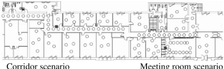
Measurements were performed in a typical indoor office environment, as depicted on Fig. 2. Two indoor office configurations were investigated. In the first scenario, the "access point" was located in a meeting room at a height of 2.19 m. In the second one, the "access point" was located in a corridor at a height of 2.45 m. In both cases, Line-Of-Sight (LOS) and Non Line-Of-Sight (NLOS) measurements were performed. The distance between transmitter and receiver varied from 1 m to 20 m. The trolley supporting the Tx antenna was placed at more than 120 locations, of which one third corresponded to a LOS configuration and two thirds to a NLOS configuration. At each location, 90 measurements were performed using the rotating arm, leading to a total of over 10 000 UWB CTF.
2.3 Data processing
During the propagation experiment, raw data from the VNA were stored in files. The measurement data was then calibrated with respect to a reference measurement where the emitter and the receiver were directly cable-connected. For measurements involving an LNA, the LNA transfer function was subtracted from the measurement at this stage. Several parameters were then extracted, by considering different bandwidths and central frequencies. First, the set of parameters was computed over the whole FCC-defined band (3.1 GHz – 10.6 GHz). Then, the same set of parameters was computed over 7 partial bands of 528 MHz each, which corresponds to the bandwidth specified by the UWB systems standard ECMA-368 [12]. The central frequencies of the selected bands extended from 4 GHz to 10 GHz with a 1 GHz step. As a result, it was possible to analyse the effect of the
central frequency on the characteristics of the UWB propagation channel. Most of computed parameters are recapped hereafter.
Each measurement being performed in the frequency domain, the measured quantity is the CTF H(f). Note that the CTF represents the joint effects of the channel and of the antennas, the influence of the sounding equipment being removed through the calibration procedure. How the antenna effect is treated will be explained in details in Section 3.
The average Power Transfer Function (PTF) was obtained by averaging the power of different co-located CTF along the measurement circular path:
( )
∑
( )
==
M m mf
H
M
f
PTF
1 21
(1) where M = 90 represents the number of co-located measurements, m represents the measurement index and Hm(f)is the corresponding CTF. Due to the CTF calibration, the PTF merely represents the average channel power attenuation for each measured frequency. The PTF was then used to compute the UWB Propagation Loss (PL) for a given central frequency fc in the measured band and a given observation
bandwidth BW, according to the following formula.
( )
∑
( )
+ < − >=
2 21
n c BW BW c n f f f f n c BWPTF
f
N
f
PL
(2)where N represents the number of measured frequencies fn in
the considered bandwidth.
To compute time domain parameters, the Channel Impulse Response (CIR) h(τ) is obtained from the CTF using an inverse Fourier transform.. A Hanning window was applied at this stage to reduce the side lobe level. The Power Delay Profile (PDP) was deduced using a power average, as follows:
( )
∑
( )
==
M m mh
M
PDP
1 21
τ
τ
(3)where the notations M and m are the same as in equation (1). The decreasing slope of the PDP was fitted to the following exponential approximation, using a least squares method:
γ τ
τ
≅
B
e
−PDP
(
)
2.
(4)where γ represents the PDP decay exponent, and B is a normalising constant.
The mean delay τm and the delay spread τRMS were finally
computed according to the following equations:
( )
( )
∫
∫
∞ + ∞ − +∞ ∞ −⋅
=
τ
τ
τ
τ
τ
τ
d
PDP
d
PDP
m (5) PC VNA - HP 8511110 CMA 118 CMA 118 P1 P2 RS232 GPIB Long cable LNA LNA LNAFigure 1: Schematic diagram of the measurement device.
Corridor scenario Meeting room scenario
Figure 2: Measurement locations for the UWB channel experiment. White circles represent emitter locations and shaded squares represent receiver locations.
(
)
( )
( )
∫
∫
∞ + ∞ − +∞ ∞ −−
⋅
=
τ
τ
τ
τ
τ
τ
τ
d
PDP
d
PDP
m RMS 2 (6)Figures 3 and 4 provide typical examples of measured PDP in LOS and NLOS configurations.
3 Antenna analysis
3.1 General descriptionWhen the radio channel is sounded over a frequency range representing more than an octave, the antenna may severely affect the measurements. The power received via each multipath impinging the Rx antenna depends directly on the antenna radiation pattern. Thus, if the antenna pattern is modified, the apparent channel properties may fluctuate accordingly. For instance, a narrow beam antenna focuses the transmitted energy on the direct path and the effect of the multipath components will therefore be attenuated. To minimize the influence of the antenna, we selected the CMA 118 antenna which presents an omni-directional radiation pattern and is vertically polarized. A picture of the antenna and its orientation are presented in Fig. 5.
In order to precisely assess the effect of the antennas used for the experiment, both Tx and Rx antennas were characterized in 3 dimensions (3D) in an anechoic chamber. The radiation
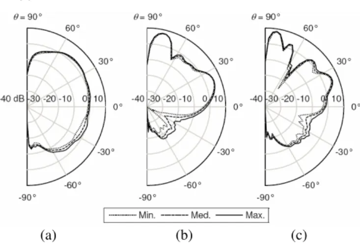
patterns of the two antennas are quite similar. However, in spite of the high quality of this product in terms of gain flatness over the measurement bandwidth, we observed a noticeable variation of the antenna characteristics as the frequency increases. As an example, Fig. 6 depicts the 3D antenna pattern measured at three selected frequencies within the FCC-defined frequency band. We can notice that the radiation pattern becomes less and less omni-directional in the elevation plane as the frequency increases. To evaluate the omni-directional behaviour of the antenna in the horizontal plane, we computed the minimum, the median and the maximum antenna gain in azimuth for each elevation. Figure 7 depicts the results obtained for the three frequencies taken as examples in Fig. 6. One can observe that the radiation pattern is relatively constant in azimuth for a given elevation and a given frequency.
Figure 3: Example of average Power Delay Profile in LOS configuration.
Figure 4: Example of average Power Delay Profile in NLOS configuration. x y z θ φ o x y z θ φ o
Figure 5: Reference axis and picture of the antenna CMA 118.
(a) (b) (c)
Antenna gain (dBi)
-20 -15 -10 -5 0 5
Figure 6: Examples of measured radiation patterns of the antenna CMA 118 at 3 GHz (a), 7 GHz (b) and 10 GHz (c).
(a) (b) (c)
Figure 7: Dispersion of the antenna CMA 118 radiation pattern in azimuth. Minimum, median and maximum antenna gain in azimuth for each elevation θ, at 3 GHz (a), 7 GHz (b), and 10 GHz (c).
3.2 Influence of the antennas on path loss
a) Distance domain
To evaluate the influence of the antenna on the distance dependent path loss, we consider a typical LOS configuration, as depicted in Fig. 8. In a typical sounding experiment, we normally expect a more severe channel attenuation when the Tx-Rx distance increases. However, an increasing distance also leads to a decrease of the elevation angle θ. Hence, the observed attenuation is not only due to changes in the length of the direct path, but also to variations of the antenna pattern with elevation. In our experiment, measurements were performed for distances ∆x varying from 1 m to 20 m. With a height difference ∆y of about 90 cm, the elevation θ varied between 3° and 42°. Figure 7 shows for three demonstrative frequencies that in this region, the radiation pattern presents small, but not negligible fluctuations. Depending on the Tx-Rx distance and on the frequency, the global variation of the direct path power due to the Tx and Rx antennas may be significant, in the order of 10 dB. Thus, the effect of the non-ideal antenna needs to be removed from the channel measurement. Otherwise, the antennas may introduce apparent fluctuations in the path loss parameters.
b) Frequency domain
In an ideal, free-space configuration, the propagation loss PL in dB between the transmitted and received power is given by Friis' formula:
(
)
G
( )
f
G
( )
f
c
d
f
d
f
PL
−
Tx−
Rx
⋅
⋅
⋅
=
20
log
4
π
,
(7)where f represents the frequency in Hz, d represents the Tx – Rx distance in m, GTx and GRx represent the Tx and Rx
antenna gains in dBi, and c is the speed of light. Equation (7) implies that for a given distance d, the channel average PTF (in linear scale) should be proportional to f -2. Noteworthy frequency power decay has been observed on previous UWB channel measurements ([8, 9, 13]). In [8], the channel power attenuation was observed to be proportional to kf
f
− , with kfvarying between 1.6 and 2.8. Reference [9] proposed a rather different approach, by fitting the measured PTF in dB to an exponential law.
When considering frequency power decay, one should keep in mind that the frequency term
20 ⋅
log
( )
f
in Friis' formula is related to the effective aperture of an ideal, isotropic antenna,while the characteristics of the real antennas are taken into account in the gains GTx and GRx. PTF measurements
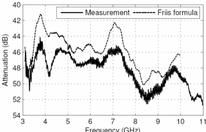
performed with non-ideal antennas are hence highly sensitive to the antenna patterns. Figure 9 illustrates this dependency by representing a PTF measured in a LOS configuration, along with the theoretical path loss computed from equation (7), where the gains GTx and GRx were measured in an
anechoic chamber at an elevation corresponding to the measurement situation. One can observe the predominant effect of the antennas, as the general shape of the measured PTF faithfully follows the variations of the antenna gains. Again, this result shows that the effects of non-ideal antennas should be taken into account prior to the computation of the channel characteristics.
4 Propagation loss results
4.1 Frequency dependent path lossIn order to assess the frequency dependent power decay linked to a channel using theoretical isotropic antennas, we studied the experimental values of the channel path loss at regularly spaced frequencies between 4 GHz and 10 GHz. For each measurement location, the pathloss
PL
(
f
,
d
)
was extracted at the frequencies of interest from the measured PTF. In order to remove the distance dependency, each PTF was initially normalised, by arbitrarily setting the attenuation of the total received power over the whole measurement bandwidth to 0 dB. The resulting normalised path loss( )
f
PL
norm could then be fitted to a linear approximation of the type:( )
( )
S( )
f f f k f PL f PLnorm norm f + ⋅ ⋅ + = 0 0 10 log (8)where kf represents the frequency power decay exponent, f0 is
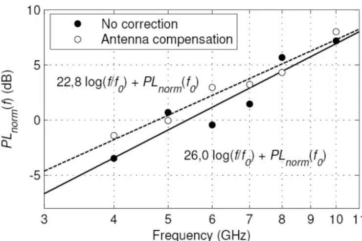
the central frequency and S(f) accounts for the fluctuations of the experimental data around the linear approximation. The normalised path loss averaged over all measurement locations is represented against frequency in Fig. 10. At first, no antenna correction was applied (black dots). One may note an increase of the path loss with increasing frequency, but there is no way to distinguish between the frequency dependent power decay and variations due to the antenna pattern. The computed power decay exponent is kf = 2.60,
Figure 8: Antennas configuration during the experiment. ∆x, ∆y and d respectively represent the horizontal, vertical and effective distances between the antennas, and θ is the elevation angle of the direct path.
leading to a standard deviation of the measured data around the linear approximation of 1.2 dB. Secondly, the measured antenna gains GTx(f) and GRx(f) were subtracted from the
measured PTF at each frequency of interest prior to path loss calculation (white dots). The antenna gain was selected by taking the direction of the direct Tx-Rx path into account. This approach may seem simplistic, as the total power is not received via the direct path only, but it allows a sensible compensation of the antenna effect, leading to satisfactory results: in this case, the dispersion of the measured plots around the linear approximation is reduced to a standard deviation of 0.6 dB. The frequency dependent power decay kf
falls to 2.28. With respect to the error level inherent to the measurement and computation methods, this value may be considered close to the theory. Hence, we recommend using the theoretical frequency loss of
20 ⋅
log
( )
f
in the modelling of UWB channels, which correspond to the theoretical effect of ideal, isotropic antennas.4.2 Distance dependent path loss over the FCC band
In this paragraph, we analyse the propagation loss parameters on the global FCC-defined frequency band extending from 3.1 GHz to 10.6 GHz. As observed in Section 4.1, a frequency loss of
20 ⋅
log
( )
f
accounting for ideal, isotropic antennas may be assumed. Section 3 also pointed out that the real antennas used during the experiment could adversely affect propagation loss analyses in both frequency and distance domains. Hence, the collected data was corrected to the possible extent, by removing the gain of both antennas, measured at the central frequency of the analysed band, with an angular elevation corresponding to the direction of the Tx-Rx path. Note that for the global UWB frequency band, the measurement performed at each frequency was corrected using the nearest measured radiation pattern. The resulting path loss in dB was fitted to the general formula in the form:(
)
(
)
( )
d S d d k f f d f PL d f PL d + ⋅ + ⋅ + = 0 0 0 0 log 10 log 20 , , (8)where kd is the environment dependent path loss exponent, d0
is an arbitrary distance of 1 m, f0 is the central frequency of
6.85 GHz, and S is the shadowing in dB, with zero mean and standard deviation σS.
Figure 11 depicts the path loss results for the global UWB frequency band, i.e. 3.1 GHz – 10.6 GHz. The measurement plots mainly follow a linear decay in log-scale, which corresponds to an exponential decay of the received power with respect to the distance. The parameters kd, PL(f0, d0) and
σS were computed by linear regression using a least squares
method. In the LOS case, a path loss exponent kd = 1.62 was
recorded, with a standard deviation σS = 1.7 dB. In the NLOS
case, the measurement plots are somewhat more dispersed, leading to a value of kd = 3.22, with a standard deviation
σS = 5.7 dB. These values are slightly lower but in the range
of the UWB path loss exponents computed from other measurements in an indoor environment [6, 7]. The value of PL(f0, d0) was respectively evaluated at 53.7 dB in the LOS
case and 59.4 dB in the NLOS case.
4.3 Frequency dependence of the path loss parameters
A few results only are available in the literature about the frequency dependence of the path loss exponent. An increase of kd with frequency is suggested in the NLOS case in [14].
Reference [11] reports a marked increase of the path loss exponent in the LOS case, while NLOS measurements exhibit the opposite trend. Hence, more experimental analysis was required on this subject.
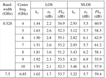
Table 1 summarizes the values obtained for kd, σS and
PL(f0, d0) when derived from the seven partial bands of
528 MHz each. The path loss exponent kd varies between 1.44
and 1.92 in the LOS case and between 2.82 and 4.21 in the NLOS case. As a global observation, the path loss exponent is relatively stable. Slightly higher values may be detected at high frequencies (8 GHz to 10 GHz). This small increase may arise from a variation in the characteristics of the building material in the vicinity of the radio link, but no regular trend is observable. The parameters σS and PL(f0, d0) do not appear
to be affected by the central frequency of the observed band. Measurement results presented in [15] indicate that the complex permittivity of concrete and plasterboard are relatively stable over the whole band defined for UWB communications. Similarly, reference [16] reports reasonably Figure 10: Average normalised path loss vs. frequency. Figure 11: Scatter plot of the power attenuation vs. distance.
low variations of the transmission loss measured for concrete and wood between the lower and upper frequencies of the UWB spectrum (less than 2 dB). These building materials constitute most of the walls in our measured environment. It is thus not surprising to observe a relative stability in the propagation properties of the UWB radio channel with respect to the frequency. Furthermore, one should note that all measurements were performed on a single floor. Inter-floor measurements involve possible wave propagation through reinforced concrete slabs, where the regular metallic netting could introduce frequency dependencies in the received signal. This was not the case in our experiment.
5 Large-scale delay domain results
5.1 Delay spreadThe delay spread τRMS was computed from each collected
PDP, over the whole FCC-defined band (3.1 GHz – 10.6 GHz). A threshold of 20 dB below the maximum value of the PDP was used to select the significant delays only and avoid the effect of noise. Over all measurement locations in a LOS configuration, the average value of the delay spread was τRMS = 4.1 ns with a standard deviation στ = 2.7 ns. In the
NLOS configuration, the average delay spread was τRMS = 9.9 ns with a standard deviation στ = 5.0 ns. These
figures agree with the values generally reported in the literature on UWB measurements [6].
In order to observe the evolution of these parameters with frequency, the average value of τRMS computed for seven
partial bands of 528 MHz each are plotted against central frequency in Fig. 12. For each band, the value of στ is
represented by the length of the vertical line. No frequency dependence of the RMS delay spread is noticeable. The values of τRMS and στ obtained in each 528 MHz-wide
frequency band are relatively close to the values observed for the global band extending from 3.1 GHz to 10.6 GHz.
5.2 Power Delay Profile
Figures 3 and 4 present typical PDPs in LOS and NLOS configurations. Note that for the convenience of path
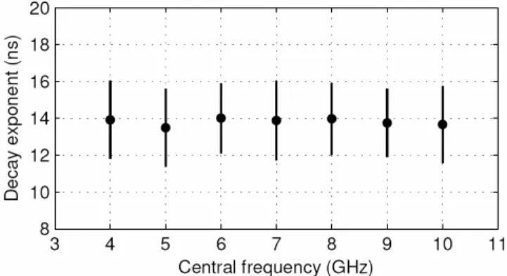
interpretation, the delay on the horizontal axis has been converted in path length in meters. In both LOS and NLOS cases, one may observe one or several clusters, corresponding to a main path followed by an exponential decay of diffuse power. In the LOS case, walls or pieces of furniture in the vicinity of the radio link produce strong reflected or diffracted echoes, which explains the presence of peaks in the PDP. The global shape of the PDP is generally smoother in the NLOS case, however multiple clusters may occasionally appear. The slope of the PDP exponential decay has been computed for each measurement location as explained in section 2.3. The decay exponent γ was separately computed for the whole FCC-defined band and for the seven partial bands of 528 MHz width each. Over the global band ranging from 3.1 GHz to 10.6 GHz, the average value of the decay exponent was γ = 15.1 ns with a standard deviation of σγ = 3.8 ns. From
the wide range of experimentally observed values [6, 7], this parameter seems highly environment dependent, and more research should be concentrated on this issue.
Figure 13 presents the average values of the PDP decay exponent obtained for seven bands of 528 MHz each, with different central frequencies. The corresponding standard deviations are represented by the length of the vertical lines. Clearly, there is no dependence of the decay exponent on the central frequency of each band, as the observed values are similar for all considered partial bands.
6 Conclusion
In this paper, we presented an exhaustive measurement campaign designed in the 3.1 GHz – 11.1 GHz frequency band to characterise the UWB indoor propagation channel. The main purpose was to evaluate the impact of frequency on the channel main parameters. Using a VNA and two antennas CMA 118, over 10 000 channel transfer functions were collected in both LOS and NLOS configurations. Despite the high quality of the antenna specifications in terms of gain flatness across the band, we demonstrated that the non-ideal antenna pattern could adversely affect the measured data in both frequency and distance domains. Hence, the antenna characteristics need to be precisely measured and removed to the possible extent from the raw collected data. This
LOS NLOS Band-width (GHz) Center freq. (GHz) kd σS (dB) PL0 (dB) kd σS (dB) PL0 (dB) 4 1.44 2.2 54.9 2.93 5.5 60.9 5 1.63 2.6 52.3 3.12 5.7 58.5 6 1.50 2.8 55.1 2.82 6.1 62.9 7 1.51 2.6 53.2 2.93 5.7 61.2 8 1.81 3.6 51.2 3.43 6.2 58.1 9 1.92 2.3 53.5 4.21 6.9 55.9 0.528 10 1.91 2.1 52.3 3.46 6.3 57.9 7.5 6.85 1.62 1.7 53.7 3.22 5.7 59.4 Table 1: Distance dependent path loss parameters for different
frequency bands.
Figure 12: Average RMS delay spread and standard deviation vs. central frequency.
technique was validated through the computation of the frequency dependent power decay: after correction of the antenna effects, the channel frequency loss was shown to approach the theoretical loss of 20 dB per decade. On a modelling point of view, this corresponds to using ideal, isotropic antennas. The effect of the practical antennas with respect to this theoretical case should be modelled separately, and added in the simulation chain for a realistic reproduction of the global radio link.
The main channel parameters were extracted over the global FCC-defined frequency band, extending from 3.1 GHz to 10.6 GHz. A decrease of the received power with increasing distance was observed, with an average path loss exponent of 1.62 in the LOS case and 3.22 in the NLOS case. The measured PDP generally presented a clustering of the multipath components, with respective average delay spreads of 4.1 ns and 9.9 ns in the LOS and NLOS cases, and an average decay exponent of 15.1 ns. When computed from several partial bands of 528 MHz each at different central frequencies, these parameters showed no or little impact of the frequency. A slight increasing trend of the path loss exponent with increasing frequency could be observed, but this topic needs further research for validation. As a general observation, a constant behaviour of the channel may be assumed over the whole UWB frequency band, in addition to the abovementioned frequency power decay. Using the adequate frequency dependent path loss formula, models based on measurements performed in the lower part of the UWB spectrum could thus be easily generalised to higher central frequencies. This conclusion comes in line with published results on the transmission coefficients of the main building material in indoor environments, which presented a relative stability across the FCC-defined frequency spectrum for UWB devices.
References
[1] L. Yang and G. B. Giannakis, “Ultra-wideband communications: an idea whose time has come”, IEEE Signal Processing Magazine, 21, pp. 26-54, (2004). [2] FCC, “First report and order, revision of Part 15 of the
Commission's rules regarding ultra-wideband transmission systems”, FCC ET Docket 98-153, (2002). [3] D. Porcino and W. Hirt, “Ultra-wideband radio
technology: potential and challenges ahead”, IEEE Communications Magazine, 41, pp. 66-74, (2003). [4] F. Molisch, J. R. Foerster, and M. Pendergrass,
“Channel models for ultrawideband personal area net-works”, IEEE Wireless Communications, 10, pp. 14-21, (2003).
[5] Z. Irahhauten, H. Nikookar, and G. J. M. Janssen, “An overview of ultra wide band indoor channel measurements and modeling”, IEEE Microwave and Wireless Components Letters, 14, pp. 386-388, (2004). [6] F. Molisch, K. Balakrishnan, C. Chong, et al., “IEEE
802.15.4a channel model - final report”, IEEE P802.15 Working Group for WPANs, Technical Report IEEE P802.15-04/0662r1-SG4a, (2004).
[7] J. Kunisch and J. Pamp, “Measurement results and modeling aspects for the UWB radio channel”, IEEE Ultra Wideband Systems and Technologies, Baltimore MD, USA, (2002).
[8] Alvarez, G. Valera, M. Lobeira, et al., “New channel impulse response model for UWB indoor system simulations”, IEEE Vehicular Technology Conference, Seoul, Korea, (2003).
[9] R. M. Buehrer, W. A. Davis, A. Safaai-Jazi, et al., “Characterization of the ultra-wideband channel”, IEEE Ultra Wideband Systems and Technologies, Reston VA, USA, (2003).
[10] D. Cassioli, A. Durantini, and W. Ciccognani, “The role of path loss on the selection of the operating bands of UWB systems”, IEEE International Symposium on Personal, Indoor and Mobile Radio Communications, Barcelona, Spain, (2004).
[11] ECMA International, “High Rate Ultra Wideband PHY and MAC Standards”, standard no. ECMA-368, (2005). [12] D. Cheung and C. Prettie, “A Path Loss Comparison
Between the 5 GHz UNII Band (802.11a) and the 2.4 GHz ISM Band (802.11b)”, Intel Corporation Technical Document, (2002).
[13] B. M. Donlan, S. Venkatesh, V. Bharadwaj, et al., “The ultra-wideband indoor channel”, IEEE Vehicular Technology Conference, Milan, Italy, (2004).
[14] R.-R. Lao, J.-H. Tarng, and C. Hsiao, “Transmission coefficients measurement of building materials for UWB systems in 3 -10 GHz”, IEEE Vehicular Technology Conference, Seoul, Korea, (2003).
[15] Muqaibel, A. Safaai-Jazi, A. Bayram, et al., “Ultra wideband material characterization for indoor propagation”, IEEE Antennas and Propagation Society International Symposium, Columbus OH, USA, (2003). [16] P. Pagani, P. Pajusco, and S. Voinot, “A Study of the
Ultra-Wide Band Indoor Channel: Propagation Experiment and Measurement Results”, International Workshop on Ultra Wideband Systems, Oulu, Finland, (2003).
[17] S. S. Ghassemzadeh, R. Jana, C. W. Rice, et al., “A statistical path loss model for in-home UWB channels”, IEEE Conference on Ultra Wideband Systems and Technologies, Baltimore MD, USA, (2002).
Figure 13: Average decay exponent and standard deviation vs. central frequency.