Simulation of spatial and temporal trends in nitrate concentrations at the regional scale in the Upper Dyle basin, Belgium

Texte intégral

(1)1. Simulation of spatial and temporal trends in nitrate concentrations at the regional. 2. scale in the Upper Dyle Basin, Belgium’. 3 1,*. 4. 1. 1. 2. 1. 1. César E. , Wildemeersch S. , Orban Ph. , Carrière S. , Brouyère S. , Dassargues A.. 5. 1. 6. Sart-Tilman, 4000 Liege, Belgium. 7. 2. 8. 84 000 Avignon, France. 9. *corresponding author. University of Liege, ArGEnCo, GEO³; Hydrogeology and Environmental Geology, Aquapôle, B52/3. UMR 1114 EMMAH (UAPV-INRA), Université d’Avignon et des Pays de Vaucluse, 33 rue Pasteur,. 10. Address: University of Liege, ArGEnCo, GEO³; Hydrogeology and Environmental Geology, Aquapôle,. 11. B52/3 Sart-Tilman, 4000 Liege, Belgium. 12. E-mail (work): cesar.emilie@gmail.com. 13. Phone number (work): +32(0)43662308. 14. Fax number (work): +32(0)43669520. 1.

(2) 15. Abstract. 16. Models are the only tools capable of predicting the evolution of groundwater systems at a regional. 17. scale in taking into account a large amount of information. This study presents the association of a. 18. water balance model (WetSpass) with a groundwater flow and solute transport model (SUFT3D,. 19. « Saturated and Unsaturated Flow and Transport in 3D ») in order to simulate the present and future. 20. groundwater quality in terms of nitrate in the Upper Dyle basin (439 km², Belgium). The HFEMC. 21. (« Hybrid Finite Element Mixing Cell ») method implemented in the SUFT3D code is used to model. 22. groundwater flow and nitrate transport. A spatially-distributed recharge modelled with WetSpass is. 23. considered for prescribing the recharge to the groundwater flow model. The feasibility of linking. 24. WetSpass model with the finite-elements SUFT3D code is demonstrated. Time evolution and. 25. distribution of nitrate concentration are then simulated using the calibrated model. Nitrate inputs are. 26. spatially-distributed according to land use. The spatial simulations and temporal trends are compared. 27. with previously published data on this aquifer and show good results.. 28. Key words: groundwater modelling, nitrate, WetSpass, spatially-distributed recharge, Belgium.. 29 30. 1. Introduction. 31. When a contaminant enters a groundwater system, its residence time varies enormously. Water may. 32. spend as little as days or weeks underground or the residence time can be of the order of a few. 33. decades (Peeters, 2010) or longer. Consequently, efforts are needed to reliably assess the impact of. 34. groundwater contamination, especially by nitrates which have been identified as one of the most. 35. problematic and widespread diffuse pollutants of groundwater (e.g. Mitchell et al. 2003; Mohamed et. 36. al. 2003; Thorburn et al. 2003; Oren et al. 2004; Jackson et al. 2008; Visser et al. 2009; Sutton et al.. 37. 2011). Groundwater contamination by nitrates is primarily linked to anthropogenic activities such as. 38. disposal of organic wastes, and mainly the use of fertilizers for agriculture (Hallberg and Keeney 1993;. 39. Hudak 2000; Harter et al. 2002; Johnsson et al. 2002; Collins and McGonigle 2008, Wick et al. 2012).. 40. This nitrate contamination of groundwater can lead to health problems when drinking water is. 41. considered. Additionally, nitrate contamination of groundwater can also lead to huge ecological. 42. problems, such as eutrophication. Due to this problematic, it is essential to develop integrated. 43. management tools capable of identifying the fate of nitrate in groundwater and the link between the. 44. use of nitrogen fertilizers and the resulting evolution of nitrate concentration in groundwater. The only. 2.

(3) 45. tools capable of achieving such objectives by taking into account many piece of information gathered. 46. on a groundwater system for predicting its future evolution are numerical models.. 47 48. This paper presents a modelling approach for predicting the evolution of groundwater quality trend at. 49. the regional scale by liking a soil water balance model and a groundwater flow and transport model.. 50. Obtained results are presented for the Upper Dyle basin (439 km², Belgium). The specific objectives of. 51. this paper consist in (i) demonstrating the feasibility of associating a soil water balance model. 52. (WetSpass, « Water and Energy Transfer between Soil, Plants and Atmosphere under quasi-Steady-. 53. State ») with a groundwater flow finite-elements model (SUFT3D, « Saturated and Unsaturated Flow. 54. and Transport in 3D »), (ii) from this association, modelling the groundwater flow using a spatial. 55. distribution of recharge calculated from the soil water balance WetSpass model, in one hand, and. 56. simulating the transport of nitrate in the basin using a spatial distribution of the nitrate loads according. 57. to land use, in the other hand, and, (iii) comparing the simulated spatial and temporal trends with. 58. previously published data on this aquifer. Therefore, the main objective of this paper is to show the. 59. actual feasibility of the considered methodology for the simulation of nitrate trend at the regional scale. 60. and to illustrate it on a representative basin. Limitations of this methodology will be developed in the. 61. discussion section.. 62 63. Approaches commonly used to model groundwater flow and transport at regional scale can be. 64. classified into three categories: black-box models, sometimes called lumped-parameter models or. 65. transfer functions (e.g. Jury 1982; Maloszewski and Zuber 1982; Amin and Campana 1996; Skaggs et. 66. al. 1998; Stewart and Loague 1999; Yi and Lee 2004), compartment models (e.g. Barrett and. 67. Charbeneau 1996; Campana et al. 1997; Harrington et al. 1999; Rozos and Koutsoyiannis 2006), and. 68. physically-based and spatially-distributed models (e.g. Dassargues et al. 1988; Therrien and Sudicky. 69. 1996; Sophocleous et al. 1999; Henriksen et al. 2003). With black-box models, systems are. 70. considered as a whole, and inputs and outputs are linked with transfer functions (Ledoux 2003). As no. 71. information is derived from the spatial distribution and time evolution of the parameters, predictive. 72. capability of such model are relatively limited (Orban et al. 2008). Consequently, they are generally not. 73. used in hydrogeology, apart for karstic systems, for which the mechanisms are so complex that. 74. parameterisation becomes difficult. Compartment models are usually made of “black-box” models. 3.

(4) 75. connected in series or spatially-distributed. However, flow and transport processes are still. 76. represented by semi-empirical transfer functions. Physically-based and spatially-distributed models. 77. are based on the resolution of spatially-distributed 2D or 3D equations of groundwater flow and solute. 78. transport. Such models usually offer a high flexibility in terms of processes, boundary conditions, and. 79. stress factors. They have good predictive capabilities and their results are spatially-distributed.. 80. However, they require large data sets and detailed information on the system such as geological. 81. maps, hydraulic head, flow rate data, hydrogeological parameter values and their spatial distribution. 82. (hydraulic conductivity, storage coefficient, effective porosity, dispersivity coefficients) (Barthel et al.. 83. 2008). In principle, all these parameters can be measured but in practice, large scale field. 84. investigations are not easily feasible. Physically-based and spatially-distributed models are also very. 85. time-consuming due to the complicated parameterisation and prone to numerical problems such as. 86. instability and numerical dispersion. The innovative HFEMC (« Hybrid Finite Element Mixing Cell »). 87. method (Brouyère et al. 2009; Wildemeersch et al. 2010; Orban et al. 2010), implemented in SUFT3D. 88. code (Carabin and Dassargues 1999; Brouyère 2001; Brouyère et al. 2004), is a compromise between. 89. black-box models and physically-based and spatially-distributed models that offers a pragmatic. 90. solution to the issues encountered in groundwater flow and transport modelling at regional scale.. 91 92. The deterministic approach developed here allows estimating the space-time fate of nitrate in. 93. groundwater quite rapidly. A wide range of nutrient balance models based on deterministic process. 94. have also been developed (Diekkrüger et al. 1995). More specifically, a significant body of research. 95. has been done on nitrate transport within the Dyle catchment. Navarre et al. (1976) published the. 96. results of an important sampling campaign in the Dyle watershed. Pineros-Garcet et al. (2006). 97. developed a mathematical definition for metamodels of nitrogen leaching from soils and crop rotations. 98. in the area of the Brusselian aquifer in Belgium. Similarly, Mattern (2009) worked on the Brusselian. 99. sand groundwater body in order to map the nitrate concentrations in the aquifer as well as identify. 100. sources of groundwater nitrate pollution. More recently, Peeters (2010) developed a methodology to. 101. identify and quantify natural and anthropogenic contributions to the groundwater chemical composition. 102. of the Brussel sands aquifer. A number of conceptual geochemical models were implemented. 103. numerically and the uncertainty was incorporated explicitly in the prediction.. 104. 4.

(5) 105. The recharge constitutes an indispensable input for the implementation of a groundwater flow or. 106. transport model. The recharge is the downward flow of water reaching the groundwater level and. 107. forming an addition to the groundwater reservoir. At the regional scale, parameters governing the. 108. recharge are space dependent and taking into account its spatial variability is essential for both. 109. groundwater flow and solute transport regional modelling (Batelaan and De Smedt 2007). Methods for. 110. estimating recharge have been discussed in several papers (e.g. Scanlon et al. 2002; Batelaan and. 111. De Smedt 2007; USGS 2009; Healy 2010). These approaches can be grouped into five classes: (1). 112. water balance techniques, (2) determination from surface water data, (3) techniques based on the. 113. study of the saturated zone (Darcy law or observations of piezometric fluctuations), (4) determination. 114. from environmental tracers, and (5) inverse modelling. The selection of one method is largely driven. 115. by the goals of the study (mainly the time and space scale) and the validity of the technique (Healy. 116. 2010). Recharge can also be determined indirectly with fully integrated physically-based models.. 117. These ones attempt to account for all interactions between surface and subsurface flow regimes.. 118. HydroGeoSphere, for example, is a model which is able to simulate water flow in a fully integrated. 119. mode, thus allowing precipitation to partition into all key components of the hydrologic cycle, including. 120. recharge (Brunner and Simmons 2012; Therrien et al. 2005). According to Batelaan and De Smedt. 121. (2007), spatially-distributed water balance models are the most appropriate to estimate recharge at. 122. regional scale. Moreover, it is a common and flexible approach giving good results provided that the. 123. components of the water balance are accurate. In this context, the WetSpass model (Batelaan and De. 124. Smedt 2001; Batelaan and De Smedt 2003; Batelaan and De Smedt 2004; Batelaan and De Smedt. 125. 2007; Dams et al. 2007; Jenifa Latha et al. 2010 ; Wang et al. 2010) constitutes an interesting. 126. approach that will be used to reach the objectives of this work.. 127 128 129. 2. Methodology 2.1. The HFEMC method. 130. The HFEMC method is based on the finite element formalism and is implemented in the SUFT3D code. 131. developed by the group of Hydrogeology and Environmental Geology at the University of Liège. 132. (Carabin and Dassargues 1999; Brouyère 2001; Brouyère et al. 2004). The SUFT3D fully treats 3D. 133. problems under steady-state or transient conditions. The code uses the Control Volume Finite Element. 134. method (CVFE) to solve the groundwater flow equation based on the mixed formulation of Richard’s. 5.

(6) 135. equation proposed by Celia et al. (1990). The flow in the unsaturated media is therefore also. 136. considered in the groundwater model. Transport processes considered in the code include advection,. 137. hydrodynamic dispersion, first order degradation, equilibrium sorption (linear, Freundlich or Langmuir. 138. isotherms) and a physical non-equilibrium first-order dual-porosity model (Brouyère 2001).. 139 140. The HFEMC method is a flexible technique combining the advantages of both black-box models and. 141. physically-based and spatially-distributed models (Brouyère et al. 2009). This method allows defining a. 142. conceptual, mathematical and numerical approach for each type of contexts of the studied region. 143. (Orban et al. 2010). The principle is to subdivide the modelled zone into several subdomains and then. 144. to select specific groundwater flow and transport equations for each subdomain, depending on the. 145. available data and on the relative hydrogeological complexity. The available numerical formulations for. 146. solving the groundwater flow problem are a linear reservoir, spatially-distributed reservoirs, and the. 147. groundwater flow equation in porous media. Similarly, three formulations are implemented to solve the. 148. solute transport problem, a linear reservoir, spatially-distributed mixing cells or the advection-. 149. dispersion equation. A series of internal boundary conditions can be defined at the interfaces between. 150. subdomains as well as between groundwater and surface for modelling exchange of water and solute.. 151. First type dynamic boundary conditions (Dirichlet) are defined where continuity in hydraulic heads is. 152. assumed across the interface boundary. The term dynamic is used to highlight that the hydraulic head. 153. remains a time-varying unknown of the problem. Second type boundary conditions (Neumann) are. 154. defined along interface boundaries where there is no groundwater and no solute exchange between. 155. the subdomains (first derivative of hydraulic head set equal to 0). Third type dynamic boundary. 156. conditions (Cauchy) are prescribed at interface boundaries where the exchanged groundwater flux is. 157. calculated based on the difference in hydraulic heads across the boundary and a first-order transfer. 158. coefficient. Associated nitrate mass fluxes are also computed. A full description of the HFEMC method. 159. including the full set of used equations is provided in Brouyère et al. (2009) and Orban (2008).. 160 161. 2.2. The WetSpass model. 162. The WetSpass model is a physically-based water balance model developed by Batelaan and De. 163. Smedt (2001). This is a tool to estimate the temporal average and spatial distribution of surface runoff,. 164. actual evapotranspiration, and groundwater recharge in steady-state conditions (annual or biannual. 6.

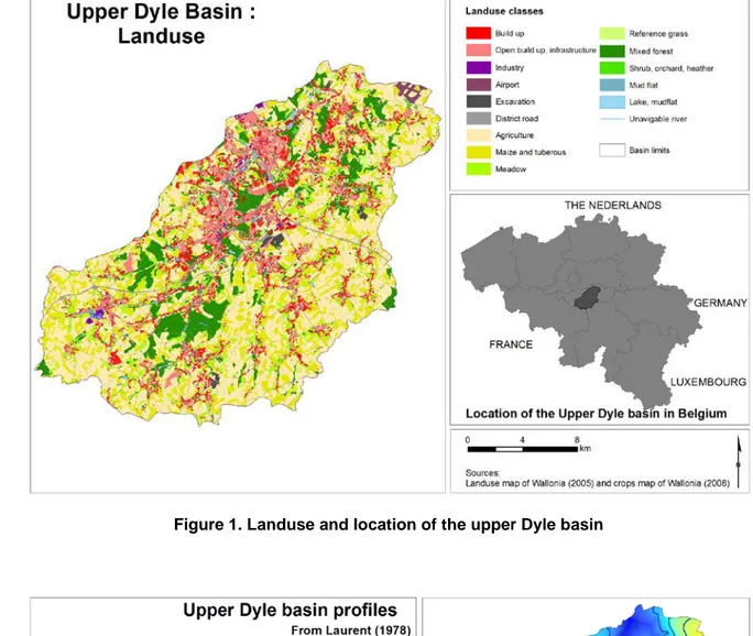
(7) 165. scale), using average climate, topographic, piezometric, land use and soil data. This approach is. 166. flexible and takes into account the spatial variation of the processes related to the recharge (Batelaan. 167. and Woldeamlak 2007). The simulated recharge can be used as an input for a groundwater model. 168. (Batelaan and De Smedt 2007; Dams et al. 2007; Jenifa Latha et al. 2010 ; Wang et al. 2010). The. 169. basin or region is considered as a regular pattern of raster cells, further subdivided in a vegetated,. 170. bare soil, open water and impervious surface fractions for which independent water balances are. 171. calculated (Batelaan and De Smedt 2007). The water balance of a cell is simply the sum of the water. 172. balances of each fractions of the cell. For more details about the methodology, see Batelaan and De. 173. Smedt (2001), Batelaan and De Smedt (2007), and Batelaan and Woldeamlak (2007).. 174 175 176. 3. Application on the upper Dyle basin 3.1. Geographical, geological, and hydrogeological context. 177. The Dyle basin is located in the central zone of Belgium (Figure 1). For this study, only the upper basin. 178. is considered, in which the Dyle stream has a length of 35 km. The upper basin is about 439 km . The. 179. elevation ranges from 35 to 175 m with an average of 122 m. Given the latitude and the proximity to. 180. the sea, the climate is maritime humid temperate characterised by average annual temperature of. 181. 10°C. 182. evapotranspiration is estimated to 550 mm/year (ibid.). More than half of the surface of the Dyle basin. 183. is covered by agriculture (57 % in 2008, Figure 1). Since agriculture constitutes one of the main source. 184. of groundwater nitrate contamination (DGARNE 2010), the Dyle basin is an interesting region for such. 185. a study. Several studies showed that concentrations of more than the norm of 50 mg/L have been. 186. observed in groundwater (Sohier et al. 2009 ; Mattern et al. 2009). 187. 2. (Walloon. Region. 2005).. Average. rainfall corresponds. to 830 mm/year. and. actual. Figure 1. Landuse and location of the upper Dyle basin in Belgium. 188 189. Geologically, nearly horizontal layers of the Cenozoic and Mesozoic eras overlie the highly fractured. 190. Paleozoic bedrock (Houthuys et al. 2011). Cenozoic formations are Paleogene clays and sands. 191. (Brussels sands), extended homogeneously. Mesozoic era is represented by Cretaceous chalks,. 192. located in the north part of the basin. Typical cross-sections show that the rivers are draining. 193. Paleogene sands, Cretaceous chalks and the Paleozoic bedrock (Figure 2). The fractured Paleozoic. 194. bedrock constitutes a low permeability basement, depending on the fracturation and nature of the. 7.

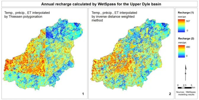
(8) 195. rocks. Two main aquifers can be highlighted, the first one in the Cretaceous chalk, the second one in. 196. the Brussels sands. These two aquifers are locally separated by a thin clay layer of low permeability. 197. as described in Dassargues and Ruthy (2001 and 2002). The hydraulic gradient of groundwater flow is. 198. very low on the interfluves and very steep close to rivers and discharge zones (Peeters 2010, Peeters. 199. et al. 2010).. 200. Figure 2. Typical geological profiles in the upper Dyle basin and piezometric map (average mid-. 201. seventies to 2007), according to Peeters (2010). 202 203. 3.2. Spatially-distributed recharge determination. 204. The recharge was calculated using the WetSpass model. This study considered two hydrological. 205. seasons, with summer ranging from April to September and winter from October to March, similarly to. 206. the study of Batelaan and De Smedt (2007). A large set of data is required to run WetSpass. The pre-. 207. processing used to create the inputs as well as the data needed are listed in Table 1. As shown in. 208. Table 1, different interpolations methods were undertaken. Consequently, ten WetSpass models. 209. resulting from the ten combinations of the meteorological data interpolations were tested. Figure 3. 210. gives an example of all raster data needed for modelling the recharge, in addition to land use data,. 211. piezometry (already shown in Figures 1 and 2) and wind speed. In Figure 3, temperature, precipitation. 212. and evapotranspiration are interpolated by the inverse distance weighted method.. 213. Table 1. Data needed and methods used to estimate WetSpass inputs. 214 215. Figure 3. Example of input raster data used for the implementation of the WetSpass model. 216. (piezometry, land use and wind excepted). 217 218. The application of the WetSpass model with the different combinations of inputs has a similar mean. 219. global annual recharge. It was found that maize and tuberous areas are the first contributors to. 220. groundwater recharge, with a mean of 363 mm/year against 270 mm/year for other diverse crops. It is. 221. interesting to note that maize and tuberous are associated with a higher charge in nutritive elements. 222. and so, a higher risk for groundwater (Batelaan and De Smedt 2007). On the contrary, urban areas. 223. correspond to low recharge zones, with a mean of 160 mm/year. The comparison of the recharge. 224. results presented in Figure 4 with literature (Meyus et al. 2004; Batelaan and De Smedt 2007; Peeters. 8.

(9) 225. 2010) showed that the WetSpass model was applied correctly and that the spatially-distributed. 226. recharge could be used as an input for the hydrogeological model.. 227. Figure 4. Annual recharge calculated by the WetSpass model. 228 229. 3.3. Numerical model. 230. The Upper Dyle basin model consists in a 3D regional model containing two layers. The model limits. 231. are the catchment boundaries. A zero flow second type boundary condition was thus prescribed,. 232. considering that there is no groundwater and not solute exchange with the neighbouring watersheds,. 233. except for a 8 km long portion where the Dyle basin gains a flux of 0.33 m³/s from the neighbouring. 234. Gette watershed (Dassargues et al. 2001). In this portion, the surface water divide does not coincide. 235. with the groundwater divide, as shown by Peeters (2010). For this portion, a third type boundary. 236. condition was prescribed, the exchanged groundwater flux being calculated based on the difference in. 237. hydraulic heads across the boundary and a first-order transfer coefficient (Figure 5). The bottom layer. 238. contains three facies: the Paleozoic basement, the Cretaceous chalks in the North and the. 239. Carboniferous limestones in the South. The upper layer is composed by the Brussels sands and the. 240. alluvial formations and is divided into seven different materials (Figure 6). A total of 11 subdomains are. 241. considered; the area being first divided into three sub-basins where baseflow rates measurements are. 242. available for calibration and then further subdivided to take into account the presence or absence of. 243. clay. Internal first type dynamic boundary conditions are prescribed between these subdomains to. 244. assume the continuity in hydraulic heads across the interface boundary. The thin clay layer locally. 245. separating the upper aquifer (Brussels sands) from the lower aquifer (Cretaceous chalks) is. 246. represented using a conductance coefficient that depends on the local thickness and hydraulic. 247. conductivity of the clay layer. Volumes extracted in pumping wells were calculated on the basis of a. 248. database. The 3D mesh is composed of 12,750 elements and 9,933 nodes.. 249. Figure 5. Internal and external boundary conditions used for the groundwater flow modelling of. 250. the upper Dyle basin. 251. Figure 6. 3D finite element mesh and zonation used for the groundwater flow modelling of the. 252. upper Dyle basin. 253. 9.

(10) 254. A solute transport model is used for simulating the spatial and temporal long term evolution of nitrates. 255. at regional scale. Therefore, short term concentration variations associated to piezometric variations. 256. are not considered to be reproduced. Consequently, a steady-state simulation can be supposed. 257. acceptable to represent average conditions for the considered period. Transient conditions are used to. 258. model nitrate transport in order to reproduce the general nitrate concentration evolution over time. 259. (Orban et al. 2010).. 260 261. The HFEMC technique has been applied in the present study for its ability to combine a classical. 262. approach, based on the calculation of the Richard’s equation, for modelling the groundwater flow, and. 263. a simplified approach, based on the mixing cell technique, to model solute transport. The relatively. 264. high level of knowledge about hydrogeological conditions in the Dyle basin allows solving the. 265. groundwater flow problem using the classical spatially-distributed groundwater flow. For the solute. 266. transport problem, solving the advection-dispersion equation at regional scale remains a huge. 267. challenge from a numerical point of view. However, considering that the main source of nitrate in the. 268. Dyle basin comes from agriculture, the nitrate pollution can be considered as diffuse and, in this. 269. particular case, the hydrodynamic dispersion in groundwater will be negligible with regards to the. 270. dispersion of the source (Duffy and Lee 1992; Orban et al. 2010). Consequently, the spatially-. 271. distributed mixing cell equation is selected as a good compromise between accuracy, robustness, and. 272. physical soundness to model nitrate transport at the regional scale (Orban et al. 2010). Without any. 273. denitrification evidences (oxic conditions clearly prevail throughout the aquifer), nitrate is assumed to. 274. be conservative in the aquifers of the Dyle basin (no degradation) (Christakos and Bogaert 1996;. 275. Mattern et al. 2009).. 276 277. Data used to implement the hydrogeological model concern primarily the geometry and the geology,. 278. the flow parameter values (hydraulic conductivity and effective porosity), the stress factors (recharge. 279. resulting from the application of the WetSpass model and pumping flow rates) and historical data. 280. concerning measured hydraulic heads, stream flow rates, and solute concentrations (DGARNE 2010).. 281 282. 3.4. Calibration of the groundwater flow model. 10.

(11) 283. The groundwater flow model was calibrated under steady-state conditions corresponding to average. 284. observations for the period 1995-2000. Observations points used for calibration consist in 21. 285. piezometric heads (figure 10) from the monitoring network in Wallonia (DGARNE 2010; Rentier et al.. 286. 2010) and three baseflow rates estimated using the VCN3 method from hydrographs measured on. 287. streams of the basin. The frequency of hydraulic head measurements was either daily, weekly or. 288. monthly and/or irregularly. Generally, the series contain at least weekly measures for the period 1995-. 289. 2000. Each observation was weighted to take into account the quality of the measurement (Hill and. 290. Tiedeman 2007), lower weights being assigned to the base flows since these ones have been. 291. calculated and not measured. The number of calibration points is rather limited given the size of the. 292. basin but there were no other data available than these given by the 21 piezometers. Calibration was. 293. performed by modifying the values of hydraulic conductivity, vertical conductance coefficients of the. 294. clay layer, and exchange coefficients between the Dyle and the Gette basin as well as between rivers. 295. and groundwater.. 296 297. The first step of the calibration process consisted in performing a sensitivity analysis using the PEST. 298. code (Doherty 2005). The PEST code calculates the composite scaled sensitivity (css), which is a. 299. measure of the sensitivity of one parameter to all observations (Hill et al. 1998; Hill and Tiedeman. 300. 2007): 1/2. ∑ND i=1(dssij )²|b cssj = � � ND. 301. where i is the considered observation, j is the considered parameter, ND is the number of. 302. observations, b is the vector containing the values of the parameters for which sensitivities are. 303. analysed and dss is the dimensionless scaled sensitivity indicating the importance of an observation. 304. on the estimation of a parameter (USGS, 2006).. 305 306. Next to the sensitivity metrics suggest by Hill and Tiedeman (2007), the sensitivity indices presented. 307. by Doherty and Hunt (2009) are worthwhile considering. The parameter identifiability value, which. 308. varies between zero and one, with zero indicating complete non-identifiability and one indicating. 309. complete identifiability, is defined as the capability of model calibration to constrain parameters used. 310. by a model (ibid.). As seen in Figure 8, the identifiable parameters are quite identical to those defined. 311. as the most sensitive using composite scaled sensitivities.. 11.

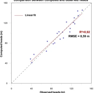
(12) 312. Figure 7. Composite scale sensitivity values of the parameters. 313. Figure 8. Parameter identifiability values. 314 315. Thanks to this estimate of the global sensitivity of each parameter, it is possible to select the. 316. parameters to be included in the calibration process. A parameter with a css value lower than 1 or. 317. lower than 1/100 of the maximum css value is considered as poorly sensitive (Hill and Tiedeman. 318. 2007). The low sensitive parameters are, in practice, given a fixed value estimated from the. 319. hydrogeological database. Consequently, one hydraulic conductivity and two exchange coefficients. 320. are fixed according to the values of the literature (Table 2). The composite scale sensitivity values are. 321. represented in Figure 7. As the recharge is calculated by WetSpass and prescribed to the. 322. groundwater flow and transport models, this parameter is not included in the optimisation process.. 323. However, the sensitivity of the recharge is calculated together with the sensitivity of the other. 324. parameters for a comparison purpose. As shown in Figure 7, hydraulic heads and discharge rates are. 325. very sensitive to the recharge which highlights the necessity of an accurate estimate of this parameter. 326. for groundwater flow and transport models.. 327 328. The remaining parameters were calibrated using the PEST code, which minimises an objective. 329. function representative of the discrepancies between observed values and their simulated equivalent: ND. S(b) = � ωi �yi − y ′ i (b)� i=1. 2. 330. with ND the number of observations, ωi the i observation weight, b the parameter, yi the observed. 331. value of the i observation and y’i the simulated value associated to the i observation (Doherty 2005).. th. th. th. 332 333 334. The resulting calibrated parameters for the steady-state calibration are listed in Table 2. Table 2. Optimized hydraulic conductivity values of the Upper Dyle basin. 335 336. Optimized hydraulic conductivities are in the same order of magnitude as those found in the literature. 337. (Dassargues and Monjoie 1993; Dassargues and Ruthy 2001; Peeters 2010). The hydraulic. 338. conductivity of Paleozoic and Precambrian bedrock is low but in the range given by Dassargues and. 339. Ruthy (2001). The chalk hydraulic conductivity is in the same range than the one given in Dassargues. 12.

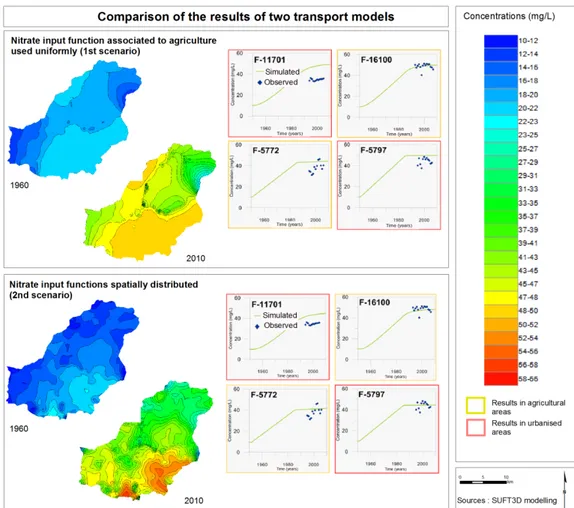
(13) 340. and Monjoie (1993). The three classes of Brussels sands have a similar hydraulic conductivity and. 341. their values are closed to the one found in Possemiers et al. (2012).. 342 343. The calibrated computed heads were compared to the measured heads (Figure 9). The RMS error is. 344. 8.6 m. This RMS error is still quite high and is certainly due to the assumptions made in the conceptual. 345. model (see discussion below). The RMS error obtained for the baseflow is 0.37 m³/s. To further. 346. compare the results, it is also interesting to refer to the piezometric map obtained by the ‘Bayesian. 347. Data Fusion’ technique (Peeters 2010) with a large number of observation points (176). The. 348. comparison shows that the model gives a good representation of the general configuration of. 349. piezometry and the influence of drainage (Figure 10). However, while groundwater flow in the Dyle. 350. catchment is highly influenced by the topography, the drainage network is not as pronounced in figure. 351. 10a and 10b. This is probably due to the use of a finite element mesh composed of relatively large. 352. elements and without any refinement along the drainage network.. 353 354. Figure 9. Comparison between observed and computed heads of the groundwater flow model. 355. of the upper Dyle basin. 356 357. Figure 10. Comparison of the piezometric maps, a) from Peeters (2010); b) obtained with the. 358. distributed recharge calculated by WetSpass, and location of observation points used in the. 359. calibration (in black). 360 361. 3.5. Implementation of the groundwater nitrate transport model. 362. The nitrate transport model was developed in transient conditions using the calibrated steady-state. 363. flow model. The simulation was performed from 1950 to 2010 following three different simple. 364. scenarios, represented in Figure 11. Constant nitrate concentrations of 0 mg/L and 10 mg/L are. 365. associated to the recharge in urbanised areas and forests respectively. A linear increase of nitrate. 366. input between 10 mg/L in 1950 and 50, 60 and 70 mg/L in 1985 is associated to infiltration from. 367. cultivated areas (oral communication, Nitrawal organism in Wallonia). After 1985, a constant nitrate. 368. input is considered. The simplified nitrate input functions are distributed spatially on the basin,. 369. according to land use, as showed in Figure 11. The application of the transport model following the. 13.

(14) 370. three scenarios shows that scenarios 2 and 3 result in a higher concentration in the south part of the. 371. basin (between 47 mg/L and 56 mg/L for scenario 2 and 52 mg/L and 66 mg/L for scenario 3 in 2010). 372. while scenario 1 results in a low concentration for the three dates.. 373. Figure 11. Spatial distribution of the nitrate concentration associated to recharge and. 374. scenarios for infiltration in cultivated areas. 375. Figure 12. Concentration in nitrate resulting for the transport model and comparison of the. 376. results with observation points. 377 378. The results presented in Figure 12 show that the simulated nitrate concentrations are closed to the. 379. observed one, either in agricultural areas or in urbanised areas. In comparison with the map published. 380. by Mattern (2009), the results of the transport model are in the same order of magnitude and the. 381. approach considered here seems satisfactory. The higher nitrate concentrations in the south-eastern. 382. part of the basin are well simulated, as well as the lower concentrations in the central zone. However,. 383. the results show an overestimation of the nitrate concentration in the south-western part of the basin.. 384 385. 4. Discussion. 386. The main objective of this paper was to demonstrate the actual feasibility of linking the WetSpass. 387. model with the SUFT3D code in order to simulate the nitrate trend at the regional scale and to. 388. illustrate it on the Upper Dyle basin. However, the proposed methodology still contains a series of. 389. limitations that are discussed here.. 390 391. The WetSpass model presents the advantage of involving most of the parameters influencing the. 392. recharge. It is user-friendly and the needed data can be derived from satellite images. Nevertheless,. 393. for several data, such as land use, we have chosen to not distinguish the seasons of the year although. 394. the WetSpass model can differentiate two seasons (summer and winter). It may present limitations. 395. since seasonal variations influence land use, especially during cultural practices. However, these. 396. possible effects are limited since WetSpass allows taking into account several parameters varying. 397. from summer to winter (vegetated area, interception percentage, bare area ...). Finally, as previously. 398. mentioned, maize and tuberous cultures can have a great influence on recharge and its spatial. 399. distribution. Considering the crops of one year cannot be representative enough for providing reliable. 14.

(15) 400. long term mean recharge. However, it has been shown that this has not a great effect on the mean. 401. annual recharge since almost 80% of the differences between recharge resulting from either 2008 or. 402. 2009 crops are in a range of 15 mm/year.. 403 404. Concerning the groundwater flow model, the RMS error obtained after the calibration process remains. 405. quite high. Several conceptual choices may be discussed considering, for example, a finer zonation of. 406. the Brussels sands, more detailed data about the distribution and the thickness and the hydraulic. 407. conductivity of the clay layer. Moreover, observed values are considered as to be compared to steady. 408. state simulated values. Additionally, the observed values are also compared with computed values at. 409. the nearest node and consequently, different values of groundwater level observed in different but. 410. very close wells can be actually compared to a unique computed value (Orban, 2008). Finally, the. 411. number of piezometers used for the calibration remains here very limited. Indeed, a higher number of. 412. piezometric data could potentially improve the model calibration.. 413 414. The spatial distribution of nitrate inputs generated interesting results. However, the transport model. 415. was here not calibrated because of the lack of distributed and temporal data. The land use spatial. 416. distribution was also considered as constant over time but it is likely that it varied between 1950 and. 417. 2010 and it will vary in the future. Another simplification concerns the stationary hydrological regime as. 418. this study focuses on long-term general nitrate trends in the aquifer that can be (in a first stage). 419. considered as weakly influenced by short-term cyclic variation of groundwater levels.. 420 421. 5. Conclusion. 422. The work presented here demonstrates the feasibility of developing an integrated water and nitrate. 423. transport model at the regional scale. The practical application of the method is shown on the case. 424. study of the Upper Dyle basin. This integrated model is based on the association of the WetSpass. 425. model (water balance model) and the SUFT3D code (groundwater flow and transport model), where. 426. the outputs of the former model in terms of recharge are used as inputs by the latter model. The. 427. groundwater flow and nitrate transport model developed with the SUFT3D and its innovative HFEMC. 428. technique is based on detailed regional hydrogeological conditions and time and space distribution of. 15.

(16) 429. nitrate in groundwater. Even if a series of simplification have been considered and discussed, results. 430. seem to be reliable and using WetSpass clearly improved the results of the groundwater flow model.. 431 432. There are several perspectives to the methodology proposed in this paper. The WetSpass model and. 433. the SUFT3D code can be used in this way for a non stationary groundwater flow instead of a steady-. 434. state model. Land use and climatic changes in the future could also be considered in the scenarios to. 435. be modelled and should result in more realistic previsions. In terms of groundwater resources. 436. management, such a work could provide further very useful information for decisions makers. Other. 437. scenarios can be included (in terms of nitrate concentrations evolution, for example) and used to. 438. forecast groundwater behaviour in response to the political decisions considered or undertaken. Such. 439. a tool is thus of major interest to support groundwater managers in charge of the implementation of. 440. regulations (for example the European Water Framework Directive) on groundwater quality with. 441. respect to diffuse contamination issues such as nitrate from agriculture.. 442 443. 6. References. 444. Amin I E, Campana M E (1996) A general lumped parameter model for the interpretation of tracer data. 445. and transit time calculation in hydrologic systems. J Hydro 179: 1-21. 446 447. Barrett M E, Charbeneau R J (1996) A parsimonious model for simulation of flow and transport in a. 448. karst aquifer, Center for Research in Water Resources, Bureau of Engineering Research, The. 449. University of Texas at Austin, Austin. 450 451. Barthel R, Jagelke J, Götzinger J, Gaiser T, Printz A (2008) Aspects of choosing appropriate concepts. 452. for modelling groundwater resources in regional integrated water resources management - Examples. 453. from the Neckar (Germany) and Ouémé catchment (Benin). Phys Chem Earth 33(1-2): 92-114. 454 455. Batelaan O, De Smedt F (2001) WetSpass: a flexible, GIS based, distributed recharge methodology. 456. for regional groundwater modelling. In: Gehrels H, Peters J, Hoeh, E, Jensen K, Leibundgut C,. 457. Griffioen J, Webb B, Zaadnoordijk WJ (eds), Impact of Human Activity on Groundwater Dynamics,. 458. 269, IAHS, Wallingford, 11-17. 16.

(17) 459 460. Batelaan O, De Smedt F (2004) Seepage, a new modflow drain package. Ground Water 42(4): 576–. 461. 588.. 462 463. Batelaan O, De Smedt F (2007) GIS-based recharge estimation by coupling surface-subsurface water. 464. balances. J Hydro 337: 337-355. 465 466. Batelaan O, Woldeamlak S T (2007) ArcView Interface for WetSpass, User Manual, Version 13-06-. 467. 2007, Vrije Universiteit Brussel (BE), Department of Hydrology and Hydraulic Engineering, 75 p.. 468 469. Brouyère S (2001) Etude et modélisation du transport et du piégeage des solutés en milieu souterrain. 470. variablement saturé (Study and modeling of solutes transport and trapping in variably saturated. 471. underground environment). PhD. University of Liège, 640p.. 472 473. Brouyère S, Carabin G, Dassargues A (2004) Climate change impacts on groundwater resources:. 474. modelled deficits in a chalky aquifer, Geer basin, Belgium. Hydrogeol J 12: 123-134. 475 476. Brouyère S, Orban P, Wildemeersh S, Couturier J, Gardin N, Dassargues A (2009) The Hybrid Finite. 477. Element Mixing Cells Method: A new flexible method for modelling mine ground water problems. Mine. 478. Water Environ 28(2): 102-114. 479 480. Brunner P, Simmons C T (2012) HydroGeoSphere: A Fully Integrated, Physically Based Hydrological. 481. Model. Ground Water 5(2): 170-176. 482 483. Campana M E, Sadler N, Ingraham N L, Jacobson R L (1997) A deuterium-calibrated compartmental. 484. model of transient flow in a regional aquifer system. Tracer Hydro: 389-396. 485 486. Carabin G, Dassargues A (1999) Modeling groundwater with ocean and river interaction. Water. 487. Resour Res 35(8): 2347-2358. 488. 17.

(18) 489. Celia M A, Bouloutas E T, Zarba R L (1990) A general mass-conservative numerical solution for the. 490. unsaturated flow equation. Water Resour Res 26(7): 1483-1496. 491 492. Christakos G, Bogaert P (1996) Spatiotemporal analysis of spring water ion processes derived from. 493. measurements at the Dyle Basin in Belgium. IEEE Transactions On Geoscience And Remote Sensing. 494. 34(3): 626–642. 495 496. Collins A L, McGonigle D F (2008) Monitoring and modelling diffuse pollution from agriculture for policy. 497. support: UK and European experience. Environ Sci & Policy 11(2): 97-101. 498 499. Dams J, Woldeamlak S T, Batelaan O (2007) Forecasting land-use change and its impact on the. 500. groundwater system of the Kleine Nete catchment, Belgium, Hydro & Earth Syst Sci Discuss 4: 4265–. 501. 4295. 502 503. Dassargues A, Brouyère S, Monjoie A, (2001) Integrated modelling of the hydrological cycle in relation. 504. to global climate change, Groundwater sub-models, Final report, SSTC-BELSPO (Belgium Federal. 505. Scientific Policy), Program Global Change - Sustainable Development. 19 p.. 506 507. Dassargues A, Monjoie A (1993) Les aquifères crayeux en Belgique (The chalky aquifers of Belgium).. 508. Hydrogéologie 2: 135-145. 509 510. Dassargues A, Radu J P, Charlier R (1988) Finite elements modelling of a large water table aquifer in. 511. transient conditions. Adv Water Res 11(2): 58-66. 512 513. Dassargues A, Ruthy I (2001) Carte hydrogéologique de Wallonie (Hydrogeological map of Walloon. 514. Region), Chastre - Gembloux, 49/5-6 1/25000, Ministry of Walloon Region, DGARNE.. 515 516. Dassargues A, Ruthy I (2002) Carte hydrogéologique de Wallonie (Hydrogeological map of Walloon. 517. Region), Chastre - Gembloux, 40/1-2 1/25000, Ministry of Walloon Region, DGARNE.. 518. 18.

(19) 519. De Vries J J, Simmer I (2002) Groundwater recharge: an overview of processes and challenges.. 520. Hydrogeol J 10: 5-17. 521 522. DGARNE (2010) Etat des nappes d’eau souterraines de la Wallonie (State of groundwater in. 523. Wallonia). In Walloon Region (Belgium), http://environnement.wallonie.be/de/eso/atlas. Cited in. 524. February 2013. 525 526. Diekkrüger B, Sondgerath D, Kersebaum K C, McVoy C W (1995) Validity of agro-ecosystem models-. 527. a comparison of different models applied to the same data set. Ecol Modell 81(13): 3-29.. 528 th. 529. Doherty J (2005) PEST – Model-Independent parameter estimation – User manual – 5 edition.. 530. Watermark Numerical Computing. 531 532. Doherty J, Hunt R J (2009) Two statistics for evaluating parameter identifiability and error reduction. J. 533. Hydro 366: 119-127. 534 535. Duffy C J, Lee D H (1992) Base flow response from non-point source contamination: spatial variability. 536. in source, structure, and initial condition. Water Resour Res 28(3): 905-914. 537 538. Goderniaux P, Brouyère S, Fowler H J, Blenkinsop S, Therrien R, Orban Ph, Dassargues A (2009). 539. Large scale surface – subsurface hydrological model to assess climate change impacts on. 540. groundwater reserves. J Hydro 373: 122-138. 541 542. Goderniaux P, Brouyere S, Blenkinsop S, Burton A, Fowler H J, Orban Ph and Dassargues A (2011). 543. Modelling climate change impacts on groundwater resources using transient stochastic climatic. 544. scenarios. Water Resour Res 47(12): 1-17. 545 546. Habils F, Rorive A (2005) Carte hydrogéologique de Wallonie (Hydrogeological map of Walloon. 547. Region), Nivelles – Genappes, 39/7-8 1/25000, Ministry of Walloon Region, DGARNE.. 548. 19.

(20) 549. Hallberg K B, Keeney D R (1993) Nitrate. In: Alley W M (ed) Regional Ground-Water quality, Van. 550. Nostrand Reinhold, New York. 551 552. Harrington G A, Walker G R, Love A J, Narayan K A (1999) A compartmental mixing-cell approach for. 553. the quantitative assessment of groundwater dynamics in the Otway Basin, South Australia. J Hydro. 554. 214: 49-63. 555 556. Harter T, Davis H, Mathews M C, Meyer, R D (2002) Shallow ground water quality on dairy farms with. 557. irrigated forage crops. J Contam Hydro 55: 287-315. 558 559. Healy R W (2010) Estimating groundwater recharge. Cambrige University Press, Cambridge. 560 561. Henriksen H J, Troldborg L, Nyegaard P, Sonnenborg T O, Refsgaard J C, Madsen B (2003). 562. Methodology for construction, calibration and validation of a national hydrologic model for Denmark. J. 563. Hydro 280: 52-71. 564 565. Hill M C, Tiedeman C R (2007) Effective Groundwater Model Calibration: With Analysis of Data,. 566. Sensitivities, Predictions, and Uncertainty. John Wiley & Sons, Inc, Hoboken. 567 568. Hill M, Colley R, Pollock D (1998) A controlled experiment in groundwater flow model calibration using. 569. nonlinear regression. Ground Water 36(3): 520-535. 570 571. Houthuys R (2011) A sedimentary model of the Brussels Sands, Eocene, Belgium. Geologica Belgica. 572. 14. 573 574. Hudak P F (2000) Regional trends in nitrate content of Texas groundwater. J Hydro 228: 37-47. 575 576. Jackson B M, Browne C A, Butler A P, Peach D, Wade A J, Wheater H S (2008) Nitrate transport in. 577. Chalk catchments: monitoring, modelling and policy implications. Environ Sci & Policy 11(2): 125-135. 578. 20.

(21) 579. Jenifa Lata C, Saravanan S, Palanichamy K (2010) A semi-distributed water balance model for. 580. Amaravathi river basin using remote sensing and GIS. Int J Geomat & Geosci 1(2): 252-263. 581 582. Johnsson H, Larsson M, Martensson K, Hoffmann M (2002) SOILNDB: a decision support tool for. 583. assessing nitrogen leaching losses from arable land. Environ Model & Softw 17(6): 505-517. 584 585. Jury W A (1982) Simulation of solute transport using a transfer function model. Water Resour Res. 586. 18(2): 363-368. 587 588. Laurent E (1978) Monographie du bassin de la Dyle (Dyle Basin monograph), Ministry of Public Health. 589. and Environment, 302 p.. 590 591. Ledoux E, Gomez E, Monget J M, Viavattene C, Viennot P, Ducharne A, Benoit M, Mignolet C, Schott. 592. C Mary B (2007) Agriculture and groundwater nitrate contamination in the Seine basin. The STICS-. 593. MODCOU modelling chain. Sci Total Environ 375: 33-47. 594 595. Maloszewski P, Zuber A (1982) Determining the turnover time of groundwater systems with the aid of. 596. environmental tracers. 1. Models and their applicability. J Hydro 57: 207-231. 597 598. Mattern S (2009) Mapping and source identification of groundwater pollution by nitrate. Theory and. 599. application to the Brusselian sand groundwater body. PhD. Catholic University of Louvain, 236p.. 600 601. Mattern S, Fasbender D, Vanclooster M (2009) Discriminating sources of nitrate pollution in an. 602. unconfined sandy aquifer. J Hydro 376: 275-284. 603 604. Mitchell R J, Scott Babcock R, Gelinas S, Nanus L, Stasney D E (2003) Nitrate distributions and. 605. source identification in the Abbotsford-Sumas aquifer, Northwester Washington state. J Environ Qual. 606. 32: 789-800. 607. 21.

(22) 608. Mohamed M A A, Terao H, Suzuki R, Babiker I S, Ohta K, Kaori K, Kato K (2003) Natural. 609. denitrification in the Kakamigahara ground water basin, Gifu prefecture, central Japan. Sci Total. 610. Environ 307: 191-201. 611 612. Navarre A, Lecomte P, Martin H (1976) Analyse des tendances de données hydrochimiques du bassin. 613. de la Dyle en amont d'Archennes. Annales de la Société Géologique de Belgique 99: 299-313. 614 615. Orban Ph (2008) Solute transport modeling at the groundwater body scale : nitrates trends. 616. assessment in the Geer basin (Belgium). PhD. University of Liège, 207p.. 617 618. Orban Ph, Brouyère S, Battle-Aguilar J, Couturier J, Goderniaux P, Leroy M, Malozewski P,. 619. Dassargues A (2010) Regional transport modelling for nitrate trend assessment and forecasting in a. 620. chalk aquifer. J Contam Hydro 118: 79-93. 621 622. Orban Ph, Brouyère S, Wildemeersh S, Couturier J, Dassargues A (2008) The hydrid Finite-Element. 623. Mixing-Cell method : a new flexible method for large scale groundwater modelling, CMWR XVII -. 624. Computational Methods in Water Resources. San Francisco: USA, July 2008.. 625 626. Oren O, Yechieli Y, Böhlke J K, Dody A (2004) Contamination of groundwater under cultivated fields in. 627. a arid environment, central Arava Valley, Israel. J Hydro 290: 312-328.. 628 629. Peeters L (2010) Groundwater and geochemical modelling of the unconfined Brussels aquifer,. 630. Belgium. PhD. Catholic University of Leuven, 232p.. 631 632. Pineros Garcet J, Ordonez A, Roosen J, Vanclooster M (2006) Metamodelling: theory, concepts and. 633. application to nitrate leaching modelling, Ecological Modelling 193: 629-644. 634 635. Possemiers M, Huysmans M, Peeters L, Batelaan O, Dassargues A. (2012) Relationship between. 636. sedimentary features and permeability at different scales in the Brussels Sands. Geologica Belgica. 637. 15(3): 156-164. 22.

(23) 638 639. Meyus Y, Woldeamlak S T, Batelaan O, De Smedt F (2004) Opbouw van een Vlaams. 640. Grondwatervoedingsmodel: Eindrapport (Structure of a Flemish Groundwater Model: Final Report),. 641. Technical Report 81p., AMINAL, afdeling Water.. 642 643. Peeters L, Bação F, Lobo V, Dassargues A (2007) Exploratory data analysis and clustering of. 644. multivariate spatial hydrogeological data by means of GEO3DSOM, a variant of Kohonen's Self-. 645. Organizing Map. Hydro & Earth Syst Sci 11: 1309-1321. 646 647. Peeters L, Fasbender D, Batelaan O, Dassargues A (2010) Bayesian Data Fusion for water table. 648. interpolation: incorporating a hydrogeological conceptual model in kriging. Water Resour Res 46 (8):. 649. W08532.. 650 651. Rentier C, Delloye F, Brouyère S, Dassargues A (2006) A framework for an optimised groundwater. 652. monitoring network and aggregated indicators. Environ Geol 50(2): 194-201. 653 654. Rozos E, Koutsoyiannis D (2006) A multicell karstic aquifer model with alternative flow equations. J. 655. Hydro 325: 340-355. 656 657. Scanlon B R, Healy R W, Cook P G (2002) Choosing appropriate techniques for quantifying. 658. groundwater recharge. Hydrogeol J 10: 18-39. 659 660. Skaggs T H, Kabala Z J, Jury W A (1998) Deconvolution of a nonparametric transfer function for. 661. solute transport in soils. J Hydro 207: 170-178. 662 663. Sohier C, Degré A, Dautrebande S (2009) From root zone modelling to regional forecasting of nitrate. 664. concentration in recharge flows – The case of the Walloon Region (Belgium). J Hydro 369: 350-359. 665. 23.

(24) 666. Sophocleous M, Koelliker J K, Govindaraju R S, Birdie T, Ramireddygari S R Perkins S P (1999). 667. Integrated numerical modeling for basin-wide water management: The case of the Rattlesnake Creek. 668. basin in south-central Kansas. J Hydro 214: 179-196. 669 670. Stewart I T, Loague K (1999) A type transfer function approach for regional-scale pesticide leaching. 671. assessments. J Environ Qual 28(2): 378-387. 672 673. Sutton M, Howard C, Erisman J W, Billen G, Bleeker A, Grennfelt P, van Grinsven H, Grizzetti B (ed). 674. (2011). The European Nitrogen Assessment: sources, effects and policy perspectives. Cambridge. 675. University Press. Cambridge. 676 677. Therrien R, Sudicky E A (1996) Three-dimensional analysis of variably-saturated flow and solute. 678. transport in discretely-fractured porous media. J Contam Hydro 23(1-2): 1-44. 679 680. Therrien R, Sudicky E, McLaren R, Panday S (2005) HydroGeoSphere – A three-dimensinoal. 681. numerical model describing fully-integrated subsurface and surface flow and solute transport. Manual,. 682. Groundwater Simulations Group. 683 684. Thorburn P J, Biggs J S, Weier K L, Keating B A (2003) Nitrate in ground waters of intensive. 685. agricultural areas in coastal Northeastern Australia. Agriculture. Ecosyst & Environ 94: 49-58. 686 687. USGS (2009) Methods for estimating groundwater recharge in humid regions.. 688. http://water.usgs.gov/ogw/gwrp/methods/. Cited in February 2013. 689 690. Visser A, Dubus I, Broers H P, Brouyere S, Korcz M, Orban Ph, Goderniaux P, Batlle-Aguilar J,. 691. Surdyk N, Amraoui N, Job H, Pinault J L, Bierkens M (2009) Comparison of methods for the detection. 692. and extrapolation of trends in groundwater quality. J Environ Monit 11: 2030-2043. 693 694. Walloon Region (2005) Etat des lieux des sous-bassins hydrographiques, Tome 1 : Etat des lieux.. 695. Sous-bassin Dyle-Gette. Description générale des caractéristiques du sous-bassin (Inventory of. 24.

(25) 696. subwatershed, Volume 1: Inventory. Dyle-Gette subwatershed. General description of the. 697. subwatershed characteristics), In Walloon Region.. 698. http://environnement.wallonie.be/directive_eau/edl_ssb/dg/Dg1.pdf. Cited in February 2013.. 699 700. Wang Y, Lei X, Liao W, Jiang Y, Huang X, Liu J, Song X, Wang (2012) Monthly spatial distributed. 701. water resources assessment: a case study. Comput & Geosci 45: 319-330. 702 703. Wick K, Heumesser C, Schmid E (2012) Groundwater nitrate contamination: Factors and indicators. J. 704. Environ Manag 111: 178-186. 705 706. Wildemeersch S, Brouyère S, Orban Ph, Couturier J, Dingelstadt C, Veschkens M, Dassargues A. 707. (2010) Application of the Hybrid Finite Element Mixing Cell method to an abandoned coalfield in. 708. Belgium. J Hydro 392(3-4): 188-200. 709 710. Yi M J, Lee K K (2004) Transfer function-noise modelling of irregularly observed groundwater heads. 711. using precipitation data. J Hydro 288: 272-287. 25.

(26) 1. 2 3. Figure 1. Landuse and location of the upper Dyle basin. 4. 5 6. Figure 2. Typical profiles in the upper Dyle basin. 1.

(27) 7 8. Figure 3. Example of input raster data of the WetSpass model. 2.

(28) 9 10. Figure 4. Annual recharge calculated by the WetSpass model for two combinations of inputs. 11 12. Figure 5. 3D finite element mesh and zonation used for the groundwater modelling. 3.

(29) 2nd type external boundary condition (recharge). No-flow external boundary condition. 1st type internal boundary condition. 3rd type external boundary condition (exchange) 3rd type internal boundary condition 3rd type external boundary condition (river). 13 14. Figure 6. Internal and external boundary conditions. 15 Comparison between computed and observed heads. Computed heads (m). Linear fit. 16 17. Observed heads (m). Figure 7. Comparison between observed and computed heads. 4.

(30) 18 19. Figure 8. Comparison of the piezometric maps, a) of Peeters (2010) ; b) obtained with an. 20. uniform recharge ; c) obtained with the distributed recharge calculated by WetSpass. 21. 22 23. Figure 9. Spatial distribution of the nitrate concentration associated to recharge. 24. 5.

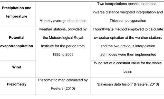
(31) 25 26. Figure 10. Comparison between the results of two transport models implemented with either a. 27. spatial distribution of nitrate input or a uniform of nitrate inputs. 28 29 30 31. Table 1. Data needed and methods used to estimate inputs Wetspass input. Data needed. Topography and. DEM provided by the Belgian. slopes. National Geographic Institute. Method used to estimate input Resampling using the nearest neighbour technique to obtain a 10 m resolution, slopes calculation. Soil map of Wallonia (2007), Pedology. Classification to fit the USDA classification USDA texture triangle (2012) Landuse map (2005) and. Classification into 20 final classes used by. crops map (2008) of Wallonia. WetSpass. Landuse. 6.

(32) Two interpolations techniques tested : Precipitation and inverse distance weighted interpolation and temperature Monthly average data in nine. Thiessen polygonation. weather stations, provided by. Thornthwaite method employed to calculate. Potential. the Meteorological Royal. evapotranspiration at the weather stations. evapotranspiration. Institute for the period from. and the two previous interpolation. 1995 to 2005. techniques were then implemented Wind set at a constant value for the whole. Wind basin Piezometric map calculated by Piezometry. “Bayesian data fusion” (Peeters, 2010) Peeters (2010). 32 33. Table 2. Optimized hydraulic conductivity values of the upper Dyle basin Parameter. Hydraulic conductivity (m/s) -06. (optimised). -05. (optimised). -03. (optimised). -04. (optimised). -04. (optimised). -05. (optimised). -07. (fixed). -04. (optimised). -04. (optimised). -02. (fixed). -08. (optimised, mean). -03. (fixed). -10. (fixed). -03. (fixed). k1 - Basement. 4.2 × 10. k2 - Chalk. 8.1 × 10. k3 - Limesotne. 5.0 × 10. k4 – Quartzitic sands. 2.0 × 10. k5 - Clay/Alluvions. 2.2 × 10. k6 - Basement/Alluvions. 1.4 × 10. k7 – Basement/Sand/Alluvions. 5.0 × 10. k8 - Sand 2. 1.3 × 10. k9 – Sand 1. 5.8 × 10. k10 – Calcareous fine sand. 1.0 × 10. Exchange coeff. between groundwater and surface water 9.0 × 10 Exchange coeff. between Dyle and Gette basin. 1.0 × 10. Vertical exchange coeff., with clay. 1.1 × 10. Vertical exchange coeff., without clay. 1.0 × 10. 34 35. 7.

(33)