HAL Id: hal-01868227
https://hal.archives-ouvertes.fr/hal-01868227
Submitted on 5 Sep 2018
HAL is a multi-disciplinary open access
archive for the deposit and dissemination of
sci-entific research documents, whether they are
pub-lished or not. The documents may come from
teaching and research institutions in France or
abroad, or from public or private research centers.
L’archive ouverte pluridisciplinaire HAL, est
destinée au dépôt et à la diffusion de documents
scientifiques de niveau recherche, publiés ou non,
émanant des établissements d’enseignement et de
recherche français ou étrangers, des laboratoires
publics ou privés.
Combining Model Learning and Data Analysis to
Generate Models of Component-based Systems
Sébastien Salva, Elliott Blot, Patrice Laurencot
To cite this version:
Sébastien Salva, Elliott Blot, Patrice Laurencot. Combining Model Learning and Data Analysis to
Generate Models of Component-based Systems. Testing Software and Systems - 30th 6.1 International
Conference, ICTSS, Oct 2018, Cadiz„ Spain. �hal-01868227�
Combining Model Learning and Data Analysis to
Generate Models of Component-based Systems
?S´ebastien Salva1, Elliott Blot1, and Patrice Laurencot1
LIMOS CNRS UMR 6158, Clermont Auvergne University, [email protected], [email protected], [email protected]
Abstract. Finding bugs in systems without model is well-known to be challenging and costly. But, most of today’s developers think that writ-ing models is also a hard and error-prone task. In this context, this paper addresses the problem of learning a model, from a component-based system, which captures and separates the behaviours of compo-nents and encodes their synchronisations. We present a passive model learning method called COnfECt to infer such models from execution traces in which no information is provided to identify components. We describe the two main steps of COnfECt in this paper and show some preliminary experimentations on real systems.
Keywords: Model learning; Passive learning; Reverse engineering; Component-based systems.
1
Introduction
Software testing aims at assessing the quality of the features offered by a system in terms of conformance, security, performance, etc., to discover and correct its defects. Nowadays, testing is essentially performed by means of test cases written by hand, which is often a long, difficult and error-prone task. To make this task easier, model learning approaches have proven to be valuable for recovering models that can be exploited by many software engineering stages, e.g. testing. Although the generation of behavioural models has been greatly studied, lit-tle attention has been given to the learning of models from component-based systems. Yet, most of the systems being currently developed are made up of reusable features or communicating components that interact together. These observations motivate this work, which adresses the challenge of how to learn a model from its traces, in such a way that the model captures the behaviour of every component of the System Under Learning (SUL) and their synchronisa-tions.
For this purpose, we designed the method COnfECt (COrrelate Extract Com-pose) for learning models of component-based systems. Its main originality is that it does not require any preliminary identification information about com-ponents. COnfECt learns a system of LTSs (Labelled Transition Systems) from
?
Research supported by the VASOC Project and the French Region Auvergne-Rhˆ one-Alpes (https://vasoc.limos.fr/)
traces (passive learning), which captures the behaviours of every component by a LTS and shows how they are synchronised together. COnfECt is composed of two main steps called Trace Analysis & Extraction and LTS synchronisation which are going to be developped in this paper.
Paper organisation: Section 2 introduces the two steps of the COnfECt approach. The next section summarises the results of a preliminary evaluation on an IOT (Internet Of Things) device. Finally we conclude in Section 4.
2
The COnfECt Approach
Beforehand, we recall that the LTS model, we use in this paper, is defined in terms of states and transitions labelled by actions, taken from a general action setL, which expresses what happens (a more complete definition can be found in [2]). We also define special actions of the form call Ci and return Ci to model
component calls with Ci referring to a LTS. Actions of the form call Ci and
return Ci synchronise pairs of LTSs as described in[1]. The execution of Ci
starts with the label call Ci and ends when the transition return Ci is fired.
2.1 Overview of COnfECt
The COnfECt method aims to infer a system of LTSs SC from the traces of SUL, in such a way that SC captures the behaviours of the SUL components and their synchronisations. COnfECt initially requires the set of traces of SUL, denoted T races(SUL), to analyse the system behaviours and identify components. We suppose that each component can be identified by its behaviour, materialised by action sequences. And the more traces, the more correct the component detection will be. SUL can be indeterministic, uncontrollable or can have cycles among its internal states. However, we assume SUL and T races(SUL) obey certain restrictions. We consider that SUL has components whose observable behaviours are not carried out in parallel. One component is executed at a time from its initial state to one of its final states. Furthermore, we consider that traces are collected in a synchronous manner (by means of synchronous communications) to avoid the interleaving of actions. Traces can be collected by means of monitoring tools or extracted from log files. We assume that T races(SUL) does not include actions expressing the calls of components.
Furthermore, although this task is costly and important, we do not focus this work on the trace formatting, hence, we assume having a mapper, which is a tool often required in model learning to transform raw execution traces into higher level representations.
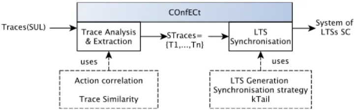
COnfECt has two main successive steps illustrated in Figure 1. The first step, called Trace Analysis & Extraction tries to detect components in T races(SUL), which is partitioned into a set of trace sets called ST races. Each trace set of ST races captures some behaviours of one component. The second step, called LTS Synchronisation, takes the set ST races and starts with the generation of one LTS for each trace set of ST races. This step also proposes different synchro-nisation strategies to generate a system of LTSs SC, before merging equivalent states with kTail.
Fig. 1: The COnfECt approach overview
2.2 Trace Analysis & Extraction
The aim of this step is to identify the different components in the traces of T races(SUL). The algorithm, which is given in [2] is divided into three pro-cedures. The first one, Inspect analyses the traces and segments them in sub-sequences. We define a Correlation Coefficient to evaluate the correlation of suc-cessive actions in T races(SUL), i.e. the degree to which sucsuc-cessive actions are associated with regard to T races(SUL). We define the Correlation coefficient between two actions by means of a utility function, which involves a weighting process for representing user priorities and preferences. We have chosen the tech-nique Simple Additive Weighting (SAW) [3], which allows the interpretation of these preferences with weights. This factor must take a value between 0 and 1, and needs to be appraised, depending of the context.
From this Correlation coefficient, we define a relation to express the notion of strong correlation. We say that strong-corr(σ1) holds when σ1 has successive
actions that strongly correlate. Besides, we compare two sequences with the re-lation σ1 mismatch σ2, which holds when the last event of σ1does not correlate
strongly with the first one of σ2.
The second procedure Extract whose algorithm is also given in [2] creates recursively different sequences to express component calls. It takes every trace σ, transforms it and stores the new trace into a set Tj, by the means of the
coefficient correlation.
(a) Procedure Extract steps (b) Component call Fig. 2: Sequence extraction example
Example 1. Let us illustrate the procedure Extract with the example of Figure 2a. The procedure takes as input a trace initially segmented into 4 sub-sequences
by the correlation coefficient. A) We start at σ1and suppose that no other
sub-sequence is strongly correlated with σ1. The sequence σ2σ3σ4is hence extracted
and replaced by the actions call C2 return C2, which model the call of a compo-nent C2. The procedure is recursively called with Extract(σ0= σ2σ3σ4, T2). B)
We now suppose σ2σ4 strongly correlate, thus σ3 is extracted and the sequence
σ0 becomes σ0= σ2.call C3 return C3.σ4. The extracted sequence σ3cannot be
segmented. It is surrounded with the actions call C3 and return C3 to prepare the LTS synchronisation and to express that C3 is called by another component. The resulting sequence is added to the set T3. As σ0 is completely covered, σ0 is
surrounded with the actions call C2 and return C2 and added to the new trace set T2. At the end of this process, we have recovered the hierarchical component
call depicted in Figure 2b and we get three trace sets.
The set T1, which holds the modified traces of the initial traces set T races(SUL),
may include traces resulting from several components. We call the third proce-dure Separate for trying to partition T1, to build the set ST races such that a trace set T of ST races is produced by one component. For that, we evaluate the trace similarity with regard to the actions shared between pairs of traces. Among the different available coefficients, we chose the Overlap coefficient be-cause the action sets used by two traces may have different sizes. Then a clus-tering technique is used to get the equivalence classes. The procedure Separate is implemented with a Similarity threshold here.
2.3 LTS Synchronisation
The previous step of COnfECt has segmented, extracted and modified the traces of T races(SUL) in such a way that each traces set contains the behaviour of only one component. We generate a LTS from every traces set, where each trace rep-resent a path of a tree-like LTS. These LTSs include actions of the form call Ci
and return Ci. These actions were added in the previous step to prepare the
synchronisation of components with LTSs. We proposes different synchronisa-tion strategies, which provide systems of LTSs with different levels of generalisa-tion. The strict synchronisation limits over-generalisation, and used only kTail to merge equivalent states. The weak synchronisation aims at reducing the num-ber of models and allows repetitive components calls, its uses a LTS similary coefficient to merge models by means of a clustering technique. The strong syn-chronisation generate callable-complete LTSs, i.e., the LTS can call any other LTS of the system from any states.
Example 2. Let us illustrate this step with the set ST races of Figure 3. The traces T 1 to T 4 are obtained from the step Trace Analysis & Extraction on a trace collected from a real smart thermostat device at the HTTP level. This trace, composed of 16 actions, was formatted to keep the Urls and some data, e.g., the temperature.
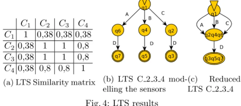
We choose to apply the Weak synchronization strategy. A similarity matrix is computed by means of the LTS Similarity coefficient. Figure 4a shows the matrix obtained with the four LTSs of our example. We can observe that two
STraces = {
T1 {/devices call_C2 return_C2 Response(status:=200,data:=[1]) call_C3 return_C3 /devices Response(status:=200,data:=[1]) /hardware Response(status:=200,data:=[2]) /config call_C4 return\_C4 Response(status:=200,data:=[2]) /tools Response(status:=200,data:=[3])} T2 {call_C2 /json.htm(idx:=115,svalue:=15.00)=A Response(status:=200)=D return_C2} T3 {call_C3 /json.htm(idx:=115,svalue:=16.00)=B Response(status:=200)=D return_C3} T4 {call_C4 /json.htm(idx:=0,switchcmd:=On)=C Response(status:=200)=D return_C4} }
Fig. 3: Example of formatted trace segmented into 4 trace sets.
classes of similar LTSs emerge in this matrix: (C1) and (C2, C3, C4). A clustering
technique is used to generate these classes. The LTSs of each cluster are then joined by means of a disjoint union.
C1 C2 C3 C4
C1 1 0,38 0,38 0,38
C20,38 1 1 0,8
C30,38 1 1 0,8
C40,38 0,8 0,8 1
(a) LTS Similarity matrix (b) LTS C 2 3 4 mod-elling the sensors
(c) Reduced LTS C 2 3 4 Fig. 4: LTS results
From the trace sets of Figure 3, we obtain the two LTS clusters: (C1) and
(C2,C3,C4), the first one expressing the behaviour of the Web interface, and
the other one, the component that sends data. Figure 4b depicts the LTS C234
derived from the second cluster. The LTS C234holds two equivalent state classes
(q2, q4, q6) and (q3, q5, q7). kTail merges them and returns the LTS of Figure 4c.
3
Preliminary Evaluation
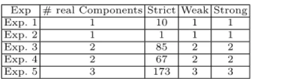
We have implemented COnfECt in a prototype tool on which we conducted several experiments. We initially collected traces from an IOT device, a smart connected thermostat. It integrates 3 components providing HTTP traces. Sev-eral experiences have been performed, only five of them are provided in Table 1 and 2 : exp 1 and 2, traces of only one component is recovered, exp 3 and 4, traces of 2 components, and the last one with all the components.
Firstly, we evaluated the capability of COnfECt to recover the correct number of components, and then we compared the number of states and transitions with kTail. The tool, the trace sets and results are available here 1. In Table 1, for
exp. 1 to 5, the number of LTSs is equal to the number of real components with the Weak and Strong strategies, but not with the Strict strategy. This strategy segments traces, which are lifted to the level of LTS, but these are not merged.
Table 2 gives the number of states and transitions of all the LTSs generated by COnfECt in Exp. 1 to 5. We also provide the number of states and transitions of these LTSs after removing the transitions labelled by the synchronisation actions in the last three columns. For comparison purposes, we applied kTail
1
Exp # real Components Strict Weak Strong Exp. 1 1 10 1 1 Exp. 2 1 1 1 1 Exp. 3 2 85 2 2 Exp. 4 2 67 2 2 Exp. 5 3 173 3 3
Table 1: Number of components detected by COnfECt.
Exp. kTail Strict Weak Strong Strict+hide Weak+hide Strong+hide #states #trans #states #trans #states #trans #states #trans #states #trans #states #trans #states #trans
Exp 1 40 66 152 169 46 78 60 150 120 137 39 70 36 67
Exp 2 6 8 6 8 6 8 6 8 6 8 6 8 6 8
Exp 3 60 115 731 691 104 188 72 183 399 359 71 124 36 85
Exp 4 22 47 496 470 41 81 25 57 236 210 24 55 10 23
Exp 5 85 175 1307 1185 158 286 82 197 627 505 96 169 36 87
Table 2: Size of the LTSs obtained with kTail and the three strategies of COn-fECt. The label ”hide” refers to the removal of the LTS transitions labelled by synchronisation actions.
on the same trace sets. As expected, we obtain bigger LTSs with COnfECt than the ones achieved by kTail (excepted with Exp. 2 since there is no trace segmentation). This result comes from the functioning of our method since the LTSs are completed with transitions labelled by synchronisation actions.
The transitions labelled by synchronisation actions help interpret the com-ponents combination and are required to compose LTSs, but are not relevant if one want to focus on the component behaviours only. If we remove them, the models achieved by COnfECt become more concise than those obtained with kTail.
4
Conclusion
We have introduced COnfECt, a passive model learning method that gener-ates systems of LTSs from execution traces. A system of LTSs captures the behaviours of components and their synchronisations. COnfECt detects com-ponent behaviours by analysing traces with a Correlation coefficient and Sim-ilarity coefficients. It proposes different LTS synchronisation strategies, which help manage the model generalisation. With this hierarchic component organi-sation, we believe it offers better readability and comprehensibility than classical learned models, and consequently can be easily used for testing. In future work, we plan to perform more evaluations of COnfECt on several kinds of systems. We also plan to use the models for security testing.
References
1. van der Bijl, M., Rensink, A., Tretmans, J.: Compositional testing with ioco. In: Petrenko, A., Ulrich, A. (eds.) Formal Approaches to Software Testing. pp. 86–100. Springer Berlin Heidelberg, Berlin, Heidelberg (2004)
2. Salva, S., Blot, E., Lauren¸cot, P.: Combining Model Learning and Data Analysis to Generate Models of Component-based Systems. Limos research report (May 2018), http://sebastien.salva.free.fr/RR-18-05.pdf
3. Yoon, K.P., Hwang, C.L.: Multiple attribute decision making: An introduction (quantitative applications in the social sciences) (1995)