Bayesian estimation of correlation matrices: Application to the Multivariate GARCH model

(1)

Bayesian estimation of correlation matrices:

Application to the Multivariate GARCH model

By

Pierre Evariste NGUIMKEU NGUEDIA

To fulfill the degree of Master in Economics

Advisor: Prof. William McCAUSLAND

Department of Economics University of Montreal

(2)

Abstract*

The correlation matrix (R) plays an important role in many statistical and financial models. Unfortunately, sampling the correlation matrix can be problematic because of its positive definite constraint and its diagonal elements fixed at 1. In this work, we use the geometric properties of the correlation concept together with a Metropolis random-walk algorithm to estimate the constant correlation matrix in the Multivariate GARCH models as well as its parameters. The theory of the MH algorithm used to estimate the parameters of the model and sufficient conditions to implement it are shown in details. We also give an overview of the methodology used to sample the correlation matrix. Using these algorithms, we draw all elements of R by simulating a common prior distribution for all correlations and accepting posterior draws based on a Random Walk Metropolis-Hastings acceptance probability. The algorithm is applied using a multivariate GARCH model on financial time series from three daily stock returns from the energy sector. We then provide some interesting posterior distributions illustration and model parameters estimates.

Key words: Correlation matrix, Bayesian inference, GARCH,

Metropolis-Hastings.

(3)

List of figures

Figure 1: Returns of Exxon Mobil (XOM) and Total (TOT) from 8/1/2006 to 7/31/2008 10 Figure 2: Returns of Chevron (CVX) and Total (TOT) from 8/1/2006 to 7/31/2008 ... 10 Figure 3: Returns of Chevron (CVX) and Exxon Mobil (XOM) from 8/1/2006 to 7/31/2008 ... 10 Figure 4: Histograms and draws of the posterior sample of the GARCH parameters for XOM (N=10000) ... 12 Figure 5: Histograms and draws of the posterior sample of the GARCH parameters for TOT (M=10000) ... 13 Figure 6: Histograms and draws of the posterior sample of the GARCH parameters for CVX (N=10000) ... 15 Figure 7: Plots of histograms and draws of the correlation matrix elements ... 17

List of tables

Table 1: Parameters estimates for XOM (M=10000) ... 12 Table 2: Parameters estimates for TOT (M=10000) ... 14 Table 3: Parameters estimates for CVX (M=10000) ... 15 Table 5: Posterior Correlation Matrix (means and standard deviations) of the M-GARCH model obtained with M=10000 accepted draws ... 18

(5)

I. INTRODUCTION

The correlation matrix (R) is directly involved in a variety of financial models. Indeed, the importance of risk and uncertainty in modern economic theory and the statistical properties of asset returns have necessitated the development of new econometric time series techniques that allow for modeling variances and correlations.

The Generalize autoregressive conditional heteroscedastic (GARCH) model (Bollerslev et al. (1992)) has been very popular in modeling the volatility of financial time series. The extension of univariate GARCH-type models to a multivariate framework and the estimation of correlations between asset returns are important for asset pricing, risk management and portfolio analysis; see, for example, Gourieroux (1997).

Correlations may also be useful to give substantive information about firms’ behavior. For example, for companies engaged in strategies where they expand and/or change the products and services that they offer or for hybrid companies that may not fit to a specific industrial classification (for example, energy or finance), it may be of interest to determine whether their stock behavior is correlated with that of a particular class of companies (see Liechty, Liechty and Muller (2004)).

Sampling the correlation matrix in such models is thus necessary but can be problematic due to three major problems: The larger number of parameters to be estimated, the difficulty of the estimation due to the positive definiteness restrictions and the fixed diagonal elements of the correlation matrix. Due to these difficulties, several methods of simulation have been proposed:

Barnard, McCulloch and Meng (2000) suggested using the Griddy Gibbs sampler to draw the components of a correlation matrix one at a time in the context of a hierarchical shrinkage model for the marginal variances of a covariance matrix.

(6)

Although the Griddy Gibbs sampler is simple to implement, it is not computationally efficient.

Liechty, Liechty and Muller (2004) provide another approach to simulate all the components of the correlation matrix one by one through introduction of a latent variable. Other similar approaches have been discussed in Bowen and Lombrano (1998), Daniels and Kass (1999).

Belin (2004) proposed a parameter-extended Metropolis-Hastings algorithm (PX-MH) for sampling R in Bayesian models with correlated latent variables. The seminal idea in their method is that instead of a marginal prior for R, they specified a joint prior for R and D (unidentified marginal variances) derived from some inverse Wishart distribution. Then sampling (R;D) jointly was accomplished through a Metropolis Hastings algorithm.

Liu and Daniels (2006) propose a two-stage parameter expanded re-parameterization and Metropolis-Hastings (PX-RPMH) algorithm for simulating a correlation matrix from its conditional distribution. In stage 1, R can be transformed into a less constrained covariance matrix, say Σ = DRD, such that the posterior distribution of Σ is an inverse Wishart distribution. In the second stage, simulating R in the original model is equivalent to first simulating Σ from the inverse Wishart distribution in the new model, and then translating it back to R through the reduction function (R=D-1ΣD-1) and accepting it based on a Metropolis-Hastings (M-H)

acceptance probability.

In this study, we use the geometric properties of the linear correlation concept together with a Metropolis random-walk algorithm to estimate the correlation matrix in the Multivariate GARCH models as well as its parameters. The common correlation approach (Liechty and Liechty 2004) we use here assumes a common prior for all correlations, with the additional restriction that the correlation matrix is positive definite. The former condition is obtained by simulating a common prior distribution for all correlations. The latter condition is straightforward as it follows

(7)

from the Cholesky product of unit vector of the matrice rows computed during the algorithm.

The rest of the work is organized as follows. In Section 2, we review Multivariate GARCH (M-GARCH) models and techniques to sample from their respective posterior distributions. In Section 3, we present the geometric approach for sampling a correlation matrix. This algorithm is derived for M-GARCH models with a common correlation prior. We also present a Metropolis-Hasting algorithm used to sample the model parameters. Their implementation and properties are explained in detail. A simulation study and application to real data from three daily stock returns from three companies of the energy sector is reported on in Section 4. Finally, we summarize our conclusions.

II. THE MULTIVARIATE GARCH MODEL

We wish to conduct Bayesian inference on a regression model with GARCH errors. For simplicity we use the GARCH (1, 1) model which is quite representative of GARCH models used in finance.

II . 1 . Model specification and notations

We consider a multivariate financial time series observations yt t 1,..,T

with K elements each, so that ' 1

( ,..., )

t t Kt

y y y and we assume that the observations are of zero mean. Let H_t denote the time-varying conditional covariance matrix of

t y , ie:

1

( _t _t ) _t

Var y I H

Where I_t ₁ is the -field generated by all the available information up to

time t 1, and H_t is almost surely positive definite for all t. The variance elements

of H_t are 2

it it

h , for i 1,...,K , and the covariance elements are hijt ijt, where

(8)

Following Bollerslev (1990), the full conditional covariance matrix H_t may

be partitioned as:

t t t

H S RS

where S_t denotes the KxKstochastic diagonal matrix with elements

1t,..., Kt, and R is a KxK time-invariant matrix with elements rij.

Define 1

t S yt t. Thus, t is the standardize residual, and is assumed to be

serially independently distributed with mean zero and variance matrixR.

To specify the conditional variance of y_t, a univariate GARCH (1,1) model

for the marginal variances h_it (H_{t ii}) can be defined as :

2 , 1 , 1 (0,1) it it it it it i i i t i i t y h N h h 

Researcher adopting the vech-diagonal form typically assume that the above equation also apply to the conditional covariance terms h_ijt (H_{t ij}) , in which h_it is

replaced by hijt and

2

it by it jt.

In our framework, we model multivariate time series data by assuming a univariate GARCH (1,1) model for marginal variances as defined above, and completing the model with a structured prior for correlation matrix, using the prior models proposed in the following paragraphs.

II . 2 . Prior specification and posterior analysis

Prior specification

In order to estimate the posterior distribution, a prior distribution ( , )R of the unknown parameters and R needs to be specified. For Bayesian inference, it

(9)

is common to specify independent priors for andR. In absence of prior

knowledge, it is also desirable to have uninformative priors on the parameters we are estimating.

Prior specification on _i, _i and _i

Let _i denotes the parameter vector ( _i, _i, _i),i 1,..,K, and ( ) 1

K i i

The prior density ( ) should respect at least the positivity restrictions on the parameters, that is : _i 0, _i 0 and _i 0.

This ensures the positivity of the variance h_it.

Also, for the y_it process to be covariance-stationary, we must impose that:

0 _i _i 1

Prior specification on R

Many possible choices of diffuse priors on R have been discussed by Bernard et al. (2000).

The commonly used is the proper jointly uniform prior: ( )R 1, T R

Where the correlation matrix space T

is a compact subspace of 1,1T T( 1) / 2

defined as follows:

: 1 , , 1,...,

T

ij ij

r r and R is positive definite i j T

However, as shown by Bernard and al. (2000), the posterior distribution resulting in this prior is not easy to sample. Furthermore, this prior will tend to favour marginal correlations close to zero.

Another commonly used uninformative prior is the Jeffrey’s prior defined by:

1 2 ( ) T R R , T R

(10)

While this prior helps facilitate computations, it has been shown that it suffers from the disadvantage of being improper.

Our approach in this work uses the method described by Nzabandora (2007)2 for simulating prior distribution by an iid draw. This model assumes a common orientation angle drawn from an arbitrary distribution from which a matrix of all correlations can be obtained through appropriate geometrical transformations of the corresponding hypersphere vectors.

Posterior analysis

We analyze the marginal conditional posterior densities of the model parameters and the correlation elements.

For a sample of T observations, the likelihood function derived from the M-GARGH model is given by:

1 ( , ) ( , ) T t t l y R l y R with: 1 ' 1 2 1 ( , ) 2 exp 2 t t t t t l y R H y H y that is: 1 1 ' 1 1 1 2 2 1 1 ( , ) 2 exp 2 n t it t t t t i l y R h R y S R S y

Posterior density of _i, _i and _i The posterior density of ( ) 1

K

i i given the observations y and the matrix

is :

( y R, ) ( ) (l y , )R

(11)

Posterior density of R

The posterior density of given the observations and the parameters is:

III. BAYESIAN COMPUTATION OF THE MODEL

PARAMETERS: THE METROPOLIS-HASTINGS ALGORITHM

In this section, we give an overview of the Metropolis-Hastings algorithm and we describe the way of using this technique to compute the parameters estimates of the GARCH model. We also we also give an overview of the algorithm used to sample the correlation Matrix using the geometrical properties of the concept of linear correlation.

III . 1 . An overview of the Metropolis-Hastings algorithm

The Metropolis-Hastings algorithm is used in cases the posterior itself is hard to take random draws from, but a candidate generating density exists. If we adopt the general notation with as a vector of parameters, the algorithm always takes the following form:

Step 0: Choose a starting value, (0)

Step 1: Take a candidate draw, * from the candidate generating density,

( 1) ( s ; *)

q .

Step 2: Calculate an acceptance probability, ( 1) ( s , *) Step 3: Set ( ) * s with probability ( 1) ( s , *) and set ( )s (s 1) with probability 1- ( 1) ( s , *).

Step 4: Repeat steps 1, 2, and 3 Stimes.

Step 5: Take the average of the S draws (1) ( ) ( ),..., ( S ),

g g where g(.) is the function of interest.

(12)

In our framework, we do not have sufficient information to find a good approximating density for the posterior. We then use the Random Walk Chain Metropolis-Hastings algorithm where the candidate generating density is chosen to wander widely, taking draws proportionately in various regions of the posterior.

III . 2 . An overview of the Correlation matrix Sampling using the geometrical properties of the linear correlation

This method is widely discussed in Nzabandora (2007). The idea is to compute unit vectors from a hypersphere and use those vectors as rows of a matrix which is used to compute a positive definite matrix, the correlation matrix. Updating the correlation matrix requires to update each line of the Cholesky matrix obtained from its Cholesky decomposition. To achieve this, an adjustment angle is drawn from an arbitrary distribution and new candidates vectors are derived geometrically from these angles. The new vectors draws are then chosen with respect to the acceptance probabilities computed from the associated probability distributions.

III . 3 . Sampling the full conditionals of the model parameters and correlation matrix elements

Recall that we want to make a jointly estimation of both the parameters and the correlation coefficients of the model.

Sampling the full conditionals of _i, _i and _i

Going from some starting values as described above, we sample the full conditionals of the model parameters with an algorithm that updates the parameters candidates with a random-walk Metropolis-Hastings algorithm, taking the correlation matrix in each step as given.

(13)

Sampling the full conditional of

The correlation matrix (or, precisely, the line vectors of its Cholesky matrix) is sampled with the procedure described above, taking the model parameters in each step of the algorithm as given.

We consider the full conditionals of ’s given by the common correlation model above.

Recall that for a given target density , the Metropolis-Hastings algorithm consists of a proposal density , which supplies candidate vector

* given the current vector and a probability move:

which determines whether the proposal value is accepted.

The proposal density need not enforce the positive definiteness constraint, because that constraint is straightforward, since from .

Where is the matrix whose rows are formed by *’s

If this procedure is repeated a number of time big enough, the matrices obtained above follow the same prior distributions as *’s. Then, according to the Law of large Numbers, the mean of the sample correlation matrix converges almost surely through the expectation of the true correlation matrix of the model.

IV. APPLICATION TO FINANCIAL TIME SERIES

In this section we present the data used for empirical purposes and we apply the algorithm to derive parameters estimates and correlation matrix from the M-GARCH model.

IV . 1 . Data and preliminary analysis

For our empirical evidence, we examine the stock returns from three equity securities of the energy sector: Exxon Mobil (XOM), Total (TOT) and Chevron (CVX). Our analysis requires historical prices data. These historical prices are pulled from Yahoo finance website. Our daily historical prices range from August 1st, 2006 to July 31st, 2008. The figure below displays the evolution of the stock returns during the above period.

(14)

Figure 1: Returns of Exxon Mobil (XOM) and Total (TOT) from 8/1/2006 to 7/31/2008

Figure 2: Returns of Chevron (CVX) and Total (TOT) from 8/1/2006 to 7/31/2008

Figure 3: Returns of Chevron (CVX) and Exxon Mobil (XOM) from 8/1/2006 to 7/31/2008

The above figures present the evolution of returns for our three stock securities in a two-by-two comparison: XOM/TOT, CVX/TOT and XOM/CVX. The stock prices are transformed into returns through first differences of the logarithms.

-0.03 -0.02 -0.01 0 0.01 0.02 0.03 1 ₃₃ ₆₅ ₉₇ 129 161 193 225 257 289 321 353 385 417 449 481 XOM TOT -0.06 -0.04 -0.02 0 0.02 0.04 0.06 1 ₃₃ ₆₅ ₉₇ 129 161 193 225 257 289 321 353 385 417 449 481 CVX TOT -0.03 -0.02 -0.01 0 0.01 0.02 0.03 1 ₃₅ ₆₉ 103 137 171 205 239 273 307 341 375 409 443 477 XOM CVX

(15)

The results clearly display a positive correlation between the assets during the period of study. The returns from Total appear to have lower variations (or fluctuations) compared to the returns from Mobil and Chevron which vary (or fluctuate) with fairly the same intensity.

IV . 2 . Parameters estimates

Before computing the parameters estimates using our method, we estimate each equation of our multivariate model using the classical maximum likelihood estimation. The results of this estimation are use for comparison purposes.

We launched the Metropolis chain of M=10000 accepted draws for the parameter estimates as well as for the correlation coefficients. To respect the constraint on the parameters, some of the draws had to be discarded.

In sum the procedure was outline as follows:

For m=1 to M,

- Draw the Garch parameters of each asset, given data and correlation matrix - Draw the correlation matrix, given data and Garch parameters of all assets

End

The following figures depict the histograms of the posterior distributions of the parameters as well as their behaviour obtained from the sampling.

(16)

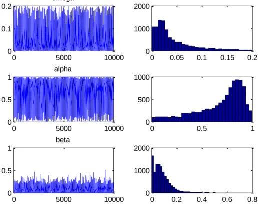
Figure 4: Histograms and draws of the posterior sample of the GARCH

parameters for XOM (M=10000)

Table 1: Parameters estimates for XOM (M=10000)

Parameters Estimates Quantiles ML estimates 0.05 0.5 0.95 Omega _(0.0421)0.0431 0.0025 0.0275 0.1398 0.0311 Alpha _(0.2387)0.8784 0.1611 0.7626 0.9418 0.8588 Beta _(0.0617)0.0766 0 0.0665 0.1937 0.0641

The table shows Bayesian estimates of the GARCH parameters of XOM obtained from M=10000 draws using Metropolis random-walk. The numbers in brackets are standard deviations.

The three following columns display the values of the quantiles of order 0.05, 0.5 and 0.95 obtain from the parameters distributions.

The last column shows the Maximum Likelihood estimators of the parameters.

0 5000 10000 0 0.1 0.2 omega 0 5000 10000 0 0.5 1 alpha 0 5000 10000 0 0.5 1 beta 0 0.05 0.1 0.15 0.2 0 1000 2000 0 0.5 1 0 500 1000 0 0.2 0.4 0.6 0.8 0 1000 2000

(17)

Posterior results obtained from the method for Exxon Mobil (XOM) are displayed in Table 1. They are fairly closed to the results obtained from the Maximum Likelihood estimation, but posterior means of , and seem a bit higher.

The history of sampled parameters shows that the values of the parameters are stationary around the zone of higher posterior probabilities.

Looking at the histograms of the distributions, we find that for the parameters and , the algorithm did not explore the tails of the distribution. Nevertheless, the peaks of all the distributions are located at the true values of parameters. This shows that the algorithm is converging.

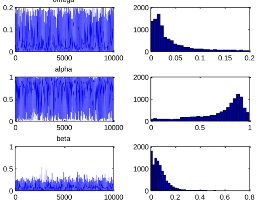
Figure 5: Histograms and draws of the posterior sample of the GARCH

parameters for TOT (M=10000)

0 5000 10000 0 0.1 0.2 omega 0 5000 10000 0 0.5 1 alpha 0 5000 10000 0 0.5 1 beta 0 0.05 0.1 0.15 0.2 0 2000 4000 0 0.5 1 0 1000 2000 0 0.2 0.4 0.6 0.8 0 1000 2000

(18)

Table 2: Parameters estimates for TOT (M=10000)

Table 2 shows posterior results for Total (TOT) as well as the Maximum likelihood estimates of its GARCH parameters. The table presents posterior means (the average of the sampled values) of the model parameters and the posterior standard deviations of the posterior means (the standard deviations of the sampled values).

The parameters estimates obtained by the method are fairly closed to the MLE’s. But unlike the parameters of Mobil (XOM) above, the posterior mean of in this case is smaller than its MLE counterpart. The quantile of order 0.5 is very closed to the estimators. This means that the median and the mean are fairly closed, a result that always characterize random variables with unimodal distributions.

The histograms illustrated in figure 5 display the same behavior as above with tin tails and peaks closed to the true values of the parameters.

Parameters Estimates Quantiles ML estimates 0.05 0.5 0.95 Omega 0.01053 _(0.0407) 0.0005 0.0142 0.1294 0.0089 Alpha _(0.2406)0.9044 0.1649 0.8496 0.9666 0.9239 Beta _(0.0539)0.0650 0 0.0558 0.1654 0.0541

The table shows Bayesian estimates of the GARCH parameters of XOM obtained from M=10000 draws using Metropolis random-walk. The numbers in bracket are standard deviations.

The three following columns display the values of the quantiles of order 0.05, 0.5 and 0.95 obtained from the parameters distributions.

(19)

Figure 6: Histograms and draws of the posterior sample of the GARCH parameters for CVX (M=10000)

Table 3: Parameters estimates for CVX (M=10000)

Parameters Estimates Quantiles ML estimates 0.05 0.5 0.95 Omega _(0.0417)0.0388 0.0017 0.0320 0.1377 0.0231 Alpha _(0.2373)0.8935 0.1840 0.8947 0.9577 0.8851 Beta _(0.0571)0.0699 0 0.0658 0.1654 0.0569

The table shows Bayesian estimates of the GARCH parameters of XOM obtained from M=10000 draws using Metropolis random-walk. The numbers in bracket are standard deviations.

The three following columns display the values of the quantiles of order 0.05, 0.5 and 0.95 obtain from the parameters distributions.

The last column shows the Maximum Likelihood estimators of the parameters.

0 5000 10000 0 0.1 0.2 omega 0 5000 10000 0 0.5 1 alpha 0 5000 10000 0 0.5 1 beta 0 0.05 0.1 0.15 0.2 0 1000 2000 0 0.5 1 0 1000 2000 0 0.2 0.4 0.6 0.8 0 1000 2000

(20)

Posterior results obtained by the sampling of the GARCH parameters of Chevron (CVX) are shown in Table 3.

In addition to the comments made in the preceding cases, the results show that the estimated values respect the positivity restrictions on the parameters while ensuring the positivity of the variance of the model variables. This result is also true for Mobil and Total.

The histograms of the posterior sample of the model parameters illustrated in figures 6 have the same behaviour as the previous ones described above.

For all those sampled parameters quantiles of order 0.05 appeared to be zero.

IV . 3 . Correlations estimates

We sampled data under Multivariate GARCH model with three elements subject at T=504 time points.

The empirical correlation matrix obtained from the data is:

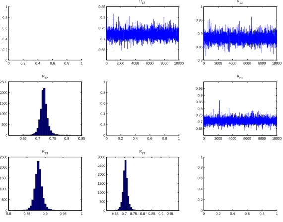
We launched the Metropolis chain of M=10000 accepted draws with the prior distribution on the unit vectors ’s forming the rows of the Cholesky matrices. The Metropolis-Hastings step was applied one by one to all the components of the correlation matrix.

Figures 7, which plot the posterior draws of the correlation elements of the correlation matrix, depict the behaviour of the parameters values during the sampling.

(21)

Figure 7: Plots of histograms and draws of the correlation matrix elements

Posterior results obtained by this sampling are shown in Table 5. The table presents posterior means (the average of the sampled values) of the correlation matrix elements and the posterior standard deviations of the posterior means (the standard deviations of the sampled values).

0 0.2 0.4 0.6 0.8 1 0 0.2 0.4 0.6 0.8 1 0 0.2 0.4 0.6 0.8 1 0 0.2 0.4 0.6 0.8 1 0 0.2 0.4 0.6 0.8 1 0 0.2 0.4 0.6 0.8 1 0 2000 4000 6000 8000 10000 0.65 0.7 0.75 0.8 0.85 R₁₂ 0 2000 4000 6000 8000 10000 0.8 0.85 0.9 0.95 1 R₁₃ 0 2000 4000 6000 8000 10000 0.65 0.7 0.75 0.8 0.85 0.9 0.95 R₂₃ 0.65 0.7 0.75 0.8 0.85 0 500 1000 1500 2000 2500 R₁₂ 0.8 0.85 0.9 0.95 1 0 500 1000 1500 2000 2500 R₁₃ 0.65 0.7 0.75 0.8 0.85 0.9 0.95 0 500 1000 1500 2000 2500 3000 R₂₃

(22)

Table 4: Posterior Correlation Matrix (means and standard deviations) of the M-GARCH model obtained with M=10000 accepted draws

XOM TOT CVX

XOM 1 _(0.0128)0.7224 _(0.0107)0.8829

TOT 0.7204** 1 _(0.0137)0.7167

CVX 0.8820** 0.7066** 1

The table shows Bayesian estimates of the GARCH Correlation coefficients obtained from 10000 draws using Metropolis random-walk. The numbers in bracket are standard deviations.

**The lower triangular matrix shows the Empirical correlation coefficients.

The posterior means of the elements of the correlation matrix respect the classical restrictions and ensure the positive definiteness of the correlation matrix. Furthermore, the coefficients of this matrix have values closed from their empirical correlation matrix counterpart, and this can be explained by looking at the histograms of the posterior sample of correlation elements (see Figures 7 above). because the posterior distributions for all the coefficients are closed to normality, the estimates of the parameters and the corresponding standard deviations have a straightforward interpretation.

In summary, the results of our algorithm have the following features:

- the estimated parameters of interest converge to a flat region of higher posterior probability and then fluctuate around that region.

- Histograms tends to have a normal shape with peaks closed to the value of the estimates

(23)

- The estimated parameters are closed to their MLE counterparts

- All the constraints on parameters and correlation coefficients and matrix are respected a posteriori

V. CONCLUSION

In this study, we provide an empirical analysis of the Multivariate GARCH model with constant conditional correlation. We use financial data from three daily stock returns from the energy sector of the New York stock market to apply the method. The estimation of the parameters of the models together with the correlation matrix under consideration is obtained by using the Random Walk chain Metropolis-Hastings algorithm together with a geometrical approach of computing the linear correlations. We provide detailed guidelines on how to construct the required Markov chains using Metropolis–Hastings steps.

Under a Bayesian framework, we then construct samples of the GARCH parameters and the Correlation Matrix elements which have as stationary distributions the posterior distributions of the model. Finally, we find that this algorithm is computationally efficient and provide good posterior samples as the estimated parameters converge to a flat region near the true parameters, respect the required constraints of positivity, positive definiteness and boundedness, and yield posterior probability distributions that are easy to interpret.

(24)

References

[ 1 ] Barnard, J., McCulloch, R. and Meng, X.L. (2000). Modeling covariance

matrices in terms of standard deviations and correlations with application to shrinkage. Statistica Sinica 10, 1281-1311

[ 2 ] Bollerslev T, Chou RY, Kroner KF. 1992. ARCH modeling in finance—A

review of the theory and empirical evidence. Journal of Econometrics 52: 5–59.

[ 3 ] Bowen, L. and Lombrano, M. (1998). Bayesian inference on GARCH

models using the Gibbs sampler. Econometrics Journal Vol 1, c23-c46

[ 4 ] Chib, S. and Greenberg, E. (1995). Understanding the Metropolis-Hastings

Algorithm. The American Statistician, Vol. 49, No. 4. pp. 327-335.

[ 5 ] Chib, S. and Greenberg, E. (1998). Bayesian analysis of multivariate probit

models. Biometrika 85, 347-361.

[ 6 ] Daniels, M.J. and Kass, R.E. (1999). Nonconjugate Bayesian estimation of

covariance matrices and its use in hierarchical models. Journal of the American Statistical Association 94, 1254-1263.

[ 7 ] Gourieroux, C. (1997). ARCH Models and Financial Applications. New

York, Springer Verlag

[ 8 ] Koop, G. Bayesian Ecoometrics; Wiley

[ 9 ] Liechty, J., Liechty, M., and Muller, P. (2004). Bayesian

Correlation Estimation. Biometrika 91,1-14

[ 10 ] Liu, X. & Daniels, M. (2007). A new algorithm for simulating a

correlation matrix based on Parameter Expansion and Re-parametrization. Department of Statistics, University of Florida

[ 11 ] Nzabandora, W. (2007). Estimation bayesienne des matrices de correlations:

strategies de formulation de lois a priori. Department de Sciences Economiques, Universite de Montreal

[ 12 ] Tim Bollerslev (1990). Modelling the Coherence in Short-Run Nominal

Exchange Rates: A Multivariate Generalized Arch Model. The Review of Economics and Statistics, Vol. 72, No. 3. pp. 498-505.

[ 13 ] Tse, Y. and Tsui, K. (2000). A Multivariate GARCH Model with

(25)

Singapoore

[ 14 ] Vrontos, I., Dellaportas, P. and Politis, D. (2003).Inference for some

(26)

Bayesian estimation of correlation matrices: Application to the Multivariate GARCH model