This is an author-deposited version published in: https://sam.ensam.eu Handle ID: .http://hdl.handle.net/10985/7617
To cite this version :
Koji HIRANO, Rémy FABBRO - Experimental investigation of hydrodynamics of melt layer during laser cutting of steel - Journal of Physics D : Applied Physics - Vol. 44, p.105502 - 2011
Experimental investigation of hydrodynamics of melt
layer during laser cutting of steel
Koji Hirano 1,2, Remy Fabbro 1
1 PIMM Laboratory (Arts et Métiers ParisTech-CNRS), 151 Boulevard de l’Hôpital 75013 Paris, France.
2 Nippon Steel Corporation, Marunouchi Park Building, 2-6-1 Marunouchi, Chiyoda Ward, Tokyo 100-8071, Japan.
Email: hirano.koji@nsc.co.jp
Abstract. In laser cutting process, understanding of hydrodynamics of melt
layer is significant, because it is an important factor which controls the final quality. In this work, we observed hydrodynamics of melt layer on kerf front in the case of laser cutting of steel with inert gas. The observation shows that the melt flow on the kerf front exhibits strong instability, depending on cutting velocity. In intermediate range of velocity, the flow on the central part of the kerf front is continuous, whereas the flow along the sides is discontinuous. It is firstly confirmed that the instability in the side flow is the cause of the striation initiation from the top part of the kerf. The origin of the instability is discussed in terms of instabilities in thermal dynamics and hydrodynamics. The proposed model shows reasonable agreement with experimental results.
Keywords: Laser cutting, Hydrodynamic instability, Surface tension, Striations. PACS: 42.62.-b, 81.20.Wk
1. Introduction
Since its invention in the 1960’s, laser cutting of steel has widely been used in industries owing to its advantage of processing speed or capability of automation. Along with the applications, a number of researches have been conducted to understand fundamental mechanism of the process. Now there exist global process models, which can predict achievable thickness or velocity depending on operational parameters [1-3].
However, our understanding of the time-dependent fluctuation (instability) is not sufficient. For example, we have not reached a conclusion on mechanism of striation generation, which is a major quality problem in laser cutting of steel. Recently the subject has become more important, because it has been revealed that new promising fibre or disk lasers cannot offer the same quality as conventional CO2 lasers in case of thick steel cutting [4, 5]. The above-mentioned models deal with stationary condition based on several equilibrium balances, so that they cannot predict instability. Fundamental investigations on instability from both experimental and theoretical sides are being required.
Concerning the striation generation, we understand the mechanism well in the special case of using oxygen, which provides the exothermic energy. The model of cyclic activation and extinction of oxygen combustion, which was proposed by Arata et al [6], was raised up to the level of numerical modelling [7, 8] and they can explain striations created on kerf sides.
It has been well acknowledged that the striations do not vanish even when we reduce the content of oxygen in assist gas [9]. Although the mechanism of striation generation for the case with inert gas might be simpler, in that it involves only heat input by laser beam, the mechanism has remained unknown for several decades.
In spite of the lack of consensus, several types of mechanisms have been suggested theoretically to explain the striation generation in the case of steel cutting with inert gas. One idea is to attribute the striations to external fluctuation of operating parameters such as laser power and gas flow rate, which can change the energy and momentum balances [10, 11]. But this does not seem to be a primary mechanism, considering the fact that the striations have excellent regularity in most cases and that typical pitch (wavelength) of striations is in the range of 100 m regardless of laser and gas systems. Another mechanism is hydrodynamical instability induced in the melt layer during its interaction with gas jet [12, 13]. This can be a mechanism which causes the creation of striations in lower part of kerf, where the melt layer becomes thicker and the gas flow less stable. However, it seems that the initiation of the striations at the top part of the kerf should be driven by another physical process. More promising candidate is the instability of thermal dynamics, which generates bunches of molten material (humps) sliding down the kerf front [14-18]. This seems to be promising to explain the initiation of striations, because it is related to the peculiarity of temperature field around the top part of the kerf. There are still two points that are not clear, however; one is the fact that the theory predicts that the instability occurs only in low speed range, and the other is that it is not so trivial whether the instability on the front perturbs the dynamics on the kerf side.
Although experimental observation is essential to reach correct description of the mechanism, there have been few such investigations. Meanwhile, a recent study by Yudin et al [19] showed an interesting result. CO2 laser cutting was conducted with Rose’s alloy, which has low melting temperature. They observed the kerf side through a glass plate, which was attached onto the sample. They observed melt structure, which they call stalactites, sliding down perpendicularly along the kerf side. The striations were generated during resolidification of the stalactites. In low gas pressure and high cutting velocity conditions, they observed ripple formation near the bottom part of the kerf, which is another mechanism of striation generation. However, precise observation of the top part of the kerf was not realised, so that it could not be revealed why the striations are generated from the top surface, in other words, why stalactites emerge periodically.
A primary object of this work is to clarify the mechanism of striation initiation from the top part of the kerf by experimental observation of the kerf front. Using high-speed video technique, we observe both the kerf front and kerf side simultaneously from the above of the sample. In the next section 2, the experimental setup is explained. In the section 3, the obtained films are presented with some analysis of characteristic parameters. The section 4 is devoted to discussion on the origin of observed instability.
2. Experimental setup
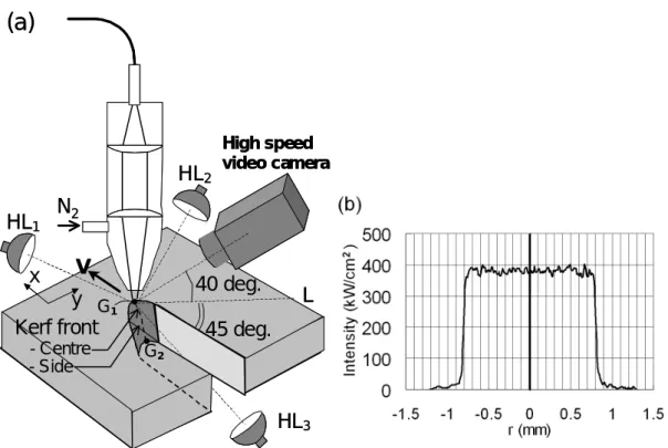
Schematic of experimental apparatus is shown in figure 1(a). A 10 kW disk laser (Trumpf, TruDisk10002) was used as laser beam source. The laser power was fixed at 8 kW throughout this work. After passing through a multimode-fibre with the diameter of 0.6 mm, the laser beam was collimated and focused onto a sample. The focal distances of the collimation lens and focusing lens were 200 mm and 560 mm, respectively. Thus the focus diameter df at the sample was 1.7 mm. The beam profile at the focus position was measured with a commercial CMOS camera. The result is shown in figure 1 (b), where the top-hat distribution of the intensity is confirmed.
We chose the focal spot diameter, which is larger than diameter typically used (~0.1 mm). It could have been possible to utilise such small focus diameter, but it is a very difficult task to observe the dynamics of phenomenon with sufficient spatial resolution. Instead of increasing the magnification factor of the optical system of the camera, we adopted a much easier way to enlarge the spatial scale of the kerf, in order to have a better visualization and to deduce the mechanism of the striation generation. Despite the increase of diameter, relevant physical processes or mechanisms are not expected to change so much, since most of the physical processes of heat transfer in solid and liquid layer and of hydrodynamics in liquid are scalable in terms of governing mathematical equations.
Low carbon mild steel was used as samples. The thickness was 3 mm, and the very surface layer of steel oxide had been removed by mechanical polishing to avoid unfavourable perturbations. Nitrogen was used as assist gas, which was ejected from an ordinary circular nozzle with the exit diameter of 3.5 mm. The stand-off distance of the nozzle was set at a rather large value of 3.5 mm, to assure the vision around the kerf. The pressure of gas in the nozzle was 2.5 bar, so that the gas flow from the nozzle was free from shock waves, which would have introduced disturbances in the flow. The flow rate was measured to be Q = 115 L/min. with a standard gas flow meter, taking into account density correction due to the gas pressure. The pressure distribution at the sample position (3.5 mm below the exit surface of the nozzle) was measured with a Pitot tube. The total pressure Ptot showed 2.4 bar on the nozzle axis. The pressure distribution was homogeneous within df (1.7 mm) and the distribution had diameter dg of 4.8 mm measured at FWHM. Assuming that the size of pressure distribution corresponds to that of velocity field, the gas velocity at the top surface of the kerf can be estimated from the following formula: High speed video camera
N
2V
45 deg.
Kerf front
- Centre - Side40 deg.
L
x
y
(a)
G1 G2HL
1HL
2HL
3 High speed video cameraN
2V
45 deg.
Kerf front
- Centre - Side40 deg.
L
x
y
(a)
G1 G2HL
1HL
2HL
3Figure 1. (a) Scheme of the experimental setupand (b) intensity distribution of focused beam on sample surface. In (a), HL1~3 represent halogen lamps used for illumination.
4
2 g gd
Q
v
(1) which gives vg = 1.1 x 10 2m/s. The static pressure Pin at the entrance of the kerf is estimated from the Bernoulli’s equation for compressible gas flow [20]:
1 0 0 1 2 1 0 0 11
2
1
1
P
P
v
P
P
tot g in (2) Here γ is the adiabatic exponent (=1.4 for N2) and 0 is the density of N2 at ambient pressure P0 = 1 x 10⁵ Pa (0 = 1.3 kg/m3
). Inserting these values to (2) one obtains Pin = 2.1 bar.
As mentioned above, in order to have intact vision and stable gas flow, we used the large stand-off distance and the low pressure as compared to the standard practice of inert gas laser cutting. This means that gas force exerted on melt layer was lower. Nevertheless, striations observed in this study are essentially the same as in practical conditions, as will be shown. Moreover, the influence of gas parameters on the striation generation process will be discussed in the section 4.3.
The kerf front was observed by a high speed video camera (Photron, FASTCAM/APX-RS) with the acquisition rate of 20 kHz. In order to clarify the initiation process of striations, the top part of the front was observed from the above, with the angle of 40 degree with respect to horizontal surface. To visualise the central and side parts of the kerf front at the same time, the angle of the observation was deviated by 45 degree from the cutting direction (Please note also our notations concerning parts of the kerf, which are presented in figure 1 (a)). The spatial resolution of the video images was approximately 10 m/pixel. As shown in figure 1(a), three halogen lamps (HL1~3) were used for illumination; the two HL1 and HL2 from the above of the sample to illuminate the sample surface and the side part of the kerf front, respectively, and the other HL3 from the below through the kerf to illuminate the central part of the front. No wavelength filter was used. The exposure time was set at 0.05 ms, the inverse of the acquisition rate.
The cutting speed V was varied from 1 m/min to 6 m/min to investigate the evolution of hydrodynamics. The roughness Rz and the wavelength of striations were measured along lines located at 0.5 mm below the top surface. We measured also tilting angle of kerf front with samples obtained after switching-off of the laser beam. The angle was evaluated as the value averaged over the sample thickness, using a straight line which links the two points G1G2 on the top and back surfaces (see figure 1(a)). In the case where the sample could not be cut through, the lower point G2 is substituted by the end point of the tilted kerf front. The technique gives rather accurate estimation of , since melt layer is so thin that it is frozen very rapidly when the laser is turned off. (The thickness sm of the melt layer can be estimated in the order of 100 m from the mass balance equation smVm = DV [21], where D is the workpiece thickness (3 mm) and Vm is the velocity of continuous melt flow, which will be shown later in figure 4.) The freezing time of the melt layer was confirmed experimentally to be roughly 0.2 ms by the high speed video observation. The melt layer moves only several hundred microns after the turn-off of the laser if we multiply the freezing time by measured velocity of melt layer (1~3 m/sec).
3. Results
Typical examples of images acquired for different cutting velocities V from 1 m/min to 6 m/min are shown in figure 2. As can be seen, liquid flow on the kerf front exhibits strong dependence on V. In the following, we describe observed phenomena for several different velocity ranges. For the present operating conditions, the maximum speed to cut through the 3 mm thick was V
= 3 m/min. Even in the range of V > 3 m/min, however, the flow feature observed in this top part of the kerf is considered to be essentially the same as that would be obtained when the thinner samples are to be cut properly.
3.1. Velocity dependence of hydrodynamics (i) V = 3 m/min
Let us start from the intermediate case of V = 3 m/min (figure 2(c)). Two different flows can be recognized: the flow in the central region of the kerf front and the flow on the side of the kerf. In the following, we call the former the central flow, and the latter the side flow. We define W,
(d)
(b)
(a)
B
1B
2S
(e)
C
(c)
P
L
F
W
α
R
E
(d)
(d)
(b)
(b)
(a)
B
1B
2S
(a)
B
1B
2S
(e)
C
(e)
C
(c)
P
L
F
W
α
R
E
(c)
P
L
F
W
α
R
E
Figure 2. Observation result for different velocities V. (a) V = 1 m/min, (b) V = 2 m/min, (c) V
= 3 m/min, (d) V = 4 m/min and (e) V = 6 m/min. For the scale of the images, refer to the kerf width dk in figure 3 (dk ~ 1.7 mm for all the V).
0 10 20 30 40 50 60 70 0 2 4 6
Cutting Velocity V (m/min.)
α
( de gr ee ) 0 0.04 0.08 0.12 0.16 0.2 0.24 0.28 W idt h sd
k , W ( m m ) 1.6 1.7 1.8d
k Wα
expα
th 0 10 20 30 40 50 60 70 0 2 4 6Cutting Velocity V (m/min.)
α
( de gr ee ) 0 0.04 0.08 0.12 0.16 0.2 0.24 0.28 W idt h sd
k , W ( m m ) 1.6 1.7 1.8d
k Wα
expα
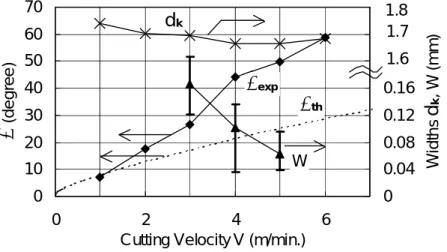
thFigure 3. Velocity dependence of tilting angle of kerf front; experimental measurement (exp) and theoretical prediction from the equation (9) (th). Also shown are measured values of kerf width (dk) and the width of unstable side region (W).
the thickness of the side flow region, as the distance from the kerf side line to the point R on the kerf, which separates the continuous central region and discontinuous side region. In the present case of V = 3 m/min, W = 160 m.
The central flow runs continuously and smoothly downwards along the central part of the kerf. The central symmetrical line on the kerf is tilted by an angle of 26 degree with respect to the beam incident axis (see also figure 3). The velocity of the continuous flow is determined as 3.2 m/s using moving particles like P in figure 2(c), which appear occasionally (see also figure 4). We think that they are some very small inclusions inside the material, but the characteristics such as chemical composition and size are not clear at the present stage.
On the other hand, the flow in the side region between the points L and R in figure 2(c) exhibits striking discontinuity and periodicity. The termination point L on the left corresponds to the edge of overlapped region with laser beam, whose position at the surface is shown on figure 2(c) by the ellipse (df = 1.7 mm). The point R is located at the separation point of the central and side flows. The very top part of the region is very bright because of specular reflection from the halogen lamp HL2 (see figure 1(a)). Liquid accumulations are generated one by one from the top part and displaced towards the direction shown with F in the figure; they slide down on the sidewall of the kerf until they are absorbed by the central flow. After displacement of each accumulation, one single vertical stripe of striations is created on the sidewall. The depth of region where we observe such vertical striations (distance E in figure 2(c)) is determined by the travelling distance of accumulations before joining to the central flow. The average time interval ta of two accumulation generations was measured to be 4 ms. The wavelength of striations measured after cutting was 199 m, which corresponds to the value of V·ta = 200 m. It is clear that the periodical generation and displacement of accumulations is the origin of the striations. Whereas Yudin et al [19] already observed the downward displacement of the accumulations by lateral visualisation of the kerf side through a transparent glass, our observation has revealed for the first time the processes of the accumulation generation and the striation initiation at the top part of the kerf. More detailed description of the striation generation process is given in the next section 3.2.
(ii) 3 m/min < V < 6 m/min 0 0.5 1 1.5 2 2.5 3 3.5 4 4.5 5 0 2 4 6
Cutting Velocity V (m/min.)
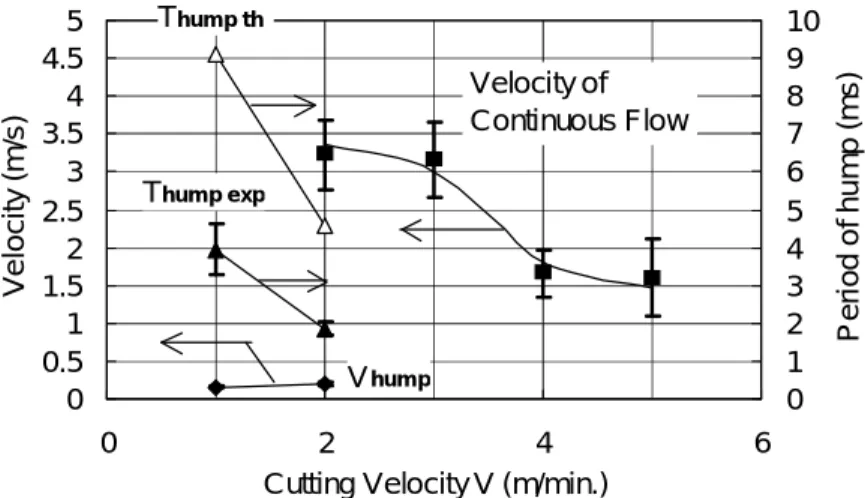
V e lo c it y ( m /s ) 0 1 2 3 4 5 6 7 8 9 10 P e ri o d o f h u m p ( m s ) Velocity of Continuous Flow Vhum p Thum p th Thum p exp
Figure 4. Measured velocities of continuous flow and humps in the central region of the kerf
front. Measured values of periods of humps (Thump exp) are also shown with theoretical prediction from the equation (14) (Thump th).
When the velocity is increased from 3 m/min to 5 m/min (figure 2(d)), general feature of the flow does not change. The stable central flow and the non-stationary side flow exist and the periodic behaviour of the latter generates regular striations on the side. Meanwhile, characteristic parameters of the flow depend on the cutting velocity V. As shown in figure 3, the tilting angle of the front at the centre line increases with V and at the same time, the thickness W of unstable side region decreases. Because of this increase of , the travelling distance of accumulations before meeting the central flow becomes shorter. The depth of region where we observe regular vertical striations is thus reduced. The wavelength of striations slightly decreases with this increase in V (see figure 5).
(iii) V = 6 m/min
If we further increase V to 6 m/min (figure 2(e)), the stable central flow covers the entire kerf front, and the periodic generation of accumulations and their downward displacement along the kerf side cannot be observed any more. Correspondingly, no striation appears on the side, although we observe random oscillation of the liquid surface level of the central flow, which creates very thin relief.
Let us mention here some fundamental remarks about the velocity of the continuous central flow. As shown in figure 4, the velocity decreases with increasing V. At V = 6 m/min, we could not determine the velocity because we found no particles moving downwards. Instead, we found particles moving laterally along the semi-circular kerf shape as designated with C in figure 2(e). It is likely that this change of flow is caused by combination of the following two factors. First, as the tilting angle of the front increases with V (figure 3), the laser beam intensity absorbed on the central part increases, so that the azimuthal flow to the side by the piston mechanism [22] becomes relatively important compared with the downward flow. Second, as increases, the deflection of gas flow near the front surface becomes more pronounced. As a result, the tangential force which is applied on the melt surface is considered to be decreased.
(iv) V = 2 m/min
On the other hand, when V is decreased from 3 m/min, the central part also begins to show discrete behaviour, as is clear in the case of V = 1 m/min (figure 2(a)). The melt flows down intermittently; parts of surface between the two successive bunches of melt are not even covered with liquid metal. We will define these liquid bunches as humps in this paper. The threshold
0 50 100 150 200 250 300 350 400 450 500 0 2 4 6
Cutting velocity (m/min.)
0 20 40 60 80 100 120 140 160 180 200 R o u g h n e s s R z ( μ m ) λexp Rz th Rz exp S tr ia ti o n W a v e le n g th ( m ) 0 50 100 150 200 250 300 350 400 450 500 0 2 4 6
Cutting velocity (m/min.)
0 20 40 60 80 100 120 140 160 180 200 R o u g h n e s s R z ( μ m ) λexp Rz th Rz exp S tr ia ti o n W a v e le n g th ( m )
Figure 5. Measured striation wavelength exp and surface roughness Rz exp. For Rz, theoretical prediction Rz th from eq. (27) is also presented.
velocity of the appearance of this discontinuity is V = 2 m/min, where the flow in the central region fluctuates between the two regimes of continuous and discontinuous flows. An interesting point is that, at V = 2 m/min, the velocity of continuous flow was observed to be 3.2 m/s, whereas the velocity of humps was 0.2 m/s. It is not surprising to observe this difference, because the evolution of hump is not a mass flow but an evolution of phase as already pointed out [15, 16, 18].
The image at V = 2 m/min shown in figure 2(b) is the one typically observed when the central flow is in the continuous regime. Compared with V = 3 m/min, the angle is decreased (see also figure 3). This leads to the extension of perpendicular striations which are left on the kerf side. At the same time, the width W of unstable side flow as well as the accumulation size becomes larger. Travelling paths of the accumulations are more irregular and complex. The accumulation surrounded with a white dotted line in figure 2(b) shows such an example: several branches originate from the single accumulation, one of which goes away to the left without being absorbed to the central flow. As a consequence of this kind of irregularity, striation relief which is left on the kerf side is not as regular as in the case of V > 2 m/min.
(v) V = 1 m/min
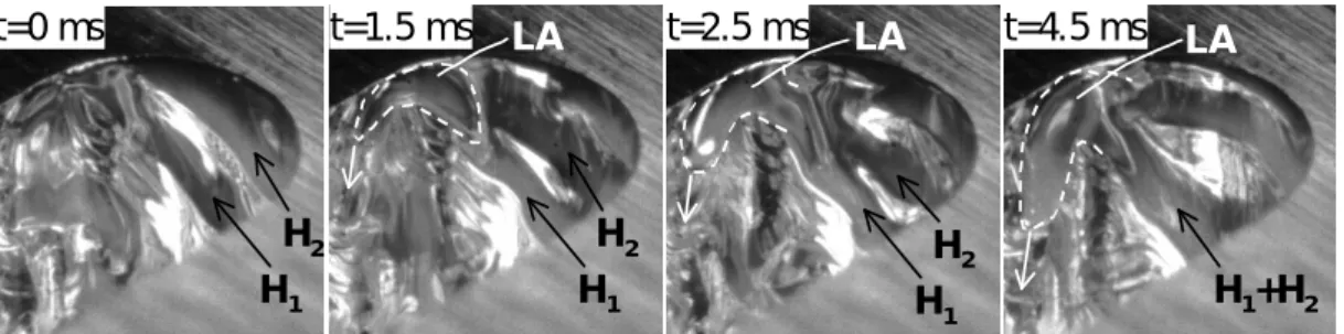
When we further decrease V to 1 m/min, the central flow completely becomes the regime of humps. Now the melt flow is discontinuous on the entire kerf front. The dynamics of the humps and accumulations becomes more and more irregular, and they show stronger interactions to each other. In the central region, humps, which are generated from the top part at every 4 ms, slides down with velocity of 0.15 m/s. Compared with V = 2 m/min, the generation time period is doubled, so that the pitch measured along the cutting direction (x-axis) stays at the same value of 70 m. It is frequently observed that two successive humps starting from the surface merge in the middle of the front and go down together after that. Such an example can be found in a sequence of images shown in figure 6. The two humps H1 and H2 are separated at t = 0 ms. At t = 1.5 ms, however, they begin to interact via the liquid accumulation LA on the side. The merger is initiated and they are completely unified at t = 4.5 ms. In figure 6 one can observe also a branch of the liquid accumulation (LA) escaping to the left.
Another interesting feature is found in bright regions such as those marked with B1 and B2 in figure 2(a). These regions are not covered with liquid but are very bright because the light emitted from the halogen lamp HL3 is specularly reflected in these regions toward the video camera. The centre lines B1 and B2 of the two bands have a lag, which indicates that the hump is situated on a small plateau S, whose tilting angle is different from the two parts above (B1) and below (B2). This difference of the tilting angle is also suggested from the difference in the brightness. The solid regions are bright since the angle matches that of the specular reflection from HL3, while the liquid on S is less bright due to the mismatch of the angle. It has been
t=0 ms t=1.5 ms t=2.5 ms t=4.5 ms H1 H2 H1 H2 H1 H2 H1+H2 LA LA LA t=0 ms t=1.5 ms t=2.5 ms t=4.5 ms H1 H2 H1 H2 H1 H2 H1+H2 LA LA LA
Figure 6. Example of melt accumulation dynamics observed for V = 1 m/min. A merger of
two successive humps H1 and H2 is shown. The white dotted lines indicate approximate border of the liquid accumulation LA. As for the scale of the images, note that dk = 1.74 mm.
already discussed that the regime of humps involves such plateaus around the humps [14-18]. (vi) Summary of velocity dependence
Table 1 summarises the observed different regimes, which are classified from the viewpoint of instability. When V is increased from 1 m/min, the whole region on the kerf front exhibits discontinuity until V = 2 m/min. In the following intermediate velocity range from 2 m/min to 6 m/min, the central flow becomes continuous, but the side flow is still discontinuous. As V increases, the width W of the unstable side region diminishes with the expansion of the stable central region. The side flow in this regime is characterised by periodic generation of accumulations at the top part and their displacement downwards, which is the origin of regular vertical striations created on the kerf sides. And finally, the unstable side region disappears at V = 6 m/min.
The existence of instability in the central region has been predicted theoretically for low velocity condition [14, 17]. Meanwhile, an important point firstly shown by the present observation is that there is a regime where we observe simultaneously both the stable and unstable flows, in the central and side regions, respectively. In most of the theoretical works in the past, it has been assumed that the instability in the central part naturally perturbs the flow in the side region [14-17]. This kind of assumptions should be rejected for the intermediate regime.
Table1. Velocity dependence of the flows.
Cutting Velocity V (m/min) V <2 2<V <6 V =6 Central flow Unstable Stable Stable Side flow Unstable Unstable Stable
3.2. Process of striation generation
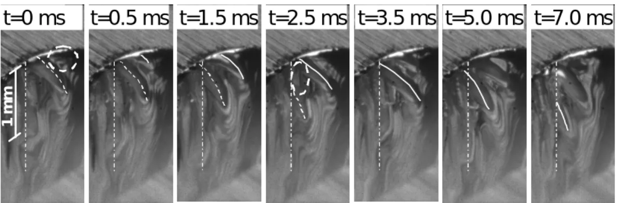
Let us see more precisely the striation generation process. An example of the generation, development and displacement of an accumulation for V = 3 m/min is shown in figure 7. The solid lines indicate the position of the accumulation under consideration at each time. The dotted lines show the position of the precedent accumulation. The dot-dash lines show the border of laser beam overlap region. In the first image at t = 0 ms, no accumulation is
t=0.5
t=1.5
t=0 ms
t=0.5 ms
t=1.5 ms t=2.5 ms t=3.5 ms t=5.0 ms t=7.0 ms
1 m mt=0 ms
t=0.5
t=1.5
t=0 ms
t=0.5 ms
t=1.5 ms t=2.5 ms t=3.5 ms t=5.0 ms t=7.0 ms
1 m mt=0 ms
Figure 7. Dynamics of an accumulation observed at V = 3 m/min. The solid and dotted lines
show the position of the accumulation under consideration and the precedent accumulation, respectively. The dotted circle at t = 0 ms indicates the position of the creation of the accumulations. The dotted ellipse at t = 2.5 ms shows a ridge left after the displacement of the precedent accumulation.
recognized inside of the white dotted circle, from which the precedent accumulation has just gone out. At t = 0.5 ms, the new accumulation is confirmed in this region and it continues to grow up. At t = 1.5 ms, one can see that the bottom of the accumulation now touches the central flow. The displacement of this accumulation seems to be dragged by the central flow after this time. The accumulation continues to descend and finally it is sucked into the central flow at t = 7.0 ms. After the displacement of such accumulation, one single stripe of the striation structure is left on the kerf side.
Why do the accumulations go down quite vertically? The observation suggests the following two guiding mechanisms on the displacement of accumulations by downward gas force. Firstly the accumulations cannot go beyond the border of the beam (dot-dash lines), because they cannot exist as liquid any more once they do so. The cooling rate of the liquid is very rapid, as will be shown in the section 4.3.3. In addition, there is a geometrical effect. The white dotted ellipse in the image at t = 2.5 ms surrounds a vertical line, which corresponds to a ridge of the striations. The height of such ridge can be estimated from the surface roughness. The measured value of Rz is 40 m in this case of V = 3 m/min (see also figure 5). From the images which follow after t = 2.5 ms, it appears that the ridge works as a guide, preventing the accumulation from passing over the ridge. Thus the displacement of the present accumulation is again perpendicular to the top surface of the sample, reproducing a new ridge on the other side. In summary, the observation has clarified for the first time the generation process of vertical striations. This regular process applies to the velocity range of 2 m/min < V < 6 m/min. For the lowest velocity range (V < 2 m/min), the accumulation is also generated rather periodically at the top part of the kerf, but the irregularity of accumulation trajectory perturbs final relief left on the kerf side.
4. Discussion
4.1. Tilting angle of central part
It is considered that the tilting angle of central part of the kerf front, which increases with cutting velocity V, plays an important role in determining the stability of the flow, as discussed in the following.
Let us consider first the dependence of the angle on V. This can be considered from the equation of power balance per unit length along kerf depth, which is written as
l m s
a p p p
p (3) All the terms have the dimension of W/m. The term pa in the left side is the energy input to the system per unit depth. It can be approximated using the incident laser intensity IL, the absorptivity A, the radius rk of the kerf front (rk ≈ df /2) and the mean tilting angle :
)
2
tan
(
L ka
A
I
r
p
(4) We have taken (2rk) as the characteristic length of the part along the kerf front which receives laser beam, neglecting its dependence on depth from the surface. The first and second terms on the right hand side of (3) represent the powers necessary to heat the solid material of the kerf part up to the melting temperature Tm and to heat it further to Tl, which is the mean temperature of liquid:
k
ps
m
m
s s V r C T T L p
2 0 (5)
k
pl
l m
l m V r C T T p
2 (6) Here T0 is the initial temperature, and Lm is the latent heat, and s (l), and Cps (C pl) are the density and heat capacity of solid (liquid), respectively. The third term in the right hand side of the equation (3) is the power lost by heat conduction into the solid part, which can be expressedas [23]
3 . 0 0 2 4 K T T Pe pl m (7) Here K is heat conductivity of the material. And
V r
Pe k
(8) is the non-dimensional Peclet number. From the equations (3)-(8), one obtains
3 . 0 0 0 2 4 2 tan 2 ) ( C T T L C T T Pe K T T Pe r I A
L k
s ps m
s m
l pl l m m (9)The right hand side is increasing function of Pe. Noting that Pe is proportional to V, the expression shows that for a given conditions of IL and rk, the angle increases monotonously with the increase of V. Although we have unknown parameters A() and Tl, we dare estimate the angle with assumption that A is constant at 0.5 regardless of and also that Tl = Tm. The result is shown in figure 3 as the dotted line. The model predicts well the increase of with V. The discrepancy between this tentative plot and the experiment increases as V increases and this must be attributed to the assumption of Tl = Tm. Thus it is implied that the temperature Tl of melt layer increases monotonously with V, as is usually observed in experimental temperature measurements [6, 24].
4.2. Instability in the central part (hump generation)
Let us consider first the origin of the humps, which were observed in the central part for low cutting speed V < 2 m/min. As shown in the following, the instability can be explained from combination of two phenomena: instability in thermal dynamics related to melting process and instability in hydrodynamics of the produced molten material. This idea of the combination of the two physical processes was already proposed by Golubev [17].
4.2.1. Instability in thermal dynamics
It is predicted that for low velocity condition, melting and ejection cannot occur homogeneously on the kerf front, but occurs locally, due to inherent instability in thermal dynamics [14, 17]. This situation is schematically explained in figure 8(a), which shows the solid-liquid interface at the centre line of kerf front at some instance. Please note that the molten metal is not taken into account yet and not depicted in the figure.
Time evolution of the profile is explained as follows. First, local melting at the top part creates a small plateau so-called “shelf” [17]. This shelf structure slides down along the kerf front, because the absorbed intensity is higher on the shelf than other part and local drilling occurs there. Periodical generation of such shelves from the top part generates wavy structure in the solid-liquid interface, which propagates downwards.
As is observed for V = 1 m/min (figure 2(a)), melting tends to occur only in the vicinity of the shelves. The reason can be explained as follows. First let us pay attention to the time-averaged value ave, which is shown by the dotted line in figure 8(a). This mean angle corresponds to the equilibrium tilting angle, which satisfies the power balance (eq. (9)). Due to the existence of shelves, regions between any two shelves must have local tilting angle that is lower than the time-averaged value ave, so that the regions between the shelves must be cooled and cannot be melted. Consequently, the melt accumulations (humps) exist only on the shelves and they are transported downwards with the displacement of the shelves. If we take a look at the evolution of the solid-liquid interface at certain depth, the advance of the interface along the cutting
direction occurs only when the shelves pass the point. The downward velocity of the shelves (humps) can be roughly estimated as [17]
ps m m
s L humpL
T
T
C
AI
V
0
(10)The equation assumes horizontal shelves (~ 90 degrees) and neglects preheating in solid and temperature increase over Tm in the melt layer. It predicts Vhump = 0.25 m/s, for the absorptivity A = 0.5. The value is in the same order as the velocity observed experimentally (0.15 ~ 0.2 m/s). 4.2.2. Instability in hydrodynamics
The important outcome of the localised melting is that molten metal cannot exist as continuous layer but as humps. Supposing that we have such instability, then what determines the typical size or period of the humps generated at the top part of the central region? To consider this problem, we now take into account the hydrodynamics of molten material. We will discuss about the force balance between surface tension and dynamic force exerted by gas, in a similar way as in the work by Makashev et al [15, 16].
Let us consider the condition which is necessary to trigger the displacement of a hump from the top surface, using a simple model described in figure 8(b). At time t = t0, the precedent ejection cycle is over and there rests no melt inside the area of laser beam. As the laser beam proceeds after this time, solid part comes into the beam area and is melted rapidly. When the size of melt accumulation is too small, surface tension force remains larger than the gas force, which is applied from the above, so that the accumulation continues to stay attached at the top. As laser beam proceed, more melt is generated and its size grows up. The gas force increases due to the increase of its surface area ·l, where and l are the dimensions of the accumulation (figure 8(b)). The accumulation is considered to start to move when the gas force exceeds the surface tension force ·l that retains the accumulation along the distance l. This balance can be
(b)
l
Gas
Laser beam position at t=t0V
x
V
(a)
α
ave Intensity distribution of laser beamJ
(b)
l
Gas
Laser beam position at t=t0V
x
V
(a)
α
ave Intensity distribution of laser beamJ
Figure 8. Schematics of profiles of solid-liquid interface on the cross section of the central
plane of the kerf (a) and of melt accumulation at the top part of the central region of the kerf (b), viewed on the cross section of the central plane (upper) and from the above (lower).
expressed as
l
l
F
s
(11) where Fs is the force per unit area applied on the surface of the accumulation. The applied surface area is measured by the projection to the sample surface (·l). The Fs per unit area is generally composed of viscous friction and static pressure. Makashev et al [15, 16] considered that Fs is expressed by pressure drop across the vertical length of the accumulation (~), which is caused by the reduction of gas flow cross section S due to the existence of the accumulation. However, it is not so evident how to estimate the change S, because the gas flow can expand freely inside the kerf along the cutting direction. Moreover, in the present study, relative variation (S/S) of the cross section, which might be expressed as (rk), is so small that the estimation of (S/S) is very delicate. The relation (rk) << 1 suggests that, instead of considering (S/S) for the entire gas flow, it should be more appropriate to look at the problem locally; in such a way that force is exerted on an obstacle placed within a homogeneous one-directional flow. According to a classical theory explaining drag force, Fs can be written as [25]
22
1
g g D sC
v
F
(12) where non-dimensional coefficient CD is a function of the Reynolds number Re and surface profile of an obstacle: the melt accumulation in the present case. Please note that CD includes two contributions from the friction drag and the pressure drag. Using (11) and (12) we obtain2
2
g g Dv
C
(13) We assume that the surface profile of the accumulation can be approximated as a quarter of a circle with radius (J in figure 8(b)), and we use the value CD for flow around a cylinder, which has been widely studied. For the gas condition used in this study, Re (= vg(2)/kinematic viscosity) is about 103 , so that we can take CD ≈ 1 [25]. From (13) we obtain = 150 m for the conditions in this study [ = 2 Pa·m, g = (Pin/P0)1/γ0 (0 = 1.3 kg/m3), vg = 1.1 x 10² m/s]. It is considered that the generation of humps is repeated every time when the laser beam proceeds by the distance , since heating time is very short. Thus the period of the generation of humps should be given byV Thump
(14) The velocity dependence predicted by this formula is presented in figure 4. The model overestimates Thump by a factor of 2, but it successfully predicts that Thump is inversely proportional to V. This supports the validity of the present model. The discrepancy from the experimental result should be attributed to overestimation of in (13), which is probably caused by the rough approximation of CD.
4.2.3. Threshold condition of hump generation
Let us consider why the humps disappear for V > 2 m/min. One might think that the disappearance of humps is a result of decrease in hump generation period expressed as (14); the distance of the two humps decreases with increasing V, and the humps should disappear when this distance becomes equal to typical size of the humps. However, this is not the case for the result obtained in this work. At V = 2 m/min, where the disappearance of humps occurs, the distance of two humps is Thump·Vhump = (2 ms x 0.2 m/s) = 400 m, which is still larger than . Hence the instability of thermal dynamics is considered to be the primary mechanism of the hump generation, although the effect of surface tension described above determines the
characteristics of humps once the instability of thermal dynamics sets in.
Golubev predicted that the shelves appear when Pe < 1~3, in typical condition of laser cutting with Gaussian beam [17]. The threshold obtained in this work Pe = 2.3 (V = 2 m/min) is in the range predicted, in spite of the difference in the beam profiles. The authors are looking forward to presenting an analysis on the threshold condition of the occurrence of this instability for the present case of top-hat beam.
4.3. Instability on the kerf side
In the past modelling works on striation generation [14-17], it was presumed that intermittent advance of the central part along the cutting direction can be the origin of the striations; the profile modulation in the centre is transmitted to the side. In these models the striation wavelength was thus assumed to be equal to the pitch of disturbance in the central region ( in our notation). This presumption is not true, however, according to our experimental observation. First, the wavelength is more than two times larger than , which is about 70 m if estimated from the value V·Thump. Moreover, in the intermediate velocity range of 2 m/min < V < 6 m/min, the striations are generated from the instability of the side flow, in spite of disappearance of the disturbance in the centre. These experimental facts indicate that the profile modulations in the centre and the side are not synchronised and that another model is needed.
Although it is necessary to distinguish the centre and the side, we consider that the instability of side flow can be understood in a similar way as the instability of the central flow, that is, from the instabilities of thermal dynamics and hydrodynamics. To validate this presumption, we will show in the following an analysis with a quantitative estimation of . On the whole, our model shows reasonable agreement with the experimental result. It is considered that the combination of the two instabilities is the main mechanism which generates disturbance both in the centre and the side of the kerf, over the entire velocity range. This point is contrasted to the past works, where other mechanisms had to be considered to explain striation generation in high velocity range where no shelves or humps appear in the centre [17].
First of all, let us consider why the instability persists at side even when the central flow becomes continuous (2 m/min< V < 6 m/min). We have observed in the central flow that when the tilting angle of the front becomes small, we will have intermittent melting and humps which travel from the top part. The quantitative analysis on the criterion is beyond the scope of this study, but one thing is clear; if we have a quite perpendicular wall in the limit of →0, we are obliged to have the mode of intermittent melting, because it is impossible to irradiate the kerf front homogeneously with laser beam which comes from the above. If we consider the geometry in the kerf side region, the sidewall stays almost perpendicular, no matter how tilted the central part is. This is why we observe the unstable region near the side while the central flow is stable.
The above consideration indicates that the kerf front geometry, specifically the local tilting angle of the front, which is a function of the azimuthal angle from the cutting direction (see figure 9 for the definition of ), is possibly a primary factor that determines the width W of the unstable region. Although theoretical prediction of W is left for future works, it can be pointed out that experimentally observed dependence of W on V is consistent with this consideration; as shown in figure 3, when V increases, increases and at the same time W diminishes.
4.3.1. Wavelength of striations
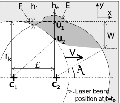
Now let us estimate the period of the intermittent ejection on the kerf side, which corresponds to the striation wavelength. In the following discussion, we restrict ourselves within the velocity range of 2 m/min < V < 6 m/min. In this range, is well defined; the dynamics of side flow is regular, without being perturbed by the central flow as is the case for V < 2 m/min.
In figure 9 is shown the kerf side region seen from the above. At t = t0, the precedent ejection cycle is over, and the kerf profile at the surface almost coincides with the laser beam front (beam centre at C1). After this moment, laser beam proceeds along the x-axis and solid material in the unstable part, the width of which is defined by W, enters the beam area. It is melted very rapidly from the top surface, but not ejected immediately, and accumulation starts. As in the discussion of the instability in the central region, the accumulation continues until the time when the thickness of the melt accumulation reaches , which is given by (13), and then ejection occurs. At that time laser beam centre is at C2 and we can consider that the length of the segment U1U2 in figure 9 as the characteristic thickness of the ejected melt. Using the triangle C1C2U2, the pitch of striations can be determined from the following relation:
2 2 2 k k r r
(15) Using the fact that << rk, one obtains
2
r
k (16) It is shown that striation wavelength is larger than , which defines the pitch of humps in the central part of the kerf front, by a factor of (2rk/)1/2
. Substituting into (16) the theoretical value of = 150 m obtained from the equation (13), is found to be ~500 m. This is more than two times larger than the experimentally obtained wavelength for 2 m/min < V < 6 m/min (~200 m). However, considering the fact that there has already been the overestimation in (about a factor of 2), it can be said that the simple model well predicts the magnitude of .
It is considered that the model shown in the above is only valid for the case where W > . As is
r
k
λ
h
fh
ex
y
F
E
U
1U
2V
W
Laser beam
position at t=t
0+
+
C
1C
2r
k
λ
h
fh
ex
y
F
E
U
1U
2V
W
Laser beam
position at t=t
0+
+
C
1C
2Figure 9. Schematic of melt accumulation process at the top part of the kerf side seen from
evident from the geometry shown in figure 9, if W < , the thickness of melt accumulation is expected to be kept smaller than . This means that the accumulation is too thin to be ejected under the given gas condition. In this work, W decreases with V and it becomes the order of (70 m: experimental value) at V = 5 m/min. This is probably the mechanism of disappearance of unstable region on the side, which was observed around this velocity, at V = 6 m/min.
Whereas the expression (16) predicts that is independent of V, experimental result shows that slightly decreases with V. We consider that two factors, which are not taken into account in (16), may cause this discrepancy.
The first one is temperature dependence of surface tension coefficient , which influences the value of according to the equation (13). As the velocity increases, the kerf width dk (= 2rk) decreases as shown in figure 3. This leads to the increase of the local intensity of laser beam at the kerf side, as is deduced from the intensity distribution in figure 1(b). Whereas the temperature just at the solid-liquid boundary on the kerf side is kept constant at Tm, the temperature gradient (∂T/∂y) in the melt accumulations increases with increasing V. The average temperature in the accumulation is thus elevated, so that should decrease.
The other is the azimuthal melt flow along the semi-circular kerf front. As already mentioned, this kind of flow becomes more important when V and thus increases. This will induce increases of material flow rate into the unstable side region and of temperature in the region by the transport of material from the highest intensity region, both of which tend to decrease . It can be added that with smaller beam spot and higher cutting speed, the lateral flow will become more important.
4.3.2. Surface roughness
Another practical interest of this model is the estimation of surface roughness due to the striations. The roughness may be approximated by sum of the two distances hf and he defined in figure 9:
e f
z h h
R (17) The first term hf corresponds to thickness of the part F of material (figure 9) which is expelled from the laser beam area during the accumulation period and thus is solidified. The height hf can be easily obtained from geometrical relation:
k f
r
h
8
2
(18) which is in the order of 6 m according to the experimental results.The feasibility of the solidification is validated from the following estimation of the time tf, which is necessary to solidify the part F. The solidification results from heat transfer from the liquid part F to the solid part across the sidewall. If the amount of energy transferred exceeds the energy released during the phase transition from liquid to solid, the part is solidified. Thus the time tf can be estimated from
m f s f h L t q
(19) Here we have neglected temperature increase of liquid over Tm. The heat flux q can be written as
y
T
T
K
q
m
0 (20) where y is the characteristic distance of the temperature field along y-axis in the solid side.This distance y is estimated from the fact that the power necessary to heat up the width y of the solid part along each side of the kerf corresponds to the heat conduction loss pl given in the equation (7). That is,
0
2 V yC T T
pl
s ps m (21) Using the equation (7),k r Pe y 7 . 0 2 (22) From (19), (20) and (22), one obtains
7 . 0 2
2
8
Pe
St
t
f
(23) where
m m psL
T
T
C
St
0 (24) is the non-dimensional Stephan number (St ≈ 1.8 for steel). It is estimated that the time tf is about 0.15 ms at V = 3 m/min. This time is much shorter than the accumulation period ta = /V (ta = 4 ms at V = 3 m/min).The second term he in the right hand side of (17) represents the melting of the solid region (part E in figure 9) due to the heat transfer from the melt accumulation. The phenomenon is quite similar to the above solidification, but the great difference is that now the accumulation within the beam area always absorbs laser intensity, so that melting of the solid part persists as long as the accumulation stays at the top or propagates downwards. We suppose that all the energy transferred from the liquid side is spent to erode the solid part, neglecting the dissipation of energy deep into the solid part. Then the eroded thickness he can be estimated from the same discussion as above: m e a
h
L
t
q
(25) Here ta = /V and the heat flux q is the same as in (20). Thus using (20) and (22),
3 . 0 7 . 02
St
Pe
h
e (26) The roughness is finally obtained as 0.7 30. 2 8 Pe St r R k z
(27) The theoretical values predicted from (27) are plotted in figure 5. The experimentally obtained was substituted to (27) in the calculations. The model overestimates the roughness approximately by a factor 3, but it well predicts the decrease of Rz with the increase of V. 4.3.3. Dependence on operating parametersFrom the approximate expression (27), principal influence of operating parameters on Rz is deduced. If we suppose moderate Pe number in the range of 1 < Pe < 10, as in the condition of the present study, the second term of erosion (he) is much larger than the first term of solidification (hf). Using also the expression of in (16),
0.2 0.3
0.3 0.2
0.5 3 . 0 7 . 02
2
k zr
V
St
Pe
St
R
(28)First, is a function of , g and vg, as shown in the equation (13). It decreases with the increase of vg or that of Pin, which raises g. Hence the preparation of appropriate gas condition is an important factor to improve cutting quality, as is a well-known experimental fact. The preceding part (V-0.3rk0.2) represents the dependence on the operating parameters of laser. It suggests that increase of V or decrease of rk will slightly improve the roughness.
Although this work is based on the observation with rather large focal spot (df = 1.7 mm), we have reached the general expressions of , and Rz. In order to verify applicability of the model, we are now investigating dependence of these quality parameters on the operating parameters. Preliminary results with a focal spot df = 0.56 mm and with similar gas condition as in this study shows that the wavelength is about 120 m in the intermediate velocity range (V = 4 m/min). The value is smaller than those obtained in this work (~200 m) by a factor of 1.7, which is consistent with the rk
1/2
dependence of predicted by the model. More experiments will be conducted for complete verification of the model.
5. Conclusion
We have investigated the hydrodynamics in the top part of kerf front during the laser cutting of 3 mm thick mild steel with inert gas of nitrogen. The 8 kW disk laser beam was focused to the diameter of 1.7 mm with the top-hat intensity distribution. We adopted the large focus diameter in order to better visualise phenomena around the kerf front and to reveal the mechanism of the striation initiation.
The melt flow exhibited strong instabilities. The feature can be classified into several regimes depending on the cutting velocity. For 1 m/min < V < 2 m/min, the whole part of the kerf shows discontinuities. The existence of humps, which slide down in the central part of the kerf, was firstly confirmed in laser cutting process. For 2 m/min < V < 6 m/min, the central region becomes stable, but the kerf side region is still discontinuous. The coexistence of stability and instability is an important feature, which has not been discussed in the past. In this range of V, the side flow is characterised by periodic generation of accumulations at the top part and their displacement downwards. It was revealed for the first time that this periodic process is the origin of regular vertical striations left on the kerf side. And finally, the unstable side flow is overwhelmed by the stable central flow at V = 6 m/min.
We discussed the mechanism of the instabilities in the central and side flows, focusing on two physical processes: the instability in thermal dynamics, which is related to localised melting, and the instability in hydrodynamics, which is governed by the force balance between gas force and resistant surface tension force. The localised melting tends to occur in a region where the kerf front wall becomes nearly vertical. In this region melt accumulations are produced periodically. The interval of the accumulation generation is determined by the balance of gas force and surface tension force. The proposed model gives coherent explanation of the instabilities observed both in the central and side regions of the kerf. It also shows reasonable agreement with the experimentally measured hump period, striation wavelength and surface roughness.
Considering simplicity and scalability of the expressions obtained, the authors expect that the model presented in this study will be validated for a wide range of operating parameters and hopefully be utilised to develop innovative processes.
References:
rechnergestützten Prozeßoptimierung Ph. D. Thesis RWTH Aachen (Aachen: Verlag Shaker) [2] Duan J, Man H C and Yue T M 2001 Modelling the laser fusion cutting process: I. Mathematical modelling of the cut kerf geometry for laser fusion cutting of thick metal J. Phys. D:Appl. Phys. 34 2127-2134
[3] Mas C, Fabbro R and Gouedard Y 2003 Steady-state laser cutting modelling J. Laser Applications 15 145-152
[4] Himmer T, Pinder T, Morgenthal L and Beyer E 2007 High brightness lasers in cutting applications Proc. 26th Int. Congress on Applications of Lasers & Electro–Optics 87-91
[5] Hilton P A 2009 Cutting Stainless Steel with Disc and CO2 Lasers Proc. 5th Int. Congress on Laser Advanced Materials Processing No. 306
[6] Arata Y, Maruo H, Miyamoto I and Takeuchi S 1979 Dynamic behavior in laser gas cutting of mild steel Trans. JWRI 8 15-26
[7] Kaplan A F H, Wangler O and Schuöcker D 1997 Laser Cutting: Fundamentals of the periodic striations and their on-line detection Lasers in Engineering 6 103-126
[8] Ermolaev G V and Kovalev O B 2009 Simulation of surface profile formation in oxygen laser cutting of mild steel due to combustion cycles J. Phys. D:Appl. Phys. 42 185506
[9] Miyamoto I and Maruo H 1991 The mechanism of laser cutting Welding in the World 29 283-294
[10] Schuöcker D 1986 Dynamic phenomena in laser cutting and cut quality Appl. Phys. B 40 9-14
[11] Schulz W, Kostrykin V, Nießen M, Michel J, Petring D, Kreutz E W and Poprawe R 1999 Dynamics of ripple formation and melt flow in laser beam cutting J. Phys. D:Appl. Phys. 32 1219-1228
[12] Vicanek M, Simon G, Urbassek H M and Decker I 1987 Hydrodynamical instability of melt flow in laser cutting, J. Phys. D:Appl. Phys. 20 140-145
[13] Chen K and Yao L 1999 Striation formation and melt removal in the laser cutting process J. Manufacturing Processes 1 43-53
[14] Kovalenko V S, Romanenko V V, and Oleschuk L M 1987 High Efficient Processes of Laser Material Cutting (Kiev: Technika)
[15] Makashev N K, Asmolov E S, Blinkov V V, Yu Boris A, Buzykin O G, Burmistrov A V, Gryaznov M R and Makarov V A 1992 Gas hydrodynamics of metal cutting by cw laser radiation in a rare gas Sov. J. Quantum Electron. 22 847-852
[16] Makashev N K, Asmolov E S, Blinkov V V, Yu Boris A, Burmistrov A V, Buzykin O G and Makarov V A 1994 Gas-hydro-dynamics of CW laser cutting of metals in inert gas Proc. SPIE
2257 2-9
[17] Golubev V S 2004 Melt removal mechanisms in gas-assisted laser cutting of materials Eprint No. 3 (Shatura: ILIT RAS)
[18] Matsunawa A and Semak V 1997 The simulation of front keyhole wall dynamics during laser welding J. Phys. D:Appl. Phys. 30 798-809
[19] Yudin P and Kovalev O 2007 Visualization of events inside kerfs during laser cutting of fusible metal Proc. 26th Int. Congress on Applications of Lasers & Electro–Optics 772-779 [20] Landau L D and Lifshitz E M 1987 Fluid Mechanics 2nd edition (Oxford, UK: Butterworth-Heinemann) pp 316-320
[21] Kaplan A F H 1996 An analytical model of metal cutting with a laser beam J. Appl. Phys.
79 2198-2208
[22] Semak V and Matsunawa A 1997 The role of recoil pressure in energy balance during laser materials processing J. Phys. D:Appl. Phys. 30 2541-2552
[23] Schulz W, Becker D, Franke J, Kemmerling and Herziger G 1993 Heat conduction losses in laser cutting of metals J. Phys. D:Appl. Phys. 26 1357-1363
[24] Woods K J and Parker R 1999 Two-Color Imaging Pyrometer Temperature Measurements of the Kerf Front During Laser Cutting Proc. 18th Int. Congress on Applications of Lasers &
Electro–Optics 96-105