3-D numerical modeling of the P and SV wave reflections from fractured reservoirs

3-D Numerical Modeling of the P and SV wave reflections

from Fractured Reservoirs

by

Xiang Zhu

Submitted to the Department of

Earth, Atmospheric, and Planetary Sciences

in partial fulfillment of the requirements

for the degree of

Master of Science

at the

MASSACHUSETTS INSTITUTE OF TECHNOLOGY

MASSACHUSETTS

August, 1997

@ 1997

INSTITUTE OF TECHNOLOGY

Signature of Author ... . . . . I ... . . .... .. . . .. . .U - % .. . . .. . . . . . . . . .

Departiient of

4

_{arth, Atmospheric, and Planetary Sciences}

August, 1997

C ertified by ....

,

... ....

... .. ...

Professor M. Nafi Toks~z

irector, Earth Resources Laboratory

Thesis Advisor

Accepted by...

.

Professor Thomas H. Jordan

-~ Department Chair

WIT

3-D Numerical Modeling of the P and SV wave reflections

from Fractured Reservoirs

by

Xiang Zhu

Submitted to the Department of Earth, Atmospheric, and Planetary Sciences on August 1, 1997 in partial fulfillment of the requirements

for the degree of Master of Science

ABSTRACT

We study the P and SV waves reflections from fractured reservoirs using 3-D finite-difference simulations. The fractures induce anisotropy in seismic velocities. Our calculations illus-trate the effects of this fracture-induced anisotropy on the reflection amplitudes. When the fracture density distribution is heterogeneous, this heterogeneity perturbs the reflections. The strength of this perturbation depends on many factors, such as wavelength, hetero-geneity scale, azimuth, and incident angle. We discuss the influence of these factors, and the possible ways to retrieve the heterogeneity distribution information from the reflection data. The results can help in understanding the seismic reflection data and characterizing the fractured reservoirs.

Thesis supervisor: M. Nafi Toksdz Title: Professor of Geophysics

I thank Dr. Nafi Toks6z for his guidance, support and friendship these past two years. I am very impressed by his kindness to people, and feel fortunate to have him as my advisor. It takes a greal deal of intelligence and effort to set up and direct a scientific research lab of this size. His hard work has made the Earth Resources Laboratory a great learning environment from which many students have benefited.

I thank Dr. Zhenya Zhu for having been very supportive both in research and in life.

He has always been there to discuss problems with me, to make suggestions and to provide help.

I thank Feng Shen for working closely with me on this project. Her research insights,

enthusiasm, intelligence and diligence have been very impressive. I had a very good time working with her. We shared difficulties, progress and a lot of laughs along the way. All of

these will certainly be a good memory to keep.

I thank Bertram Nolte for spending so much time reviewing this thesis, correcting many errors so that this thesis is now much more presentable.

I also thank Jie Zhang, Matthias Imhof, Ningya Cheng, Bertram Nolte, William Rodi, Arthur Cheng, Dale Morgan, Ross Hill, John Queen, Rick Gibson and Dan Burns for helping me many times on various research topics. Their broad knowledge in physics, geophysics and mathematics have made the discussions with them very fruitful. I also learned many computer skills from Joe Matarese and Matthias Imhof.

I have also enjoyed the friendship of many other people in this community. They are: Hafiz Alshammery, Sara Brydges, Wei Chen, Chuck Doll, Antonio De Lilla, Maria Perez, Matthijs Haartsen, Liz Henderson, Xiaojun Huang, Elliot Ibie, Mary Krasovec, Oleg Mikhailov, John Olson, Philip Reppert, Franklin Ruiz, Weiqun Shi, Jesus Sierra, Sue Tur-bak, Roger Turpening, Lori Weldon and more. I am grateful for this.

Contents

1 Introduction 7

1.1 O bjective . . . . 7

1.2 Effective Medium Model of fractured reservoirs . . . . 8

1.3 The Com putation . . . . 9

2 Homogeneous Fractured Medium 11 2.1 Reflection Pattern of P-P and P-SV . . . . 11

2.2 Dependence on Fracture Density . . . . 13

2.3 Dependence on v,/v, ratio . . . . 13

3 Fracture Density Heterogeneity 20 3.1 Azimuth dependence . . . . 21

3.2 Scale dependence . . . . 22

3.3 Nonlinear distortion . . . . 23

3.4 Comparison between the P and SV waves . . . . 24

3.5 Characterizing heterogeneity perturbation without using reference model . 24

A Effective Medium Models of Fractured Reservoirs

B 3-D Finite-Difference Modeling 44

B.1 Finite-difference method . . . . 44 B.2 Form ulation . . . . 45 B.3 Stability condition . . . . 48 B.4 The heterogeneous model input to the 3-D finite-difference program . . . . 48

Chapter 1

Introduction

1.1

Objective

A medium containing vertical fractures is anisotropic, which may cause azimuthal variations

in seismic wave reflections. This anisotropic reflection behavior can be used to derive the properties of the fractured medium. To accomplish this, a thorough understanding of the effects of fractures on reflection amplitude is very important.

One way to calculate the reflection amplitudes is to solve the anisotropic Zoeppritz equations analytically (Riiger and Tsvankin, 1995; Thomsen, 1993; Teng, 1996; Li, 1996). Due to the complexity of these equations, approximations are made in deriving explicit solutions, which are based on assumptions of small velocity contrasts, small source-receiver offsets, and weak anisotropy. These solutions also assume that the seismic wavelength is much smaller than the heterogeneity scale at the reflecting horizon. Furthermore, the analytic solutions of the reflections are available only for azimuths normal and parallel to the fracture planes.

In this thesis we use a 3-D elastic finite-difference program to simulate wave propaga-tioned and calculate reflections from fractured reservoirs. The finite-difference calculations

avoid the assumptions of the analytical derivations, therefore provide more realistic solu-tions. They take into account finite geometry (scaled to wavelength), and are capable of dealing with heterogeneous cases and examining the dependence on heterogeneity scale. The calculations cover arbitrary azimuth, therefore give more complete solutions.

1.2

Effective Medium Model of fractured reservoirs

When aligned fractures are introduced into an originally isotropic background medium, the medium becomes anisotropic. It is symmetric around the axis perpendicular to the fractures. This symmetry is known as transverse isotropy (TI). When the fracture planes are vertical, the symmetry axis is horizontal, resulting in the type of anisotropy called horizontal transverse isotropy (HTI).

We compute the effective elastic constants of the HTI model for the fractured reservoirs using the theory developed by Hudson (1980, 1981, 1990) and Hudson et al. (1996a, 1996b). In this theory, the fractures are in the form of penny-shaped cracks, with dimension much smaller than the seismic wavelength. The detailed formulation is in the appendices.

In a HTI medium, the velocities of the P and SV waves (strictly, quasi P and quasi SV waves) are functions of the azimuth

#,

where

#

is defined as the angle between the incident plane and the symmetry axis of the medium (the x axis in this study). When

#

= 900, the

incident plane is parallel to fracture planes, and the particle motions of the P and SV waves are restricted to this plane. In this case, there is no interaction between the waves and the fractures, and the seismic velocities are the same as in the isotropic case. As

#

decreases, particle motions start to intersect the fracture planes, changing the wave velocities. The velocities are nonlinear functions of the azimuth. For weak anisotropy, they can be expanded in Taylor's series, with cos 26 and cos 46 as the lowest terms. In most cases of gas-saturated fractures, the quasi P wave velocity is dominated by the cos 26 term, therefore it decreases monotonically from

#

= 90' to

#

= 00. Its contour displays a near-elliptical pattern. For

value at # = 450.

1.3

The Computation

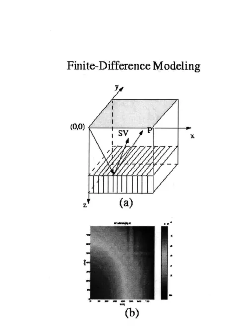
To examine the reflections from fractured media, we build a series of two-layer models. One example is shown in Figure ??a. The upper layer is isotropic for the sake of simplicity. The lower layer is horizontally transversely isotropic, with the x axis as its symmetry axis. This lower layer is formed by introducing vertical fractures into an originally isotropic background medium.

The source at the surface is an explosion. Since the overburden is isotropic, there is only a P wave propagating downward. After the wave reaches the interface, the transmitted energy propagates downward as qP, S1 (fast) and S2 (slow) waves in the HTI layer, while the reflected energy propagates upward in the forms of P, SV and SH waves in the isotropic overburden. We restrict our study to the P and SV waves because the energy of SH wave is small when the reflecting HTI layer is weakly anisotropic. Taking full advantage of 3-D numerical simulation, we record the seismograms over the entire surface, instead of setting up only separated receiver lines. Therefore, we obtain wave reflection amplitudes as

2-D functions of the surface lateral position (x,y). They are conveniently viewed using the

colormaps as shown in Figure ??b.

We use a 3-D parallel staggered-grid anisotropic finite-difference code for the compu-tation. It is second-order accurate in time and fourth-order accurate in space. Higdon's boundary condition is used to absorb waves at the computation model boundaries. The code was originally written by Cheng (1994). We modify it to read in heterogeneous models. A detailed description of our finite-difference calculations is given in the Appendix B.

Finite-Difference Modeling

(0,0)

(a)

wiimOW

(b)

Figure 1-1: The computation model and its reflection amplitude bitmap. (a) The compu-tation model for the 3-D finite-difference program. The receivers are covering the entire surface; (b) The P wave reflection colormap. The x and y axes are lateral receiver positions, and the color represents the reflection magnitude.

Chapter 2

Homogeneous Fractured Medium

We first focus on studying the effects of anisotropy by keeping the fracture density constant, so that the reflecting HTI layers are homogeneous. The results in this section are applicable to the amplitude vs. offset and azimuth (AVOA) because every reflecting point has the same elastic properties.

2.1

Reflection Pattern of P-P and P-SV

The P-P and P-SV reflection coefficients are functions of velocity and density contrasts. The anisotropic behaviors of the wave velocities lead to anisotropic reflection patterns (Mandal et al., 1990). So far, explicit analytic azimuth dependence of the reflection coefficients is not available because the calculations involve complicated tensor rotations. Finite-difference modeling provides a numerical means to examine these azimuthal relations.

Figure 2-1 shows the finite-difference calculations of reflection magnitudes of the P-P and P-SV waves for one of the models described previously. The fractures are filled with gas, and the fracture density is 10%.

The P-P reflection (Figure 2-la) displays a near-elliptical pattern. This pattern can be well explained by the velocity anisotropy. When the P wave is propagating along the fracture orientation (# = 900), its velocity is the same as in the isotropic background. Therefore, the AVO response remains the same as in the isotropic case. Along the other azimuths, the fractures reduce the wave velocities. For gas-saturated fractures, the velocity of quasi P wave is dominated by cos 2# term. It decreases monotonically with the azimuth, displaying near-elliptical pattern. Obviously, this azimuth dependence is passed on to the P-P reflection, and causes a near-elliptical pattern for the reflection. The reflection amplitude at every offset decreases monotonically with the azimuth, reaching its minimum in the fracture normal direction. The reflection pattern is not exactly elliptical because it is also affected by the cos 4# and higher terms in the velocity.

Due to limitation of mesh size, the waves reach the computation boundaries within the time of interest. An absorbing boundary condition is applied to imitate the infinitely-large space. It works well for waves at small incident angles, but generates artificial reflections for waves at large incident angles. They interfere with the signals of interest, and distort the calculations of the magnitudes of waves being measured. This numerical defect causes the straight-line patterns in the colormap. When we plot the reflection curves, this effect is manually removed.

The P-SV reflection (Figure 2-1b) displays a pattern which deviates more from an ellipse. As we know, the P wave velocity variation is dominated by the cos 2# term, while the SV wave velocity has at the lowest order only the cos 4# term. The P-SV reflection coefficient is a function of the P and SV velocity contrast. Therefore, the P-SV reflection is affected by both cos 2# and cos 4# terms. The combination of the effects of these two terms produces such a intermediate pattern in the P-SV reflection colormap.

From our experience with various models, we find that the above patterns hold for gas-saturated fractures in general.

2.2

Dependence on Fracture Density

The fracture density is one of the major factors in determining the anisotropy of the wave velocities, and consequently, the anisotropic behavior of the P and SV wave reflections. The finite-difference calculations clearly reveal the effect of fracture density on reflection.

Figure 2-2 shows the reflection colormaps and curves for models with varying frac-ture density. All models have the same overburden properties. The lower layers are HTI, generated by introducing gas-saturated fractures of various fracture density into the same isotropic background. When the fracture density is zero, the model is isotropic and so are the P and SV reflections. The patterns in the reflection colormaps are circular, showing

no azimuth dependence. The reflection curves at 00, 450 and 90* coincide. As the

frac-ture density increases, the medium becomes anisotropic, and the P and SV reflections are affected by this change. Along the fast wave direction (# = 90'), the reflection curves are

the same as in isotropic case because the waves propagate at the same velocities. But in all other directions, the reflections deviate from the isotropic case. The reflection patterns be-come more elliptical as the fracture density increases. If we define the degree of anisotropy of reflections as the deviation of reflections at

#

= 00 from that at

#

= 900, then it is

approximately proportional to the fracture density.

2.3

Dependence on vp/v, ratio

Even when a large density of fractures is present, the P wave reflection does not necessarily display anisotropic behavior. Sayers and Rickett (1997) show that for some gas sands, there is no visible anisotropy in P wave reflection amplitude within 30 degree incident angle. We find that anisotropy in P wave reflection can be significant for some models. Its visibility

depends on vp/v, ratio.

The effect of v,/v, ratio can be well illustrated by comparing the reflections from Model 1 and Model 2 in Table 2.1. In these two models, the P wave velocities and densities of the

isotropic background materials are the same. They only differ in the S wave velocities. In Model 1, v,/v, = 1.7; in Model 2, v,/v, ~ 1.60. 10% gas-saturated fractures are embedded

into the lower layers. This causes the lower layer P wave velocities in fracture normal direction to decrease by 20%, and S wave velocity by 10% in both models. Finite-difference calculations on the two models give the P wave reflection colormaps and curves as shown in Figure 2-3. For Model 1, the reflection colormap is elliptical, the reflection curves at 00,

450 and 90' azimuths are also well separated. These indicate the medium anisotropy causes

apparent anisotropic behavior in the P wave reflection amplitudes. For Model 2, however, the reflection colormap appears almost circular, with no clearly visible azimuthal variation. The reflection curves at 0', 450 and 900 azimuths coincide. For this model, there is no obvious anisotropic behavior in the P wave reflection amplitudes, even the reflecting layer is anisotropic.

The v,/v, ratio affects reflection anisotropy through Poisson's ratio 0. Poisson's ratio is a major factor determining the P-P reflection. This can be seen by various approximate reflection equations. Among them, the one most explicitly showing its effect is:

Rpp(0) ~ Rp cos2 0 + 2.25A0 sin20

(Hilterman, 1989), where Rp is the normal-incidence reflection coefficient.

Poisson's ratio is related to v,/v, by

}(g)21

(V)21 _

The Poisson's ratio vs. vp/v, plot (Figure 2-4) shows that Poisson's ratio changes faster when v,/v, is closer to 1. In Model 1 and 2, the fractures cause the same amount of percentage decrease in the fracture normal direction wave velocities, but the changes in Poisson's ratios are significantly different (Table 2.1) because of their different v,/v, ratios.

The above results show that the visibility of anisotropy in P wave reflection strongly depends on v,/v, ratio. The models with v,/v, closer to 1 display stronger anisotropy in the reflection amplitudes.

vp vs p vp/vs o- Layer contrast

(m/s) (m/s) (g/cm3) Vp2/vp1 v8 2/v8 1

Model 1 Layer 1 4560 2580 2.67 1.60 0.180

Layer 2 (4 = 90') 4860 3040 2.32 1.60 0.180 1.07 1.07

Layer 2

(#

= 00) 3880 2710 1.43 0.022 0.86 0.96

Layer 2 (azimuth contrast) -20% -11% -11% -116%

Model 2 Layer 1 4560 2680 2.67 1.70 0.235

Layer 2

(#

= 900) 4860 2860 2.32 1.70 0.235 1.07 1.07

Layer 2

(#

= 00) 3850 2570 1.50 0.100 0.84 0.96

Layer 2 (azimuth contrast) -21% -10% -12% -57%

Table 2.1: Elastic properties of the models displaying different degree of reflection anisotropy.

P (Gas,10%) 600 W 1400

200

0 0 200 400

x(m)

x 10-8 2 1.5 1 0.5 200 400

x(m)

-8 x 10 2 1.5 1 600 600 800 SV (Gas, 10%) 600 E400 20C 0 200 400 600

x(m)

x

10

400

x(m)

Figure 2-1: The P and SV wave reflections from a HTI layer. (a) The P wave reflection colormap; (b) The SV wave reflection colormap; (c) The P wave reflection curves (The red, blue and green curves are for 0, 45 and 90 degree azimuths respectively) ; (d) The SV wave

AVO curves.

x

(Isotropic)

0 200 400 600 0.8 0.6 0.4 0.2 0 0 200 400 600

(Gas,5%)

0 200 400 600 0.8 0.6 0.4 0.2 0 0 200 400 800

(Gas,10%)

0 200 400 600 Q 200 400 600

(Gas,15%)

0 200 400 600 0 200 400 600 0 200 400 600 0 200 400 600 x 10 X 10-4 3 0 200 400 600 0 200 400 600 X 10- X 10' 0 200 400 600 0 200 400 600 0 200 400 600 0 200 400 600

Figure 2-2: Reflection of P-P and P-SV waves varying with fracture density. From left to right, each column is for fracture density of 0%(isotropic), 5%, 10% and 15% respectively. The 1st row: reflection colormaps of P waves; The 2nd row: reflection curves of P waves(the maximum offset corresponds to 30 degree incident angle); The 3rd row: reflection colormaps of SV waves; The 4th row: reflection curves of SV waves.

P vz Mode12 (Gas, 10%)

2

600

1.5

E

400

2.5

2

1.5

200

200

400

600

x(m)

200

400

600

800

x(m)

0

200

400

600

x(m)

0

200

400

600

800

x(m)

Figure 2-3: The P wave reflections from models of different v,/v, ratio. Model 1: vp/v, =

1.60; Model 2: v,/v, = 1.70.

600

400

200

0

0

1

0.8

0.6

0.4

0.2

P vz Model1 (Gas, 10%)

x 10

x 10

0 C-Cn

-5

0.15

-

- -- -

---0.1

-0.05

-

---

-

-0

1.4

1.5

1.6

1.7

1.8

1.9

2

VpNs

Chapter 3

Fracture

Density Heterogeneity

In this section we investigate the effects of the fracture density heterogeneity on seismic wave reflections. The reflecting interface is flat. In the fractured layer, the fracture alignment is fixed parallel to the y axis, and the fracture density varies only laterally. Such a layer is modeled as a HTI medium with a fixed symmetry axis and laterally varying strength of anisotropy.

We build a series of test models to examine the effects of the fracture density heterogene-ity on the reflections. These models are still two-layered, with the upper layer homogeneous. In the lower layers, the mean fracture density is 10%, and the variation is within +10%. The fracture density varies as either a smooth cosine function (therefore varying at a fixed spatial frequency), or a certain type of stochastic function. The reflections of the model with homogeneous 10% fracture density yield smooth near-elliptical patterns. We consider the effect of the fracture density heterogeneity as perturbation on this background. We observe this perturbation by comparing the reflections of the heterogeneous fracture density models to the reflections of the mean background, and find the residues. These reflection residues should reveal relations between the model heterogeneity distributions and the reflections.

3.1

Azimuth dependence

As shown in the previous section, the influence of the fractures on the P and SV wave reflec-tions is azimuth dependent. It follows that the effects of the fracture density heterogeneity

also has azimuth dependence.

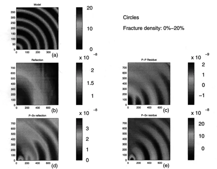
To examine this azimuth dependence, we calculate the reflections for a model where the fracture density is a cosine function of the source-receiver separation. The colormap of this fracture density distribution is shown in Figure 3-la (This figure is actually just a windowed colormap of the model interface, in which only the reflecting area is shown). For this distribution, the variation of the fracture density is at the same spatial frequency at every azimuth. Any azimuthal difference in the reflections is only caused by the variation in the azimuth. We use the value of 160 m as the period of the cosine function. This is about 1.5 wavelength of the P wave. This distribution forms circular pattern around the source in the colormap.

The P wave reflection colormap of this model is shown in Figure 3-1b. It displays near-elliptical pattern, similar to that of the homogeneous model with 10% fracture den-sity. To see the perturbation due to the fracture density heterogeneity, we subtract the reflection for the homogeneous 10% fractured medium from the reflection of this heteroge-neous model. This residue is shown in Figure 3-1c. We find that in the fracture normal direction (# = 00), the reflection is strongly perturbed by the model heterogeneity, and its

residue clearly recovers the model circular rings. As

#

increases, the perturbation of the model heterogeneity decreases, and the rings smear out. In the fracture orientation direc-tion (# = 90'), the rings disappear. This test model demonstrates that the perturbation

3.2

Scale dependence

In heterogeneous media, the geometric scale of heterogeneity relative to wavelength plays an important role in determining the effective values of the physical properties. Mukerji et al.

(1995) found that the velocity increases with decreasing ratio of wavelength to correlation

length. Here the reflection coefficients are also scale-dependent. In the case where the heterogeneity scale is much larger than wavelength, the waves are thin beams sampling the reflecting interface at high resolution. The reflection coefficients are functions of only local elastic constants. When the heterogeneity scale is close to the wavelength, the reflections occur in an area relatively large compared to the wavelength. The reflection from any point is interfering with the reflections from neighboring points, and the wavefront is sensing the average of the elastic constants in the area. The rapid spatial variation is smoothed, as if it were passed through a low-pass filter. When the heterogeneity scale is much smaller than the wavelength, the wave cannot sense the spatial variations, and the reflecting interface is effectively homogeneous.

Figure 3-3 shows the P wave reflection residues for models of different heterogeneity scale. The model heterogeneity distributions follow similar cosine functions, but with vary-ing spatial period. This varyvary-ing period gives models different spatial heterogeneity scale. We find that, for the spatial periods above 1.5 wavelength, the heterogeneous distribution are well sensed by the reflections; below that, the reflection fluctuations due to heterogene-ity is small because of the averaging effect; when the spatial period is below 1 wavelength, the reflection only "sees" an homogeneous interface effectively. One wavelength is roughly the threshold for determining whether the heterogeneity is observable in the reflection am-plitude.

3.3

Nonlinear distortion

Although the reflection residue colormaps form images of the fracture density distribution, the relation between the reflection residue and the (offset,azimuth) coordinates is nonlinear. This nonlinearity distorts the image. The fractures affect the wave particle motions normal to the fracture planes. The fraction of wave energy in particle motions normal to the fractures increases with increasing offset, and decreases with increasing azimuth. These

factors cause nonlinear weighting in the reflection residues.

Figure 3-4 and Figure 3-6 show how straight-line patterns are distorted. They are the re-sults for two models in which the fracture density distributions are 10%+10% cos(27rx/160m) and 10% + 10% cos(27ry/160m). These distributions yield patterns of straight lines parallel

and normal to the fracture planes (Figure 3-4a and Figure 3-6a). The reflection residues of both P and SV waves recover the model straight-line patterns, but with some distortion. The model heterogeneity distribution is better recovered for large offset and small azimuth.

In reality the heterogeneity distribution seldom follows regular patterns such as those we have shown. Therefore, we also test more realistic models built with stochastic functions of the fracture density distribution. Figure 3-8a shows a stochastic model where the fracture density heterogeneity distribution takes the form of a von Ki'rmain function. The correlation lengths are 300 m in both the x and y directions. Figure 3-10a is a similar model with correlation lengths at 100 m in x and 300 m in y. As in the other models, the mean fracture density is 10%, with perturbations of ±10%. For these irregular patterns, we see the reflection residues of P and SV waves do show correlation between the large scale heterogeneous areas of model and the reflection. The model images, however, are severely distorted due to the reflection nonlinear dependence on the incident and the azimuthal angles.

3.4

Comparison between the P and SV waves

For every model, the P-SV reflection is much more sensitive than that of the P-P wave. The P-SV reflection colormap is strongly perturbed by the same heterogeneity distribution. After removing the reflection of the homogeneous background, the residue forms a clearer image of the model heterogeneity pattern. The relative scale of residue is also much lager than that of the P-P wave. This is explained by the greater sensitivity of shear waves to the presence of fractures. The wavelength of the SV wave is smaller than that of the P wave, which also contributes to the better resolution.

3.5

Characterizing heterogeneity perturbation without using

reference model

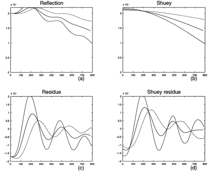
Without using the reflection of the homogeneous fracture density model as a reference, the heterogeneity perturbation can also be determined by using Shuey's equation for P waves along any receiver line. For example, Figure 3-5b is the plots of P wave reflection in Shuey's

two-term approximation (i.e., A + B sin2 6) at

#

= 00, 450 and 90', with A and B

deter-mined by fitting the model reflection curves to Shuey's equation. The reflection residues obtained by subtracting the Shuey curves from the model results also provide heterogeneity information (Figure 3-5d). By doing this, we assume that the best-fit Shuey curves are the reflections of the homogeneous background. Since no homogeneous background reflection is available for processing real data from the field, using Shuey's equation as a reference is a realistic way to obtain the heterogeneity estimates. From the homogeneous case we find that the reflection curves match Shuey's equation very well up to the incident angle of

25 degrees. For higher angles, the deviation becomes significant because Shuey's equation

ignores higher order terms. The reflection residue results (Figure 3-5d) are distorted by this mismatch beyond 25 degrees. For better match at large incident angles, more accurate analytic equations should be used.

Shuey's equation is one-dimensional, and is applicable only to individual receiver lines. There is no explicit analytical equation to be used on 2-D data. Because the heterogeneity perturbation is at high spatial frequencies, and the homogeneous background reflection is at low spatial frequencies, the heterogeneity information may also be retrieved by filtering. This technique can be applied to 2-D reflection data.

Model 0 100 200 300 Reflection 0 200 400 600

(b)

P-Sv reflection

20

10

0

X 10

2

1.5

1

x

Circles

Fracture density: 0%-20%

P-P Residue 0 200 400 600

(c)

P-Sv residue 0 200 400 600

(d)

0 200 400 _600(,)

Figure 3-1: Reflection from a heterogeneous model (circular pattern). (a) The colormap of fracture density in the model reflecting area; (b) Reflection colormap of P wave; (c) P wave reflection residue (homogeneous background removed); (d) Reflection colormap of SV wave; (e) Reflection residue of SV wave.

x 10

2

1

0

-1

x 10

20

10

0

x10

Reflection

x 10.

Shuey

400 500 600 700 800

(a)

Residue

x 10. 0 100 200 300 400 500 600 700 (c)

Shuey residue

x 10. 0 100 200 300 400 500 600 700 800

(d)

Figure 3-2: Shuey fitting for a heterogeneous model (circular pattern). (a) Reflection curves of P wave; (b) Reflection curves fitted into Shuey's equation; (c) Reflection curves residues;

(d) Reflection curve residues after removing Shuey's curve.

x 10- AVO 2 0 -2 . . . OA 1( 200 400 600 800 2 0 -2 .< 10. 200 400 60 80

60m

80m

1OOm

120m

160m

200m

Figure 3-3: The reflection residue for models of circular pattern fracture density distribution. The period of spatial variations are 60, 80, 100, 120, 160, 200 m respectively. The wavelength is 100 m. AVOA 0 500 0 200 0 200 0 200

20

10

0

20

10

0

20

10

20

10

0

20

10

0

20

10

0

600 400 200 0 600 400 200 0 600 400 200 0 600 400 200 0 600 400 200 0 600 400 200 0 0 500 0 500 0 500

%io.

200 400 600 800 q10 200 400 600 800 qki1- 2 4 - 60 8-0 200 400 600 800 0 200 0 200 0 500 0 200 0 500

Model 0 100 200 300

(a)

Reflection 0 200 400 600

(b)

P-Sv reflection 0 200 400 600 (d)

Vertical-lines

Fracture density: 0%-20%

P-P Residue 2

1.5

0 200 400 600

(c)

P-Sv residue 0 200 400 ₆₀₀

_(e)

Figure 3-4: Reflection from a heterogeneous model (vertical-lines pattern). (a) The col-ormap of fracture density in the model reflecting area; (b) Reflection colcol-ormap of P wave; (c) P wave reflection residue (homogeneous background removed); (d) Reflection colormap of SV wave; (e) Reflection residue of SV wave.

x 10

-10

5

0

5

x 10

5

0

-5

Reflection

x 10-' 0 100 200 300 400 500 600 700 800

(a)

Residue

x 10-' 0 100 200 300 400 500 600 700 800

(c)

Shuey

x 10-0 100 200 300 400 500 600 700 800

(b)

Shuey residue

x 10. 0 100 200 300 400 500 600 700 800

(d)

Figure 3-5: Shuey fitting for a heterogeneous model (vertical-lines pattern). (a) Reflection curves of P wave; (b) Reflection curves fitted into Shuey's equation; (c) Reflection curves residues; (d) Reflection curve residues after removing Shuey's curve.

Model 0 100 200 ₃₀₀

(a)

Reflection 0 200 400 6o0 (b) P-Sv reflection 0 200 40 _{W (d)}

20

10

0

-8

X 10

2

1

x 10

3

2

1

n

Horizontal-lines

Fracture density: 0%-20%

P-P Residue 0 200 ₄₀₀ 600 (C) P-Sv residue 0 200 400 800

(e)j

al

Figure 3-6: Reflection from a heterogeneous model (horizontal-lines pattern). (a) The colormap of fracture density in the model reflecting area; (b) Reflection colormap of P wave; (c) P wave reflection residue (homogeneous background removed); (d) Reflection colormap of SV wave; (e) Reflection residue of SV wave.

-10

x 10

2 0 2 .4

6

8

-9

X 10

4

2

0 -2 -4

Reflection

x10.

x 10.' 0 100 200 300 400 500 600 700 800

(a)

10.

Residue

0.5 0 -0.5 -0.5 0 100 200 300 400 500 600 700 800 (c)

Shuey

0 100 200 300 400 500 600 700 800

(b)

Shuey residue

x 10. 0 100 200 300 400 500 600 700 800

(d)

Figure 3-7: Shuey fitting for a heterogeneous model (horizontal-lines pattern). (a) Reflection curves of P wave; (b) Reflection curves fitted into Shuey's equation; (c) Reflection curves residues; (d) Reflection curve residues after removing Shuey's curve.

Model 0 100 200 300 _(a) Reflecaon 0 200 400 600

(b)

P-Sv reflection

20

10

0

-8

X 10

2 1.5

1

x

Random3X3

Fracture density: 0%-20%

P-P Residue 0 200 400 600

(c)

P-Sv residue 0 200 400 _{o (d)8} 0 200 400 6o

Figure 3-8: Reflection from a heterogeneous model (von Kirman, 3X3). (a) The colormap of fracture density in the model reflecting area; (b) Reflection colormap of P wave; (c) P wave reflection residue (homogeneous background removed); (d) Reflection colormap of SV wave; (e) Reflection residue of SV wave.

X 10

2

1

0

-1

x

5 0 -5

Reflection

01 0 100 200 300 400 500 600 700

(a)

0.5 F 0 100 200 300 400 500 600 700 800

(b)

Residue

x 10* x 10.

Shuey residue

0 100 200 300 400 500 600 700

(c)

0 100 200 300 400 500 600 700 800

(d)

Figure 3-9: Shuey fitting for a heterogeneous model (von Kirman, curves of P wave; (b) Reflection curves fitted into Shuey's equation; residues; (d) Reflection curve residues after removing Shuey's curve.

3X3). (a) Reflection

(c) Reflection curves

Model 20 0 100 200 30

(a)

Reflection 0 200 400 600 (b) P-Sv reflection 0 200 400 600 (d)

Random 1 X3

10

Fracture density: 0%-20%

S0

-8

X

10

_{P-P Residue}

1.5

0 200 400 600 P-Sv residue

x 10

3

2

1

0

0 200 400 00

Figure 3-10: Reflection from a heterogeneous model (von Kirmain, 1X3). (a) The colormap of fracture density in the model reflecting area; (b) Reflection colormap of P wave; (c) P wave reflection residue (homogeneous background removed); (d) Reflection colormap of SV wave; (e) Reflection residue of SV wave.

x 10

0

-5

-10

-15

X 10

8

6

4

2

0

-2

Reflection

x10.

x 10* 0 100 200 300 400 500 600 700 800

(a)

Shuey

0 100 200 300 400 500 600 700 800

(b)

Residue

x 10. x 10.

Shuey residue

0 100 200 300 400 500 600 700 (C) 0 100 200 300 400 500 600 700 800

(d)

Figure 3-11: Shuey fitting for a heterogeneous model (von Kirman, curves of P wave; (b) Reflection curves fitted into Shuey's equation; residues; (d) Reflection curve residues after removing Shuey's curve.

1X3). (a) Reflection (c) Reflection curves

Chapter 4

Conclusions

We used 3-D finite-difference modeling to simulate P-P and P-SV reflections from fractured reservoirs. Using these synthetic reflection data, we examined the effects of fracture-induced anisotropy and fracture density heterogeneity on the wave reflections, and their variations with the fracture and background properties. We derived the following conclusions:

The finite-difference calculations verify that fractures cause azimuthal variation in the P and SV wave reflections. The azimuthal variations of the reflections are approximately proportional to the fracture density. The effect of fractures is maximum in the fracture normal direction, and minimum in the fracture alignment direction.

The visibility of anisotropy of reflection depends on the v,/v, ratio; The layers with vp/v, closer to 1 display stronger anisotropy in the reflection amplitudes.

The fracture density heterogeneity perturbs the P and SV wave reflections. The re-flection residues due to fracture density heterogeneity yield distorted images of the model fracture density distribution. The P-SV reflection residue forms a better image that that of the P-P reflection residue.

below a wavelength.

For processing field data, the heterogeneity estimates can be obtained by fitting the data with approximate analytic reflection equations (Shuey's equation, or more accurate ones).

References

Banik, N. C., 1987, An effective anisotropy parameter n transversely isotropic media: Geo-physics, 52, 1654-1664.

Cheng, N., 1994, Borehole Wave Propagation in Isotropic and Anisotropic Media: Three-Dimensional Finite Difference Approach, Ph.D. thesis, Earth Resources Lab, MIT, Cam-bridge, MA

Hilterman, F., 1989, Is AVO the seismic signature of rock properties?: SEG Expanded Abstracts, 59, 559.

Hudson, J. A., 1981, Wave speeds and attenuation of elastic waves in material containing cracks: Geophys. J. Roy. Astr. Soc., 64, 133-150.

Hudson, J. A., 1990, Overall elastic properties of isotropic materials with arbitrary distri-bution of circular cracks: Geophys. J. Int., 102, 465-469.

Hudson, J. A., Liu, E., and Crampin, S., 1996a, Transmission properties of a plane fault: Geophys. J. Int., 125, No.2, 559-566.

Hudson, J. A., Liu, E., and Crampin, S., 1996b, The mechanical properties of materials with interconnected cracks and pores: Geophys. J. Int., 124, 105-112.

Mueller, M. C., 1991, Prediction of lateral variability in fracture intensity using multicompo-nent shear-wave surface seismic as a precursor to horizontal drilling in the Austin Chalk: Geophys. J. Int., 1991, 409-415.

Mukerji, T., Mavko, G., Mujica, D., and Lucet, N., 1995, Scale-dependent seismic velocity in heterogeneous media: Geophysics, 60, 1222-1233.

Li, X., Kiihnel, T. and MacBech, C., 1996, Mixed mode AVO response in fractured media:

SEG Expanded Abstracts, 66, 1822-1825.

Mandal, B. and M. N. Toksdz, 1990, Computation of complete waveforms in general anisotropic media - Results from an explosion source in anisotropic medium: Geophys.

Riiger, A., Tsvankin, I., 1995, Azimuthal variation of AVO response for fractured reservoirs:

SEG Expanded Abstracts, 65, 1103

Sayers, C. M., Kachanov, M., 1995, Microcrack-induced elastic wave anisotropy of brittle rocks: J. Geophys. Res., 100, 4149-4156.

Sayers, C. M., Rickett, 1997, J. E., Azimuthal variation in AVO response for fractured gas sands: Geophysical Prospecting, 45, 165-182.

Schoenberg, M., and Douma, J., 1988, Elastic wave propagation in media with parallel fractures and aligned cracks: Geophys. Prosp., 36, 571-589.

Schoenberg, M., Sayers, C. M., 1995, Seismic anisotropy of fractured rock: Geophysics, 60, 204-211.

Teng, L., Mavko, G., 1996, Fracture signatures on P-wave AVOZ: SEG Expanded Abstracts,

66, 1818-1821.

Thomsen, L., 1993, Weak anisotropic reflections: Offset-dependent reflectivity - Theory and practice of AVO analysis, 103-111.

Virieux, J., 1984, SH-wave propagation in heterogeneous media: velocity-stress finite-difference method: Geophysics, 49, 1933-1957.

Appendix A

Effective Medium Models of

Fractured Reservoirs

In the presence of fractures, the average strain e can be written as

eig = (sjk + sI)jUkI (A.1)

where a is the average stress tensor, sk is the compliance tensor in the absence of frac-tures, and s -kl is the excess compliance tensor induced by fractures (Sayers and Kachanov,

1995; Schoenberg and Sayers, 1995).

The excess strain can be computed by

1 N[

szjklikl = E ([uijnj -+ [ujlni)dS

2Vr=1 'r

(A.2)

where [us] is the ith component of the displacement discontinuity on S, ni is the ith component of the fracture normal, and Nf is the number of the fractures in the area S.

Assuming that fracture interactions may be neglected so that [uI) is determined by o-i, and all fractures in V are identical with each having the same normal n and a surface area

S, then a linear slip boundary condition is given by

[Uij = Zij₃ jknk (A.3)

where Zij is the fracture system compliance tensor.

Assuming the fracture is invariant with respect to rotation about the axis along the fracture normal, then

Zij = ZTSjo + (ZN - ZT)ninj (A.4)

where ZN and ZT are normal and tangential compliances of the fractures (Schoenberg and Sayers, 1995).

Combining the above equations, and define the fracture density as el = N S we have

jkl = [ZT(6 kninj + 6

jknini + 6i1nknj + 6 inkni) + 4(ZN - ZT)rningnni (A.5)

We follow Hudson et al. (1996a) and Schoenberg and Douma (1988) to model the aligned fractures. The compliance tensors can be written as

3

ZN = 7a U3 3 (A.7)

p

where -y is the number of elementary fractures per area, a is the average radius of the circular cracks. For dry cracks, Hudson (1981) gives

16 A +2pi

U11 = 16A+2_{3 3A+ 4p-}1L (A.8)

U33 = 4 A+2 (A.9)

3 A+p

Define the crack density as y = el-ya3

, and insert Eq. A.6 and A.7 to Eq. A.5, we have

STjk = 4 [U11(6iknin + 6jknini + 6 inknj + 6

Appendix B

3-D Finite-Difference Modeling

B.1

Finite-difference method

Finite-difference method is a popular way to solve the wave equation and other partial dif-ferential equations. It has been intensively used to simulate wave propagation and reflection after the progress made in absorbing-boundary conditions and staggered-grid discretization in the seventies.

We use a 3-D finite-difference code developed at Earth Resources Laboratory (ERL) (Cheng, 1994). The program uses a staggered-grid discretization scheme (Madariaga,1976; Virieux, 1984). Its advantages are: it is stable for any Poisson's ratio; the grid dispersion and anisotropy are small and insensitive to Poisson's ratio. The absorbing boundary condition is Higdon type (Higdon, 1986, 1987, 1990). It works well at the boundary with lateral heterogeneity. It is easy to implement, and does not require special treatment at the corners of the grid. The program is capable of dealing with models of orthorhombic anisotropy. It is the most general case without normal stress and shear strain coupling. The isotropic and TI models are its special subclasses. For many geophysical applications, lower symmetries need not be considered. The program is implemented on the nCUBE parallel computer

at ERL. Parallel implementation greatly increases the computation power and makes it realistic to simulate wave propagations in 3-D models.

B.2

Formulation

The equation of motion in an elastic medium is:

PtUi = rijj (B.1)

where p is the density, ui is the displacement vector, and rij is the stress tensor. The comma between the subscripts denotes spatial derivative. The equation is in Einstein's notation, which implicitly implies summation over all repeated subscripts.

The generalized form of Hooke's law is

rij= CijklEkl _(B.2)

where Cijkl _{is the fourth-order elastic stiffness tensor, and the strain tensor is defined as:}

E=

(ui,j

_{+ Uj,i)}

If we replace the strain tensor by the strain vector

Exx Eyy E = EZZ 2 6yz 2exz \2exy (B.3) (B.4)

and replace the stress tensor by the stress vector 7 -xx Tyy

T =

TZZ (B.5) Tyz TxY

then the fourth-order elastic stiffness tensor can be replaced by a 6 x 6 symmetric stiffness matrix because of the symmetry properties of the tensor.

C=

C1i C12 C22 C13 C₂3 C_{3 3} c16 C26 C_{3 6} C46 C56 C_{6 6}

\

symmetric

(B.6)

where the subscripts 1,2,3 denote xx,yyzz, and or zx, xy or yx, respectively.

the subscripts 4,5,6 denote yz or zy, xz

The generalized Hooke's law in matrix form is:

T=CE

For an orthorhombic model, the stiffness matrix is

C_{1 1} C12 C_{2 2} C13 C23 C33

K

symmetric

0 0 0 0 0 0 0 0

C55

0

C66 (B.7) (B.8)

Vertically aligned fractures form models of vertical, transverse isotropy. This symmetry is a special case of orthorhombic symmetry. Assuming the x-axis is the symmetry axis, the corresponding stiffness matrix is

C11 C12 C12 0 0 0

C22 C23 0 0 0

c22 0 0 0

where c23 = c22 - 2c₄₄.

A staggered-grid scheme calculates velocity and stress using Equations (B.1) and (B.7).

For an orthorhombic medium, they can be written as

Bvx p

at

=

Pavy

at

at

and

at

atxx

at

at

aTXY

at

atz

at

o-ryz

at

ax±

a7y

ay

aTXY

aTYY

ax

+ay

aTxz

aTyz

ax+

ay

Cv1p

=cii -

+

C12 ay

az

az

+

aT

oz

(B.10) + C13 Bz C12ax + C22

+

C₂₃

p

ax

ay

49z

= C₁3

ax

=

c44(-ay

av

= 55(y = C66(

az

9z

C23 y

ay

+ aV)

ax

+

vz

ax

+ovz

ay

+ C33

49z

(B.11)

C44

0

c55 0

\

symmetric (B.9)

C55

/

These equations are discretized on a staggered grid in coordinates (mAx,nAy,kAz) at time iAt. The second-order forward finite-difference operator in time Dt is

Dtf ,n,k _ mfnA,k - m,n,k (B.12)

and the fourth-order forward finite-difference operators in space D2, DY and Dz are Dxff,,, = f1nm1,n,k - fm,n,k + ₇₇2 -AX AX DyfI,,k = 71 fm,n+1,k - fm,n,k + 72 fm,n+2,k - Am,n-1,k (B.13) Ay Ay Dzf ,,k = 771 k - ± f,n,k+2 - m -Az A z 9

where 771 = | and 772 = - are the coefficients of the fourth-order finite-difference

approx-imation to the first-order derivative.

B.3

Stability condition

Assume Ax = Ay = Az = A, the stability condition for 3-D is

At

<

A(B.14)

V"3(

711

I

±

ImIj)

(.

where a is the P wave velocity, and Y1,2 are differential operator coefficients. For the

fourth order finite-difference approximation, q1 = 2, and 772 = -1

B.4

The heterogeneous model input to the 3-D finite-difference

program

We modified Cheng's 3-D finite-difference program for wave simulation in heterogeneous media. The original program only takes models composed of a few homogeneous blocks of

various shapes. We added an input option (No. 9) into the program. With this option, the program can read in a 2-D bitmap of laterally varying heterogeneous model. For our purpose of studying lateral fracture density variation, this is sufficient since the fractures are vertical.

Option No. 9 expects two layers. The first layer is homogeneous, and the second layer is heterogeneous. For this heterogeneous layer, there are many different fracture densities present, and therefore many different elastic stiffness matrices to specify. These matrices are in the file <model-name>.index2elasticconsts. The heterogeneous fracture density distribution is in the file <model-name>.pos2index.

An example of model input file using option No. 9 is as follows.

160, 160, 170 9 0 202 t5.index2elasticconsts t54.pos2index 2.67 2.32 2 130,170 8000.0, 0.8 0700 0.045 40,40, 40 40,40, 40 0 0, 10, 0 1, 10, 10, 1 t54.00sg \model size: mm nn kk \model: 0 H 1 BH 2 Ly 3 CO 4 RAN \Free surface: 1 yes 0 absorbing \number of stiffness matrices \postfix of elastic consts file \cos circles, model index table file

\density of block 2--102, in g/cm^3 \ nlayer

\ layer(i)

\dx(mm), dt(ms)

\total time step

\source center frequency (kHz) \receiver position: irx,iry,irz \source position: isx,isy,isz

\type: 0-P,1-Fx,2-Fy,3-Fz \graphyic: 1- yes, imageskip,iwrit \seisgram: iskip, ntrace,idd,direc

\seisgram output file

The input lines in the file specific to option No. 9. are:

9 Line 2: specifying that the program is reading input model following option 9. e Line 4: number of different elastic stiffness matrices.

" _{Line 5: the file containing elastic constants for every fracture density.}

" Line 6: the file containing the fracture density distribution.

* Line 7: the density of the two layers.

A section of the elastic constants file t5.index2elasticconsts and a section of the fracture

density distribution file t54.pos2index are shown below as examples: t5.index2elasticconsts: 55.54 0.0000 0.0000 0.0000 54.7975 0.0000 0.0000 0.0000 54.7927 0.0000 0.0000 0.0000 23.83 0.0000 0.0000 23.9055 0.0000 0.0000 23.9055 0.0000 0.0000 23.83 0.0000 23.9055 0.0000 23.8457 0.0000 -- fracture density -- c11 -- c21 c22 -- c31... c33 -- c41... c44 -- c51.. .c55 23.83 -- c6... c66 23.9055 23.8457

In this file, every 7 lines is one set of data for one value of fracture density. The first line is the fracture density (dimensionless). The remaining 6 lines are the elastic stiffnesses in units of 103kg/m/s 2. The first set is for the homogeneous upper layer. The remaining 201 sets are for the second layer.

0.000 55.54 7.87 7.87 0.0000 0.0000 0.0000 0.000 54.7975 6.9864 6.9864 0.0000 0.0000 0.0000 0.001 54.5021 6.9488 6.9488 0.0000 0.0000 0.0000 55.54 7.87 0.0000 0.0000 0.0000 54.7975 6.9864 0.0000 0.0000 0.0000 54.7927 6.9816 0.0000 0.0000 0.0000

t54.pos2index: 9.8 10.9 11.9 12.8 13.6 14.3 14.7 15.0 15.0 14.8 x y fracture density

(M)

The first two columns are the grid point indices. The third column is the fracture density in percentage.