is an open access repository that collects the work of Arts et Métiers Institute of
Technology researchers and makes it freely available over the web where possible.
This is an author-deposited version published in: https://sam.ensam.eu Handle ID: .http://hdl.handle.net/10985/15375
To cite this version :
Paola CINNELLA, Karim GRIMICH, Alain LERAT, P. Y. OUTTIER - Recent Progress in High-Order Residual-Based Compact Schemes for Compressible Flow Simulations: Toward Scale-Resolving Simulations and Complex Geometries - 2015
Any correspondence concerning this service should be sent to the repository Administrator : [email protected]
Compact schemes for compressible flow
simulations : toward scale-resolving simulations
and complex geometries
P. Cinnella, C. Content, K. Grimich, A. Lerat, P.Y. Outtier
Laboratoire DynFluid, Arts et M´etiers ParisTech, 151 bd. de l’Hˆopital, 75013, Paris,
France [email protected]
Abstract. Recent developments about the extension of high-order
Residual-Based Compact schemes to unsteady flows and complex configurations are discussed, with application to scale-resolving simulations and com-plex turbomachinery flows.
Keywords: High-order, Residual-Based Compact Scheme, Scale-Resolving,
Overset grids
1
Introduction
This paper summarizes recent developments of a family of high-order Residual-Based Compact (RBC) schemes, initially proposed by [1, 2]. Differently from standard numerical schemes that approximate space derivatives independently in each space direction, RBC schemes seek for a compact approximation of the complete residual r, i.e. the sum of all derivatives in the governing equations. Because of this feature, RBC schemes belong to the group of so-called genuinely multidimensional schemes such as the fluctuation splitting schemes or the Resid-ual Distribution (RD) schemes (see, e.g. [3, 4]).
Major developments described in the following focus on the extension of RBC schemes to unsteady flows and to complex geometries. Selected applications, including two application challenges among those considered in the IDIHOM project, are presented to assess the capabilities of the schemes, specifically for scale-resolving simulations and complex transonic turbomachinery flows.
2
RBC Schemes
In this Section, we recall the design principles of RBC approximations of the space derivatives for a hyperbolic system of conservation laws. For the sake of brevity, we will focus on two-dimensional problems, but there is no restriction to extend the analysis to multi-dimensional hyperbolic problems. At this stage, we treat time derivatives exactly, i.e. we focus on semi-discrete approximations in space.
2.1 High-order RBC schemes
Let us consider the hyperbolic system of conservation laws:
wt+ fx+ gy = 0 onR2× R+ (1)
with initial conditions
w(x, y, 0) = w0(x, y)
where t is the time, x and y are Cartesian space coordinates, w is the state vector and f = f (w), g = g(w) are flux components depending smoothly on w. The Jacobian matrices of the flux are denoted A = df /dw and B = dg/dw. System (1) is approximated in space on a uniform mesh (xj= jδx, yk = kδy), with steps
δx and δy of the same order of magnitude, sayO(h), using the basic difference
and average operators: (δ1v)j+1 2,k= vj+1,k− vj,k (δ2v)j,k+12 = vj,k+1− vj,k (µ1v)j+1 2,k= 1 2(vj+1,k+ vj,k) (µ2v)j,k+12 = 1 2(vj,k+1+ vj,k)
where j and k are integers or half integers.
A residual-based scheme is expressed in terms of approximations of the exact residual:
r := wt+ fx+ gy (2)
More precisely, such a scheme is of the form:
( ˜r0)j,k= ˜dj,k (3)
where ˜r0 is a space-centered approximation of r called the main residual and ˜d
is a residual-based dissipation term defined as: ˜
dj,k=
1
2[δ1(Φ1r˜1) + δ2(Φ2r˜2)]j,k (4) where ˜r1 and ˜r2, respectively defined at j + 12, k and j, k + 12, are also
space-centered approximations of r called the mid-point residuals, and Φ1, Φ2 are
numerical viscosity matrices. These matrices depend only on the eigensystems of the Jacobian matrices A and B and on the steps δx and δy. They are designed once for all [5] and use no tuning parameters nor limiters. Since the matrices Φ1
and Φ2remainO(1) as δx and δy tend to zero, the dissipation ˜d represents, to the
leading order, a numerical approximation of the second-order partial differential term:
d =δx
2 (Φ1r)x+
δy
2 (Φ2r)y (5)
This leading term of the expansion, that is only first order accurate, vanishes for an exact solution (r = 0), so that ˜d is actually consistent with a high-order
In the following, the residuals are discretized by using compact formulae such that: ( ˜r0)j,k = rj,k+O(h2p) ( ˜r1)j+1 2,k= rj+12,k+O(h 2p−2) ( ˜r2)j,k+1 2 = rj,k+ 1 2 +O(h 2p−2). with p≥ 2.
Thus, the dissipation term (4) satisfies: ˜
dj,k= dj,k+O(h2p−1)
and the truncation error of the semi-discrete scheme (3) is
εj,k= rj,k+O(h2p)− dj,k+O(h2p−1).
Since the exact residual r and the leading term d of the residual-based dissipation (5) are null for an exact unsteady solution, we finally obtain:
εj,k=O(h2p−1). (6)
In other terms, approximating the main residual at order 2p and the mid-point residuals at order 2p− 2 leads to a Residual-Based Compact scheme of order
q = 2p− 1. Such a scheme is called RBCq. In the following, we focus on schemes
using 5× 5-point stencils at most, which corresponds to p = 2, 3 and 4. More precisely, RBC3 schemes can be constructed with 3× 3 points only and RBC5 and RBC7 schemes with 5× 5 points.
2.2 Cauchy-stable RBC schemes for unsteady flows
The main residual ˜r0is approximated through a difference operator of the form:
( ˜r0)j,k= ( D1 D2wt+ D2 N1 δ1µ1f δx + D1 N2 δ2µ2g δy ) j,k (7)
with Dmand Nm(m = 1, 2) formal polynomials of the second difference operator
in the mth direction, of the form:
Nm= I + aδ2m, Dm= I + bδ2m+ cδ 4
m, a, b, c∈ R, (8)
where I is the identity operator and
(δpmf )j,k= δm(δm(...(δmf )))
| {z }
p times
(9)
The degrees of the polynomials are chosen in such a way that the scheme stencil is limited to 5×5 space points at most. Operator (7) is obtained by replacing
space derivatives in each direction by Pade operators: fx=(D1)−1N1 δ1µ1f δx +O(δx 2p) gy=(D2)−1N2 δ2µ2g δy +O(δy 2p) (10)
and subsequently applying the operator D1 D2 to the whole left-hand side of
the equation.
The truncation error of (7) is
εj,k=
[
I +O(h2)] [rj,k+O(h2p)
]
(11) where the terms involving rj,k vanish for an exact unsteady solution. This
rep-resents a substantial difference of RBC schemes with respect to standard Pade approximations and avoids the inversion of linear systems per each space direc-tion if a suitable time-integradirec-tion technique is selected [1, 2, 6].
An approximation of the main residual of order 2p = 4 on a 3× 3 stencil can be obtained for the following choice of coefficients:
a = 0, b = 1
6, c = 0. (12)
To achieve order 2p = 6, a 5× 5 point stencil is required. Setting to zero trun-cation error terms up to the 4th order, a one-parameter family of 6th-order approximations is obtained. In the following, we retain the choice made in [5, 7]:
a = 1 10, b = 4 15, c = 1 90, (13)
which is more suitable for the extension to compressible Navier-Stokes equations. Finally, the requirement of an order 2p = 8 on a 5× 5-point stencil leads to the unique solution a = 5 42, b = 2 7, c = 1 70. (14)
Note that, because we use purely centered operators, no damping effects are introduced at this stage. Thus, the dissipation properties of RBC schemes are actually governed by the right-hand side operator ˜d of Eq.(3).
As anticipated at the beginning of this Section, the dissipation operator ˜dj,k
is given by Eq.(4), and involves mid-point residual approximations. Precisely, the following difference operators are used:
( ˜r1)j+1 2,k= [ N1µµ1 ( D2wt+ N2 δ2µ2g δy ) + N1δD2 δ1f δx ] j+1 2,k ( ˜r2)j,k+1 2 = [ N2µµ2 ( D1wt+ N1 δ1µ1f δx ) + N2δD1 δ2g δy ] j,k+1 2 (15)
based again on the use of formal polynomials of the difference operators:
Nmδ = I + aδδm2 , Nmµ = I + aµδ2m, Nm= I + aδm2 , Dm= I + bδm2 + cδ 4
with m = 1, 2 , and aδ, aµ, a, b, c∈ R
As mentioned previously, the residual-based dissipation ˜dj,kis consistent with
a high-order dissipation term. This term has been identified in [8] for a RBCq scheme of order q = 2p− 1 (p ≥ 2) as
dq = (−1)p−1κ{δx[Φ1(δxq−1fqx+χδyq−1gqy)]x+δy[Φ2(δyq−1gqy+χδxq−1fqx)]y},
(17) dq=O(hq) where (.)qx = ∂q(.) ∂xq and (.)qx = ∂q(.)
∂xq , and κ > 0 and χ depends only on the
polynomials coefficients in (16).
The expression (17) for the dissipation operator has been used to establish a general condition for a RBCq scheme to be dissipative. This condition, called the χ-criterion, is given in the following theorem.
Theorem 21 [8] The operator (17) is dissipative for any order q = 2p− 1
(p≥ 2), any advection direction (A, B) and any functions Φ1, Φ2 satisfying the
conditions
Φ1A≥ 0, Φ2B≥ 0
with Φ1 = sgn(A)min
(
1,α1), Φ2 = sgn(B)min (1, α) and α = δxB/(δyA), if
and only if χ = 0.
Taking into account the accuracy order and the conditions for the stencil to have a minimal extent (3×3 points for RBC3 and 5×5 points for RBC5 and RBC7), the χ-criterion leads to the following conclusions (see [8] for details). Dissipation is ensured in any situation by:
- a unique set of coefficients for RBC3:
aµ= 0, aδ = 0, a = 0, b = 1
6, c = 0. (18) - a two-parameter family of coefficients for RBC5; this family contains the set
of coefficients used in [5, 7]: aµ= 1 12, a δ = 1 6, a = 1 10, b = 4 15, c = 1 90. (19) - a unique set of coefficients for RBC7:
aµ= 1 10, a δ = 11 60, a = 5 42, b = 2 7, c = 1 70. (20) Note that coefficients for RBC3 and RBC7 are different from those given in former works [5, 7], where their calculation was based on accuracy and minimal complexity considerations only. In practice, the violation of the dissipation cri-terion of theorem 21 by RBC3 or RBC7 leads to a weak numerical instability for any choice of the time integration scheme.
2.3 Spectral properties
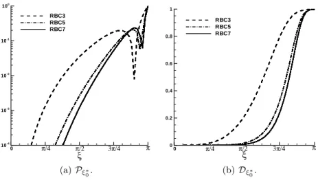
The spectral properties of RBC schemes of different orders, i.e. the dispersion error and damping function for a given Fourier mode have been investigated in [9]. Fig. 1(a) shows the phase errors (in log scale) for RBC schemes of different orders as a function of the reduced wavenumber, for a linear advection problem along a grid direction (1D case). Tab. 1 provides the wave number corresponding to an error of 10−3. RBCq schemes of fifth- and seventh-order accuracy exhibit a cut-off wave number ξcvery close to π/2, the smallest resolvable wave number
being close to 2π/5 according to Nyquist criterion. Similarly, Fig. 1(b) provides the damping functionDξ∗0. As it can be seen in Tabs. 2, RBC5 and RBC7 exhibit
a damping function of less than 10−3 up to cut-off wave numbers of 1.03 and 1.24, respectively, which raises sharply at higher wave numbers. This shows that the intrinsic numerical dissipation of high-order RBCq schemes acts as a selective filter with a sharp cut-off at high frequency: it efficiently damps out grid-to-grid oscillations that can lead to numerical instabilities without affecting the resolved wave numbers. Also note that, coherently with the truncation error analysis, the resolvability limit of RBC schemes is essentially ruled by the dissipation and not by the dispersion error, their leading-order error term being of dissipative nature. The results summarized in Tab. 1 and 2 prove that RBC schemes of order 5 and 7 can accurately resolve a given wavelength by means of less than 7 or 6 mesh cells respectively, whereas RBC3 requires approximately 9 mesh cells to meet the prescribed accuracy requirements on dispersion errors and 16 mesh points for dissipation errors. For comparison, typical second-order schemes used in industrial codes have a resolvability of 20 to 30 points per wavelength.
ξ 10-4 10-3 10-2 10-1 100 RBC3 RBC5 RBC7 π/2 π/4 0 3π/4 π (a)Pξ0∗. ξ 0 0.2 0.4 0.6 0.8 1 RBC3 RBC5 RBC7 π/2 π/4 0 3π/4 π (b)Dξ∗0.
ξc λc/δx RBC3 0.74 8.47 RBC5 1.39 4.53 RBC7 1.54 4.07
Table 1. Resolvability limit due to
disper-sion of RBC schemes.
ξc λc/δx RBC3 0.40 15.56 RBC5 1.03 6.08 RBC7 1.24 5.06
Table 2. Resolvability limit due to
dissi-pation of RBC schemes.
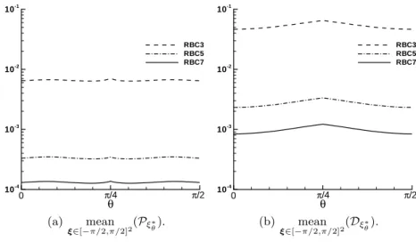
Then, spectral properties of RBCq schemes were also investigated in the case of multidimensional advection. An overview of the phase and damping error for the range of advection directions, θ∈ [0, π/2] is provided in Fig. 2, showing the average value of Pξθ∗ and Dξ∗θ for ξ ∈ [−π/2, π/2]2. Thanks to their genuinely
multi-dimensional formulation, RBC schemes provide an almost constant error level over the whole range of advection direction, with a maximum at θ = π/4 and a minimum at θ = 0 and θ = π/2. Furthermore, error levels decrease quickly with the order of accuracy.
θ 10-4 10-3 10-2 10-1 RBC3 RBC5 RBC7 π/4 π/2 0 (a) mean ξ∈[−π/2,π/2]2(Pξ∗θ). θ 10-4 10-3 10-2 10-1 RBC3 RBC5 RBC7 π/4 π/2 0 (b) mean ξ∈[−π/2,π/2]2(Dξ∗θ).
Fig. 2. Average ofPξ∗θ andDξ∗θ over the interval ξ∈ [−π/2, π/2]2as a function of the advection direction θ.
3
Extension to complex geometries
RBC schemes, developed in a regular Cartesian grid framework by using finite-difference approximation operators, are extended to general curvilnear grids by means of a cell-centred finite volume formulation, such that the problem un-knowns are the point-wise values of the conservative variables at cell centers. A finite volume RBC scheme can be expressed again under the general form (3)
with the dissipation operator (4), provided that the local residuals r are replaced by integrated residuals R over the computational cell (for the main residual) or over a shifted cell (for the mid-point residuals). Details can be found in [10]. For such a straightforward FV extension the nominal order of accuracy is not pre-served on non-uniform curvilinear meshes. Ref. [11] shows, in the framework of non compact schemes, that nominal accuracy can still be preserved if the mesh satisfies suitable regularity conditions. The higher the scheme accuracy, the more stringent grid regularity requirements, so that nominal accuracy is generally lost for cases of practical interest. In order to ensure high-accuracy on curvilinear grids while avoiding expensive finite-element like reconstructions of the solution over une cell, two strategies can be adopted. The first-one consists in developing a high-accurate finite volume discretization making use of weighted discretiza-tion operators to take into account mesh deformadiscretiza-tions while still taking benefit of the structured grid formulation: specifically, this strategy has been used to develop a curvilinear grid extension of the RBC scheme of nominal 3rd-order ac-curacy. The second one consists in maximizing the regions of the computational domain that are discretized with Cartesian grids: this is achieved by developing an overset grid strategy using curvilinear grid blocks close to solid walls, while covering the rest of the domain by means of Cartesian grid blocks. The main features of both strategies are briefly described in the following.
3.1 High-accurate finite volume formulation
We consider a RBC finite volume scheme of the general form:
( ˜R0)j,k,l= ˜dj,k (21)
where ˜R0, called the main residual, is a space-centered approximation of R and
˜
d is a residual-based dissipation term, introduced to ensure numerical stability,
defined in terms of first-order differences of the residual as: ˜ dj,k= 1 2[δ1(Φ1 ˜ R1) + δ2(Φ2R˜2)]j,k (22)
where ˜R1and ˜R2, respectively defined at (j +12, k) and (j, k +12), are also
space-centered approximations of R on a suitably chosen shifted control volume, are called the mid-point residuals, and Φ1, Φ2are the previously defined dissipation
matrices.
In Ref. [10], compact approximations of the main and mid-point residuals were constructed based on weighted approximation operators. With such an approach, it was possible to construct an RBC scheme of third-order accuracy on Cartesian meshes and at of second-order accuracy at least on general deformed meshes. We refer to [10] for details. Such an approach is more accurate than the straightforward finite volume counterpart of RBC schemes, while introducing only a moderate overcost in terms of CPU time and memory requirements. An analysis of the truncation error and spectral properties of this scheme, also discussed in [10] shows that this scheme is slightly more dissipative than its
finite-difference counterpart. Nevertheless, this (small) extra dissipation ensures robusteness on strongly distorted grids and is compensated by the better overall accuracy of the approximation.
3.2 Overset grid strategy
We define an overset mesh in D dimension(s) as a mesh composed of M ordered component grids {Gm}m∈[1,M] of the spatial domain Ω ⊂ RD. The ordinal of
the grid defines its priority in the overset assembly algorithm. An assembly algorithm is used to determine the connectivity (or localization) of points that must exchange information between component grids. Considering a point P ∈
Gm, this step consist in finding whether or not P lies within grid Gm′ and, if so,
to find a base point Q∈ Gm′ corresponding to the centroid of the cell of Gm′ in
which lies point P . A brute force search algorithm being too costly in terms of computational effort, we apply several preconditioning steps, described in [12].
Once grid connectivities have been determined, the next step is to interpolate the solution between overset grids. For this purpose, we use Lagrange interpo-lation formulae based on polynomials of even order N = q + 1, with q the (odd) order of accuracy of the inner-point scheme in use. To achieve such interpola-tions, we use transfinite interpolation where the mesh is not too distorted and we use the iso-parametric mapping method where the transfinite interpolation fails. The iso-parametric mapping was introduced in Ref. [13], extended to high-order in Ref. [14] and used for aeroacoustics simulations for instance in Ref. [15].
We refer to [12] for further details about the connectivity search algorithm and Lagrange interpolation techniques.
4
Implementation details
Finite volume extensions of RBC schemes up to fifth-order accuracy have been implemented in the elsA code developed by ONERA. This code is used for the turbomachinery applications shown in Section 5.3. We refer to the elsA user manual for details about the code [17].
On the other hand, finite volume RBC schemes up to 7th-order accuracy in conjunction with the overset grid strategy have been implemented in a in-house code, named DynHoLab [16]. DynHoLab can handle different governing equations both in two and three dimensions of space. At the present stage of development, the code uses a finite volume methodology on multi-block struc-tured meshes. DynHoLab is coded using a combination of a compiled and type-safe language (FORTRAN) with an interpreted and dynamically typed language (Python [18]). Thanks to this, it benefits from the fast and safe execution of the first one, along with easy and fast development capabilities thanks to the second one. The data-structure chosen for DynHoLab is a CGNS-tree [19] which pro-vides a full hierarchical structure to store the data. The code framework handle parallel computations through an MPI implementation which is based on the intrinsic multi-block architecture of DynHoLab. Thus, it is possible to manage
structured as well as unstructured tessellations of the computational domain. Figure 3 illustrates the weak and strong scalability properties of the code. This is led with the cheapest scheme implemented (among high-order schemes) which correspond to the worst case for a scalability study. The code appears to be scalable up to one thousand cores using blocks of 503 cells. On the other hand,
the code exhibit an efficiency close to 0.9 up to 2048 cores.
101 102 103 N 1 1.2 1.4 1.6 1.8 2 2.2 2.4 2.6 2.8 Ta d im 32x32x32 50x50x50 60x60x60
(a) Weak scalability: Time per iteration per cell as a function of the processing units 101 102 103 N 101 102 103 sp e e d -u p DynHoLab Ideal
(b) Strong scalability: Speed-up as a function of the processing units (log-log)
Fig. 3. Scalability of DynHoLab
In both elsA and DynHOLab codes, the RBC schemes are used in conjunction with nominally second-order accurate approximations of the viscous terms and of the boundary conditions. The last choice is expected to have an impact on the overall convergence order of the simulations and will be improved in the future. For steady problems, the solution is advanced through a time marching pro-cedure. The equations are discretized in time by means of the robust first-order Euler method. To reduce computational costs and preserving code modularity, deferred-correction strategy based the Roe-Harten first-order upwind implicit operator is adopted, which is solved by means of L-U factorization. For un-steady problems, the time derivative is approximated through the second-order accurate backward linear multistep scheme (Gear’s scheme). The resulting non-linear system of equations is then solved through Newton-subiterations. The number of subiterations is such that the residual converges by at least 3 orders of magnitude at each time step.
5
Numerical applications
In the first part of this Section, RBC schemes are applied to selected test cases. The first one is a simple inviscid transonic flow over an NACA0012 airfoil. This test case, proposed in the 1st and 2nd workshop on high-order methods [20, 21], is used for a preliminary validation of the proposed schemes and of the overset
grid strategy. Then, RBC schemes are applied to scale-resolving simulations, to demonstrate the excellent resolvability properties of these schemes. Finally, we demonstrate the robustness and the accuracy of RBC schemes for some chal-lenging transonic turbomachinery configurations.
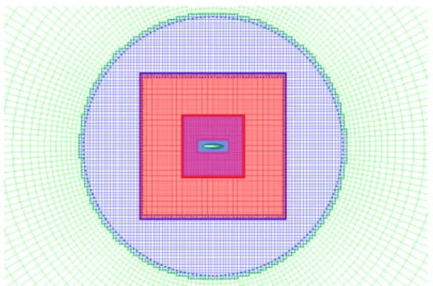
5.1 Preliminary validation: inviscid flow over an NACA0012 airfoil The first test-case is the inviscid two-dimensional flows over a NACA0012 at transonic conditions M = 0.8 and α = 2.250. The simulations are carried out
using an overset grid composed by a combination of Cartesian and curvilinear grids (see Fig. 4). Precisely, the grid results from the superposition of four Carte-sian grids of 200×90, 140×140, 140×140, and 140×140 cells, an O-shaped body grid of 500× 20 cells, and a background polar grid of 200 × 36 cells. A blanking algorithm is used to remove from the computation cells that are overlapped by grids with a higher priority level, so that in practice the solution is computed by using 75647 degrees of freedom. In the following, the overset grid solution is compared to that obtained on a single-block O-shaped grid made of 601× 147 grid points (88347 degrees of freedom)
Figure 5a illustrates the computed isolines of the Mach number using an RBC scheme of 3rd-order accuracy. Shocks are captured in a sharp and almost non-oscillatory way. Present results are found to be in general good agrement with those collected at the first international workshop on High-Order Methods [20], and are superposed to those obtained for a single-block computation. This is confirmed by inspection of the Mach number distribution along the airfoil wall (see Fig. 5b) and of the aerodynamic coefficients, equal to Cl = 0.3519
and Cd = 0.2265× 10⁻¹ respectively. Compared to single block computations,
the overlapping strategy allows a more efficient distribution of the degress of freedom, and thus a better overall accuracy.
X m a c h 0 0.2 0.4 0.6 0.8 1 0 0.2 0.4 0.6 0.8 1 1.2 1.4 overset mesh single bloc (a) (b)
Fig. 5. Transonic flow over a NACA0012: comparison of an overset grid and a
single-block grid solution. a) Mach isolines; b) wall distributions of the Mach number.
5.2 Scale-resolving flow simulations
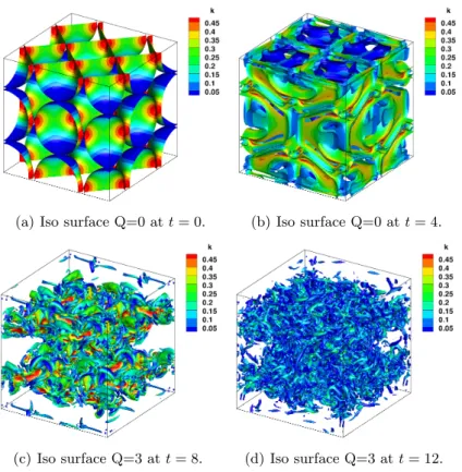
Taylor-Green vortex. The second application, also taken from the 2nd In-ternational Workshop on High-Order CFD Methods [20, 21], is used to study the resolvability properties of high-order schemes in view of subsequent application to fine-scale turbulence simulations. A three-dimensional vortex is set as an ini-tial condition for 3D-computation in a periodic box [0, 2π]3, then it breaks down, giving origin to smaller and smaller structures. Hereafter we carry out a series of Implicit Large Eddy Simulations (ILES) where the main role of the SGS model, i.e. energy drain at small scales, is taken by the numerical dissipation of RBC schemes.
Fig. 6 shows the evolution of an isosurface of the Q criterion at different times. The vortex is initially deformed through vortex stretching and vortex tilting me-chanics, that vortex filaments blow up and the flow transitions to the turbulent regime. Finally, turbulence decays.
The initial conditions of the computation are:
u(x, y, z, 0) = sin(x) cos(y) cos(z)
v(x, y, z, 0) =− cos(x) sin(y) cos(z)
w(x, y, z, 0) = 0
ρ(x, y, z, 0) = 1
p(x, y, z, 0) = p0+
ρ
16(cos(2z) + 2)(cos(2x) + cos(2y))
Where we choose p0 = 100, a Mach number M0 = 0.1, a Reynolds number
Re = 1600 and a Prandlt number P r = 0.71. For these conditions, previously
computed by Brachet [22] using a spectral method, a recent reference DNS ob-tained on a mesh of 5123 cells with a pseudo-spectral code over a quite long
interation time is available [21].
Solutions are computed on a series of structured meshes of 643, 1283, 2563
(a) Iso surface Q=0 at t = 0. (b) Iso surface Q=0 at t = 4.
(c) Iso surface Q=3 at t = 8. (d) Iso surface Q=3 at t = 12.
Fig. 6. Iso surface of the Q criterion colored by k (computed with RBC5 on the 1283
mesh). The figure show phases of the vortex break-up.
CFL number is approximately equal to 5, which is slightly smaller than typical CFL numbers used for industrial LES.
The absence of external forcing implies that the kinetic energy is only decay-ing durdecay-ing the computation. In the followdecay-ing, we look at the time derivative of the kinetic energy integrated on the whole computational domain,−dK/dt, i.e. the kinetic energy dissipation rate, and at the integrated enstrophy Ω. Figure 7a shows mesh convergence for RBC5. For these scheme the solution is already in reasonable agreement with the reference one when using a grid with 643 DOF. Note that, even if the energetically relevant scales are well captured by the sim-ulation, the solution is still far from a converged DNS: this is illustrated by Fig. 7b, which shows the time evolution of the integrated enstrophy for the RBC5 scheme. Enstrophy is more difficult to match than the dissipation rate of the kinetic energy since it requires capturing accurately not only the velocity field but also its gradients [29] up to small flow scales. Note that, for high grid resolu-tions, mesh convergence of RBC5 is slown down by numerical errors introduced by the time integration scheme. This will be improved in the next future.
t -d K /d t 0 4 8 12 16 0 2 4 6 8 10 12 5123Ref 3843 2563 1283 643 323 t E n s tr o p h y 0 4 8 12 16 0 2 4 6 8 10 12 Spectral (5123) energy (3843) enstrophy (3843 ) enstrophy (2563 ) enstrophy (1283 ) enstrophy (643) enstrophy (323)
Fig. 7. Mesh convergence of the time evolution of the total energy (left) and enstrophy
right). RBC5 scheme. time ε 0 5 10 15 0 0.002 0.004 0.006 0.008 0.01 0.012 0.014 5123Ref RBC3 RBC5 RBC7 time ε 0 5 10 15 0 0.002 0.004 0.006 0.008 0.01 0.012 0.014 5123 Ref RBC3 1283 RBC5 643
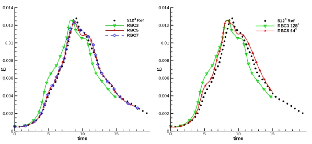
Fig. 8. Time evolution of the total energy for different RBC schemes, 1283grid (left). Comparison of the resolvability properties of RBC3 and RBC5 (left).
Figure 8a compares solutions provided by RBC schemes of different orders on the 1283grid. The relatively small differences between RBC5 and RBC7 are
due to the fact that, for sufficiently high spatial resolution, numerical errors are essentially due to the second-order time discretization scheme in use, which is the same for all computations. On the other hand, RBC5 overperforms RBC3, providing the same or better accuracy on a grid of 643 DOF only (Fig. 8b).
Even if RBC5 is about 3.25 more expensive than RBC3 (mainly due to the higher level of convergence of the residuals required at each time step), it allows a reduction by a factor 16 of the DOF in time and space required to achieve
a given resolution, leadingin turn to a reduction by roughly a factor 4 of the computational effort required to achieve a given accuracy.
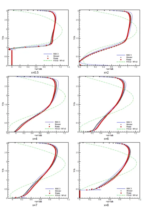
2D periodic hill. A very large implicit large eddy simulation (ILES) of the flow over a periodic 2D-Hill was carried out using the RBC scheme of 3rd-order accuracy. The computations were conducted for an average Mach number of 0.1 and an average Reynolds number of 10595. The flow is driven by a forcing term counteracting the drag force exerted on the channel walls. The forcing term is updated at each time step as a function of the instantaneous space-averaged mass flow. The wall temperature is imposed.
The calculations were carried out on a structured grid made of 64× 32 × 32 cells, corresponding to the coarsest linear grid used for the 2nd workshop on High-Order Methods [21]
The calculations were initialized with a uniform field. The simulation took about 50 convective periods (based on the streamwise length L of the compu-tational domain and the bulk velocity at the throat section Ub, a convective
period being given by T = L/Ub) to reach a statistically steady state. Then,
statistics were collected over 9 additional periods. Calculations were carried out by using a constant time step, taken equal to 10−2T . Fig. 9 shows the averaged
fields of the streamwise velocity < u >, as well as mean streamlines. Figs 10 and 11 display the average streamwise velocity and shear Reynolds stress profiles at different streamwise locations. Present results are compared to the reference LES of Breuer et al. [23], obtained on a grid of about 13 million cells by using a second-order centred finite volume scheme, to the experimental data by Rapp [23] and to results obtained by using a second-order accurate central difference scheme with second-order filtering (denoted FDo2-SFo2). Present results show that RBC scheme provides results in reasonably good agreement with the ref-erence data, at least for first-order statistics, despite the extremely coarse grid in use. The RBC solution represents a dramatic improvement over the solution provided by the standard second-order scheme, which does not even capture the correct trends, since numerical errors introduced by the filter tend to laminarize the flow. This is confimed by the fact that Reynolds stresses for this scheme are virtually null, so that they are not represented on Fig. 11.
5.3 RANS simulations of complex turbomachinery configurations The applications discussed in this section aim at illustrating the capabilities of RBC schemes for the numerical simulation of industrially relevant configura-tions in turbomachinery, with focus on transonic turbomachinery with strong shock waves. The numerical simulations were carried out by using RBC schemes implemented in ONERA’s code elsA.
Rotor37 The NASA Rotor 37 is an isolated transonic axial flow compressor rotor with 36 blades. Extensive experimental data have been collected for this
Fig. 9. ILES of the flow over a periodi 2D Hill. Mean steamwise velocity contours and
mean streamlines
case with the aim of validating the predictive capabilities of numerical simula-tion codes and models ([24, 25]). Numerical studies available in the litterature focus mainly on the assessment of turbulence models for the Reynolds-Averaged Navier–Stokes (RANS) equations and Large Eddy Simulations (LES). RANS simulations often fail to predict the global and local flow properties of NASA Rotor 37, due to the complex physical phenomena taking place in this configu-ration (shocks, shock/boundary layer interactions, sepaconfigu-ration, shock/tip leakage vortex interactions). If the impact of physical models on numerical predictions of the Rotor 37 flow has been extensively studied, the effect of numerical dis-cretizations has been paid much less attention (an exception is represented by [26]), especially for orders of accuracy greater than two, also because of the dif-ficulty of achieving a robust behaviour of higher-order schemes for this kind of challenging configurations.
In the following, we focus on numerical simulations of the Rotor37 configu-ration for operating conditions corresponding to the design rotational speed and to a mass flow rate equal to 98% of the choke conditions. We solve the steady Reynolds-Averaged Navier-Stokes (RANS) equations supplemented by the one-equation Spalart-Allmaras turbulence model. Numerical computations were run using a series of three meshes made up by six structured blocks with conformal joins. The finest grid is clustered enough close to the walls so to be relevant for low-Reynolds computations. The coarsest grid uses values of y+greater than 10. The main properties of these meshes are given in Tab. 3. The medium and coarse grids are obtained through successive agglomerations of neighbouring cells (eight by eight) of the finest one.
Boundary conditions based on local 1D Riemann invariants are used at inlet and outlet boundaries. At the inlet, total pressure and temperature, as well as
Fig. 10. ILES of the flow over a periodi 2D Hill. Mean steamwise velocity profiles
flow direction are imposed. At the outlet, the static pressure distribution is im-posed and iteratively adjusted in order to achieve a prescribed target mass flow. The walls are assumed to be adiabatic. Numerical computations were carried
Fig. 11. ILES of the flow over a periodi 2D Hill. Reynolds shear stress profiles
out with a CFL number equal to 5 for all cases. Computations were stopped once the relative variation in mass flow rate was lower than 0.5%.
Figure 12 provides an overall view of the computed flow field provided by the RBC3 scheme on the finest grid. The flow field is characterised by a bow shock
Table 3. Computational grids.
Grid Cell count Cell layers in the tip clearance y+
Fine 1 480 704 24 2
Medium 185 088 12 5
Coarse 23 136 6 15
upstream of the blade, as well as a passage shock leading to boundary layer separation. A complex shock structure is also present in the tip clearance. Shock sharpness and size of the separation bubble vary according to the scheme in use: the sharpest shock and the greatest separation bubble are provided by RBC3. results are compared with those provided by the classical Jameson’s scheme, the baseline solver in elsA. The latter tends to smear shocks and leads to a smaller separation bubble. Note also that the high-accurate scheme predicts a higher maximum value of the Mach number in the computational field: precisely, maximum values of 1.907, 1.844, and 1.828, are obtained for RBC3, RBC2, and Jameson’s scheme, respectively. RBC3 and RBC2 give quite similar results, the shock at the suction side being captured slightly more sharply by RBC3.
Figure 13 displays the radial distributions of rotor performance at an axial station located 10.67 cm downstream of the blade leading edge. For this station, experimental measurements of the radial distributions of total pressure ratio, total temperature ratio, and adiabatic efficiency are available. Results provided by RBC schemes of 2nd and 3rd order accuracy are in reasonably good agree-ment with the experiagree-ments already on the medium grid, whereas a finer grid is necessary to obtain similar accuracy with Jameson’s scheme. This is better seen in Fig. 14, which compares the radial pressure ratio distributions obtained with the three schemes on the two finer grids.
To complete the discussion, the computational cost of RBC schemes is com-pared to the cost of Jameson’s scheme. The present computations were run on a PC using X5660 Xeon exacore processors with a clock frequency of 2.8Ghz. Computations run with the elsA code were parallelized on two cores using MPI. With this configuration, the computational cost per iteration and per point was of about 0.0125 sec using Jameson’s scheme. The global computational cost is the CPU time required to achieve an almost converged mass flow. All of the schemes achieve the required tolerance level within almost the same number of iterations (about 3000). RBC schemes are more expensive than Jameson’s scheme in terms of operation count: precisely, the computational costs per iter-ation and per point of RBC2 and RBC3 are about 1.8 and 2.2 times greater, respectively. Nevertheless, RBC schemes are clearly more accurate, since they provide almost grid-converged solutions using about 1/8 of the mesh cells re-quired by the baseline scheme. RBC3 is slightly more expensive than RBC2, mainly because of the computation of weighting coefficients, but the extra cost is compensated by a somewhat better accuracy. It is concluded that, for this steady RANS case, using a well-designed, low dissipative scheme has a stronger effect in terms of improved accuracy of the solution than increasing the formal
order of accuracy, so that satisfactory results can be obtained already for a RBC scheme of 2nd-order accuracy. Conclusions are likely to be different unsteady RANS and LES computations. Further research will focus on the application of high-order RBC schemes to scale-resolving unsteady simulations.
X Y
Z
Fig. 12. Overall view of the flow field (98% choke conditions). Mach number
distribu-tion at midplane, and stream ribbons colored by the Mach number. RBC3 scheme.
High-pressure BRITE turbine stage As a final application, the RBCi scheme is used to compute the BRITE HP turbine stage experimentally tested in the compression tube facility CT3 of the Von Karman Institute [27] at high vane exit Mach number (pressure ratio 5.11). This case is computed in order to demonstrate the applicability of the proposed methodology to complex unsteady 3D cases, like a realistic turbine configuration including tip clearance.
The computational grid contains approximately 3 millions of cells and is com-posed by twelve blocks: both the rotor and the stator are discretised by an O-shaped grid around the blades and three H-shaped blocks for inlet, outlet, and inter-blade regions; the tip clearance is also discretized with an O-shaped and three H-shaped grids. Unsteady computations are initialised with steady results obtained by imposing a mixing-plane inter-stage condition. The use of chorochronic periodic boundary conditions [28] allows simulating just one blade per row. The flow is modelled through the RANS equations completed by the Spalart-Allmaras transport-equation model for turbulence. The governing equa-tions are advanced in time via a dual-time stepping technique: the physical time step is approximately 1/100 of the rotation period and about 30 sub-iterations per time step were used to converge the solution in pseudo-time.
RBCi allows sharp capturing of shock waves and von Karman vortices in the blade wakes (see 15, Fig. 17. Fig. 15 shows a snapshot of the 3D vortex
struc-Fig. 13. Radial performance distributions for several schemes and grid resolutions.
Mesh convergence study
Fig. 14. Radial pressure ratio distributions for several schemes and grid resolutions.
tures within the geometry with an isosurface of the Q-criterion colored by the entropy showing the 3D nature of the flow field.
The complex unsteadiness of the flow with rotor/stator interaction is also cap-tured. Fig. 16 provides the Fourier spectra of of the normalized mass flows at stator outlet, rotor inlet and rotor outlet. The main frenquency at the stator outlet corresponds to the adimensional passage frequency of rotor blades with regard to the stator, frotor = 0.016, with its first harmonic confirming that the
rotor/stator interaction is taken into account. Similarly the main frequency ob-served on rotor mass flows at inlet and outlet is the adimensioned frequency of passage of stator blades with regard to the rotor, fstator = 0.011, with its first
harmonics. The high frequency peak of low magnitude at fvort = 0.116 in the
stator spectrum is likely to correspond to the vortex shedding at the trailing edge of the stator blades since it does not match the frequency of an harmonic and its magnitude is too high. This frequency is seen by the rotor at a slightly different frequency probably because of the chorochronic periodicity conditions applied between the rotor and the stator, which filter the signal.
Fig. 17 provides a snapshot of three slices of the configuration located near the hub, at mid span of the blades and near the rotor housing. The slices represent entropy contours along with isobars. Strong shocks are created at the trailing edge of the stator and rotor blades near the hub. Morover the differences be-tween these three slices confirm that this case is highly three-dimensional with a major impact of the tip clearance on the wake of the rotor blades.
Fig. 15. VKI BRITE HP turbine: snapshot of Q criterion isosurface, Q=0.001, colored
Freq M a s s fl o w 0 0.05 0.1 0.15 0 0.2 0.4 0.6 0.8
(a) Stator outlet.
Freq M a s s fl o w 0 0.05 0.1 0.15 0 0.2 0.4 0.6 0.8 (b) Rotor inlet. Freq M a s s fl o w 0 0.05 0.1 0.15 0 0.2 0.4 0.6 0.8 (c) Rotor outlet.
Fig. 16. VKI BRITE HP turbine:: mass flow frenquency spectrum.
(a) Slice near the hub. (b) Slice at mid span of the
blades.
(c) Slice near the rotor
housing.
Fig. 17. VKI BRITE HP turbine: slices of the solution at different spanwise locations;
6
Conclusions
A family of high-order Residual-Based compact schemes has been extended to unsteady flows and complex geometries. Unsteady RBC schemes of highest order (5 and 7) exhibit excellent resolvability properties, since their genuinely multi-dimensional numerical dissipation acts as a sharp cutoff filter close to the grid resolvability limit. In practice, very encouraging results were obtained for a very coarse implicit large eddy simulation of the separated flow over a periodic 2D hill by using an RBC scheme of 3rd-order accuracy. RBC schemes, developed in a finite difference framework, were extended to geometrically complex con-figurations by means of a robust and accurate finite volume formulation and an overset grid strategy. Applications to severe transonic turbomachinery flows prove the robustness of the proposed approach and show that significant gains, both in terms of degrees of freedom and workunits required to achieve a given numerical error level, can be obtained with respect to traditional finite volume schemes in use in industry.
References
1. Lerat, A., Corre, C.: A residual-based compact scheme for the compressible Navier-Stokes equations. Journal of Computational Physics,= 170, 642675 (2001). 2. Lerat, A., Corre, C.: Residual-based compact schemes for multidimensional
hyper-bolic systems of conservation laws. Computers & Fluids 31, 639661 (2002). 3. Deconinck, H., Ricchiuto, M.: Residual Distribution schemes: foundation and
anal-ysis. In: Encyclopedia of Computational Mechanics, John Wiley and Sons, Ltd. (2007).
4. Abgrall, R.: Residual distribution schemes: Current status and future trends. Com-puters & Fluids 35, 641669 (2006).
5. Lerat, A., Corre, C.: Higher order residual-based compact schemes on structured grids. In: 34th Comput. Fluid Dyn. Course, von Karman Institute for Fluid Dy-namics, VKI LS 2006-1, 1111 (2006).
6. Corre, C., Hanss, G., Lerat, A.: A residual-based compact scheme for the unsteady compressible NavierStokes equations. Computers & Fluids 34, 561580 (2005). 7. Corre, C., Falissard, F., Lerat, A.: High-order residual-based compact schemes for
compressible inviscid flows. Computers & Fluids 36, 15671582 (2007).
8. Lerat, A., Grimich, K., Cinnella, P.: On the design of high order residual-based dissipation for unsteady compressible flows. Journal of Computational Physics 235, 3251 (2013).
9. Grimich, K., Cinnella, P., Lerat, A.: Spectral properties of high-order residual-based compact schemes for unsteady compressible flows. Journal of Computational Physics 252, 142-162 (2013).
10. Grimich, K., Michel, B., Cinnella, P., Lerat, A.: An accurate finite-volume for-mulation of a Residual-Based Compact scheme for unsteady compressible flows. Computers & Fluids 92, 93-112 (2014).
11. Rezgui, A., Cinnella, P., Lerat, A.: Third-order finite volume schemes for Euler computations on curvilinear meshes. Computers & Fluids 30, 875901 (2001).
12. Outtier, P.Y., Content, C., Cinnella, P.: High-order residual-based compact schemes for compressible flows on overset grids. 32nd AIAA Applied Aerodynamics Conference, AIAA Aviation and Aeronautics Forum and Exposition 2014. Atlanta, June 2014 (to appear).
13. Benek, J. A., Steger, J. L., Dougherty, F. C., Buning, P. G.: Chimera: A Grid-Embedding Technique. Report AEDC-TR-85-64, Arnold Engineering Development Center, April 1986
14. 28Sherer, S. E. and Scott, J. N., High-order compact finite-difference methods on general overset grids, Journal of Computational Physics, Vol. 210, No. 2, Dec. 2005, pp. 459496.
15. Chicheportiche, J., Gloerfelt, X.: Study of interpolation methods for high-accuracy computations on overlapping grids. Computers & Fluids 68, 112133 (2012). 16. Outtier, P.-Y., Content, C., Cinnella, P., and Michel, B.: The high-order dynamic
computational laboratory for CFD research and applications. 21st AIAA Compu-tational Fluid Dynamics Conference, Fluid Dynamics and Co-located Conferences, American Institute of Aeronautics and Astronautics, June 2013.
17. elsA website, http://elsa.onera.fr/. 18. Python web site, http://www.python.org/. 19. CGNS website, http://cgns.sourceforge.net/.
20. Website of the 1st workshop on High-Order CFD
meth-ods,http://zjwang.com/hiocfd.html
21. Website of the 2nd workshop on High-Order CFD
methods,http : //www.dlr.de/as/desktopdef ault.aspx/tabid− 8170/13999read− 35550/
22. Brachet, M., Meiron, D.I., Orszag, S.A., Nickel, B.G., Morf, R.H., Frisch, U.: Small-scale structure of the Taylor-Green vortex. Journal of Fluid Mechanics 130, 411-452 (1983).
23. Breuer, M., Peller, N., Rapp, C., Manhart, M.: Flow over periodic hills numerical and experimental study over a wide range of Reynolds numbers. Computers and Fluids 38, 433-457 (2009)
24. Suder, K.L.: Experimental Investigation of the Flow Field in a Transonic, an Axial Flow Compressor With Respect to the Development of Blockage and Loss. NASA TM 107310 (1996).
25. Dunham, J., ed.: CFDValidation for Propulsion System Components. AGARD Advisory Report AR-355 (1998).
26. Chima, R.K., M.-S. Liou.: Comparison of the AUSM+ and H-CUSP Schemes for Turbomachinery Applications. AIAA Paper 2003-4120 and NASA TM-2003-212457 (2003).
27. Denos, R., Arts, T., Paniagua, G., Michelassi, V., Martelli, F: Investigation of the unsteady rotor aerodymics in a transonic turbine stage. Journal of Turbomachinery 123 (2001)
28. Gerolymos, G.A., Michon, G., Neubauer, J.: Analysis and application of chorochronic periodicity in turbomachinery rotor/stator interaction computations. Journal of Propulsion Power 18, 11391152 (2002).
29. Donzis, D.A., Yeung, P.K, Sreenivasan, K.R: Dissipation and enstrophy in isotropic turbulence: Resolution effects and scalling in direct numerical simulations. Physics of Fluids, 20:045108 (2008)