HAL Id: hal-00526286
https://hal-mines-paristech.archives-ouvertes.fr/hal-00526286
Submitted on 14 Oct 2010HAL is a multi-disciplinary open access
archive for the deposit and dissemination of sci-entific research documents, whether they are pub-lished or not. The documents may come from teaching and research institutions in France or
L’archive ouverte pluridisciplinaire HAL, est destinée au dépôt et à la diffusion de documents scientifiques de niveau recherche, publiés ou non, émanant des établissements d’enseignement et de recherche français ou étrangers, des laboratoires
Experimental validation of finite element codes for
welding deformations
Harald M. Aarbogh, Makhlouf Hamide, Hallvard G. Fjaer, Asbjørn Mo,
Michel Bellet
To cite this version:
Harald M. Aarbogh, Makhlouf Hamide, Hallvard G. Fjaer, Asbjørn Mo, Michel Bellet. Experimental validation of finite element codes for welding deformations. Journal of Materials Processing Technol-ogy, Elsevier, 2010, 210 (13), pp.Pages 1681-1689. �10.1016/j.jmatprotec.2010.05.014�. �hal-00526286�
Experimental validation of finite element codes for
welding deformations
H. M. Aarbogha,b,∗, M. Hamidec, H. G. Fjærd, A. Moa, M. Belletc
aSINTEF Materials Technology, N-0314 Oslo, Norway.
bUniversity of Oslo, N-0316 Oslo, Norway.
cCEMEF Ecole des Mines de Paris, Sophia Antipolis, France.
dInstitute for Energy Technology, N-2027 Kjeller, Norway.
Abstract
A single pass Metal Inert Gas welding on an austenitic steel plate has been pre-sented for the purpose of providing controlled experimental data against which numerical codes quantifying welding stresses can be validated. It includes a mov-ing heat source with material deposit, and completes thus existmov-ing validation data. The experiment has been addressed by a numerical code, WeldSimS, reproduc-ing qualitatively the distortion durreproduc-ing weldreproduc-ing quite well. Quantitative differences between the numerical and experimental results, however, indicate the need for more accurate modelling tools than those presently available, which are all based on commonly accepted modelling principles and input data.
Keywords: deformations, constitutive equations, steels, welding, finite element modelling.
PACS: 46.80.+j, 46.15.-x
1. Introduction
During welding of e.g. steel, the heat source leads to rapid heating and melt-ing of the material and the formation of a weld pool that subsequently cools and solidifies. Welding stresses arise due to the inhomogeneous cooling, and in steel these stresses are caused by the effects of non-uniformly distributed cooling con-tractions and, in ferritic steels, solid state phase transformations. Modelling of
∗Corresponding author
Email address: [email protected] (H. M. Aarbogh)
*Manuscript
the welding stresses and associated deformations requires, therefore, a numerical code able to predict both the thermometallurgical and the mechanical develop-ment during the process. Ideally, a numerical code should account for a series of complex phenomena such as the material deposition, weld arc heat input, melt-ing and solidification, solid-state phase transformations, work hardenmelt-ing, strain rate sensitivity, and the flow stress dependency on the specific mixture of phases appearing at the different temperatures. Welding in general includes several me-chanical phenomena such as transverse, longitudinal, and angular shrinkage, as well as bending distortion (Pilipenko, 2001, chap. 2.2).
However, due to this complexity, as well as the need for minimising the com-putation time, simplified models are often applied (Taljat et al., 1998; Ferro et al., 2006; Brown et al., 2006; Dean and Hidekazu, 2006). This means that the codes should be carefully validated against controlled experiments before being used to predict welding stresses in real industrial situations. Such validation experiments have been carried out in the present study. The study also addresses the presented validation experiment numerically, investigating the validity of the numerical code WeldSimS (Fjær et al., 2006) implemented in FORTRAN90 by the Institute for Energy Technology.
Validation cases have previously been published e.g. by Volden (1998) pre-senting a Satoh (1972b,a) experiment, Taljat et al. (1998) who presented welding of a disc, Roux and Billardon (2006) who presented a ”multipass” welding of a disc, and Vincent et al. (1999, 2005), Bergheau et al. (2004), and Depradeux and Jullien (2004a,b) at INSA-Lyon who also presented a Satoh experiment and a disc experiment in addition to a single pass Tungsten Inert Gas (TIG) welding. These validation cases include one, two and three dimensional cases represented by the Satoh test, a disc case, and a plate experiment, respectively. They do however not include material deposit.
The experiment of the present study is a single pass Metal Inert Gas (MIG)
welding on an austenitic steel plate, carried out at the CEMEF1 research centre.
By involving material deposit and a moving heat source, our experiment comple-ments the validation cases referred to above. The objectives of the present paper is firstly to present a validation experiment that completes existing work. Secondly, the present study addresses the lack of accuracy in commonly used modelling equations used in welding simulations.
Section 2 of the paper presents the welding case and the experimental details
along with the experimental results. The numerical code including the modelling equations and implementation is summarized in Section 3. The modelling results are presented and compared to the experimental results in Section 4.
2. The welding case
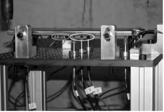
Figure 1 shows the experimental setup including the torch and the sample positioned as when ready to be welded. The thick plate used in the experiment is
Figure 1: The experimental setup including the torch (at the top left) and the sample positioned ready to be welded. The thermocouples and the LVDT (Linear Variable Differential Transformer) sensors can be seen inside the grey and white ellipses, respectively.
furthermore shown in Figure 2. It is 136 mm wide, 10.5 mm thick, and 250 mm long in the welding direction. The geometry was chosen small enough to preform 3D modelling with limited calculation time, but still large enough in the welding direction to obtain a thermal quasi-stationary situation. The weld line is marked in Figure 2 with dashed line, and the torch begins and ends 10 mm from the edges. To measure welding deformations the specimen rests unrestricted on three pins A, B, and C marked with shaded circles in Figure 2.
A one-time-step simulation, computing the stresses without any welding, has been carried out under the assumption that the maximum stress associated with bending moments induced by the supports is of the order 0.5 MPa (0.1% of the yield stress). The resulting peak xx stress is then about 0.2 MPa. The bending of the plate due to gravity was here estimated to be approximately 1µm, which is much less than the welding induced distortions. The authors would therefore
expect the deformation of the plate to vary much less than 1% in cases involving different numbers of support points.
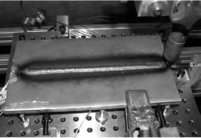
No other clamping or cooling is imposed except the welding electrode holder, which is attached as shown in Figure 3. The plate is thus situated in open air during the whole welding process and subsequent cooling. Three other pins, indicated
(a)
(b)
Figure 2: (a) Sample geometry and the location of the various log points. All dimensions are in mm. (b) Depth of the pre-drilled holes where the thermocouples are attached, along with the dimensions of the plate and the pins where the plate rests, marked with shaded triangles and named A and B in correspondence with the pins marked with shaded discs in Figure 2(a).
by D, E, and F in Figure 2 are used to align the sample to the torch trajectory before welding. Thermal evolution is monitored at twelve different positions (T1 to T12), with depth shown in Figure 2(b). Finally, the displacements are logged at six different points marked with black dots and named C1 to C6, in Figure 2.
The material is ANSI 316LN (Z2CND17-13 in standard Afnor2) widely used
in chemical, oil, and nuclear industry for its resistance to corrosion; see Table 1 for the chemical composition. 316LN is an austenitic steel type and thus do not
Figure 3: View of the welding bench with focus on the support pins and LVDT sensors. Also shown, the welding electrode clamped to the plate.
undergo any phase transformations.
Table 1: Chemical composition (wt %) of 316LN (Hamide, 2008)
C Mn S Ni Cr Mo N Cu
0.02 1.2 <0.001 13.5 17.7 2.6 0.17 0.1
2.1. The experiment
The used power source is a Fronius Transpuls Synergic 4000 shown in Fig-ure 4 along with the test bench, the sample stand, and the movable arm at which the torch is mounted. During the experiment, the voltage, the filler material speed, the shield gas, and the torch speed are controlled, and the resulting current is mea-sured. The welding procedure is automatically controlled by means of a Lab-VIEW software and the displacement sensors are connected to a National Instru-ment SCXI-1540 LVDT Input Module with a sampling frequency of 25Hz. Three parallels, named Test 1, Test 2, and Test 3, were carried out in order to verify the reproducibility.
The temperature evolution is measured inside the plate by forcing 1 mm MgO insulated thermocouples (type K) with steel cap into pre-drilled holes, as indi-cated in Figure 2(b), and glued to the plate with metallic tape. This technique
Figure 4: Overview of the welding bench.
introduces an uncertainty due to the relatively high response time.3 As indicated
in Figure 2(b), the thermocouples are placed to minimize the influence of the ad-jacent thermocouple. The holes were pre-drilled with help of a simple ruler which leads to an uncertainty of 0.5 mm in both x and y direction. The depth of the holes (z-direction) is also believed to have an uncertainty of 0.5 mm, but due to the shape of the drilling tool it might be larger and will be further discussed below. To detect the vertical displacements, six Sensorex SX8 MM05 (see Table 2) LVDT sensors were positioned as indicated in Figure 2 and shown in Figure 3. The Fusion zone (FZ) and the heat effected zone (HAZ) were revealed by
consid-Table 2: Sensorex SX8 MM05 LVDT (Sensorex, 2010)
EM ± 0.5 ± 5 mm Lin. < 0.25 % PE Alim./Sortie AC/AC ToC -10oC to +65oC Dim. Ø8 mm Note IP 65
3Actually, 125 µm type K (Chromel-Alumel) thermocouples were firstly spot-welded to the
plate; however significant disturbances in the measurements during the preliminary test forced us to use the described technique.
ering a cross section orthogonal to the welding direction at S1 and S2 indicated in Figure 2(a). The cross section was polished according to Struers online guide.
Figure 5: Measured welding parameters.
The filler material was a 1.2 mm 316LNSI with a feed speed of 12 m min−1,
the welding voltage was 29 V, and the welding speed was 10 mm s−1. The total
welding length was 230 mm, and welding ended at 23 s. M12 (or Arcal 12) argon
Figure 6: Instrumented test samples align on the bench after the welding.
(Ar) with 1-5 % CO2was used as shield gas and the intensity was controlled
the transitional stages (beginning and end of welding) as shown in Figure 5, while Figure 6 shows the plate after welding. For a more detailed description of the experiment please consult Hamide, 2008.
2.2. Experimental results
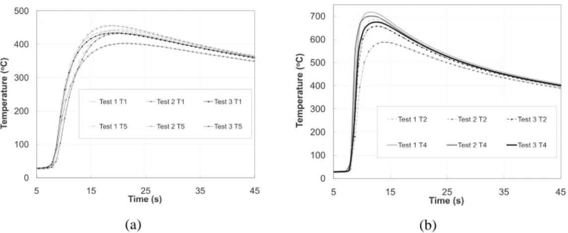
A cross section of the fusion zone with its typical shape is shown in Figure 7, including the holes for attaching thermocouples. Figure 8 reveals some scattering
Figure 7: A cross section of the fusion zone at S1 (see Figure 2) from Test 3. The pre-drilled holes for T1 and T5 are clearly visible at the right and left, respectively.
of the experimental temperatures. However, it also shows that the symmetry in the measurement positions T1 and T5 as well as T2 and T4 is reflected for Tests 1 and 3. In Figure 9, which shows the displacement results, Test 3 reveals a better
symmetry than Test 24. On this basis, we have in Section 4 chosen to compare our
modelling results with Test 3. In the following, all referred experimental results are those obtained in Test 3.
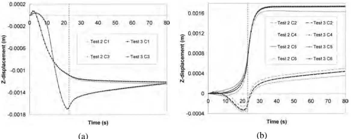
The displacement curve for sensor C3 (Test 3) in Figure 9 reveals some of the involved phenomena. The deflections start with a small positive value due to the influence from the initial heating and following expansion of the top side of the plate. After about 5 s the plate starts to deflect in negative direction due to angular distortion because of inhomogeneous heating and cooling through out the thick-ness of the plate i.e. there is a temperature gradient in z-direction. From 11.5 s, when the source passes C3, the deflection increases and reaches the peak value
500 400 ( oC) 300 ra tu re 200 e mpe
r Test 1 T1 Test 2 T1 Test 3 T1
100
T
e Test 1 T5 Test 2 T5 Test 3 T5
0 5 15 25 35 45 Time (s) Time (s) (a) 700 600 700 500 ( oC) 400 ra tu re 300 e mpe r
Test 1 T2 Test 2 T2 Test 3 T2
200
T
e Test 1 T2 Test 2 T2 Test 3 T2
Test 1 T4 Test 2 T4 Test 3 T4
100
est est est 3
0
5 15 25 35 45
Time (s) Time (s)
(b)
Figure 8: Experimental temperature development from Test 1, 2, and 3: (a) Thermocouples 1(T1) and 5(T5) (b) Thermocouples 2(T2) and 4(T4) (see Figure 2 for positioning).
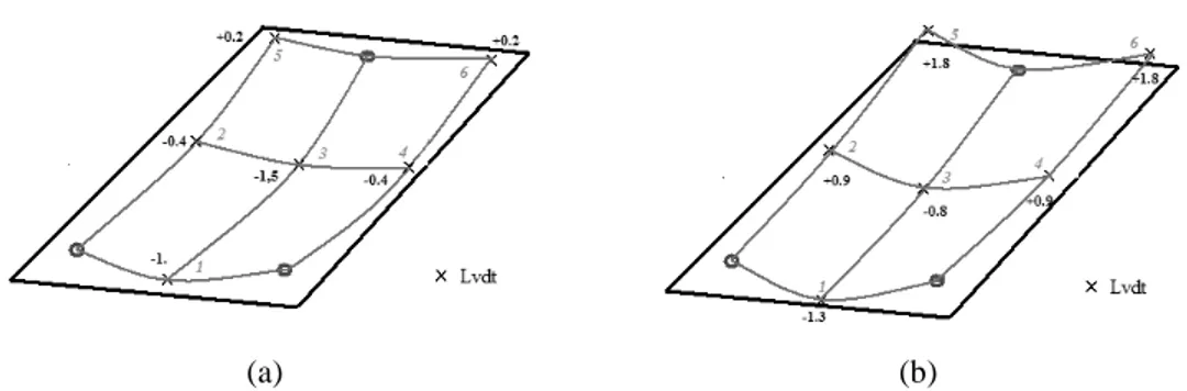
of about 1.8 mm at 22 s. After 23 s (end of welding), the plate starts to cool, and the longitudinal distortion arises forcing the plate to deform in x-direction. This results in a gradually decreasing vertical deflection shaping a noticeable dip in the curve from about 19 s to 23 s. Due to the support pin C, just below the weld path, this decrease of vertical deflection starts somewhat before the welding ends. Figure 10 shows the displacement results up to 500 s, revealing the de-velopment during the whole cooling process. Figure 11 illustrates the distortion (exaggerated) of the plate, after 23 s and 500 s, and shows bending around both the longitudinal (welding direction) and the transverse axis.
3. Modelling
3.1. Governing equations
Neglecting mechanical dissipation and assuming thermal equilibrium at the microscopic scale, the transient heat transfer is governed by (Haug and Langtan-gen, 1997):
ρ cpT + ρ ˙g˙ liq∆H = ∇ · (λ∇T ) (1)
where ρ, cp, λ, T , ∆H, and gliq denote the density, specific heat capacity,
ther-mal conductivity, temperature, latent heat of fusion, and the liquid fraction, re-spectively. Thermal boundary conditions (Mortensen, 1999; Carslaw and Jaeger, 1959, chap. 1.9) include both convection from Fourier’s law and radiation from
(a) (b)
Figure 9: The experimental displacement (Test 2 and 3) for the LVDT sensors C1 and C3 are shown in (a) and C2, C4, C5 and C6 are shown in (b). The vertical dashed lines indicates the end of welding. Please note that the results from Test 3 are symmetric. This is shown in (b) by the overlapping curves of C2 and C4, and C5 and C6, respectively. Notice also that C5 from Test 2 overlaps with C5 and C6 from Test 3. The results from C1 and C3 in (a) are overlapping between Test 2 and Test 3.
Figure 10: The final experimental displacement for the LVDT sensors C1, C2, C3, and C5 from Test 3. The vertical dashed lines indicates the end of welding. Please note that the results from Test 3 are symmetric. This is shown by the overlapping curves of C2 and C4, and C5 and C6, respectively.
Stefan-Boltzmann law; the equations is:
−λ∂T
∂n = h(T − Tair) + ǫω(T
4
(a) (b)
Figure 11: Schematic representation of the distortions at; (a) the end of welding, (23 s) and (b) the end of cooling (500 s). The circles represent the fixed pins A, B, and C shown in Figure 2.
where h, ǫ, ω, and Tair denote the heat transfer coefficient, thermal emissivity,
Stefan-Boltzmann constant, and ambient air temperature, respectively.
Non-uniform thermal contraction due to density variation with temperature is the driving force for the evolution of stresses and deformations. A quasi-static balance is assumed, and the mechanical equilibrium is governed by the Cauchy’s equation (Malvern, 1969):
∇ · σ + ρg = 0 (3)
where σ is the stress tensor, ρ is the density, and g is the body force per unit mass. The strains are assumed to be small so that the total strain ε can be decomposed (Mase, 1969) into thermal (εth), elastic (εe), and viscoplastic (εp) contributions:
ε= εe+ εth+ εp. (4)
The elastic strain is defined by the temperature dependent Hooke’s law, and the volumetric thermal strain is related to temperature by (Mase, 1969):
εth = Z T
Tre f
α(T)dT (5)
where α(T) is the temperature dependent expansion coefficient, Tref is the
refer-ence temperature for zero thermal strain. Below solidus, the material is considered as elastic-viscoplastic (Fjær and Mo, 1990), using a von Mises yield criterion, and under the assumption of isotropic hardening, the effective viscoplastic strain, ¯εp,
and strain rate, ¯˙εp, are related to the effective stress, ¯σ, by:
¯
σ = σY+ k ¯εpn¯˙ε
m
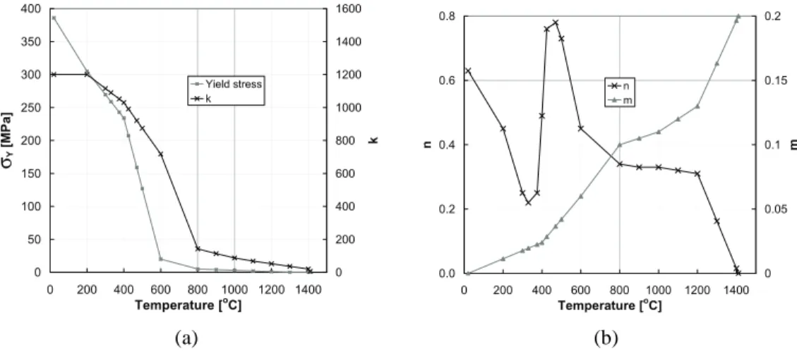
The plastic threshold, σY, the consistency, k, the hardening coefficient, n, and the
strain-rate sensitivity coefficient, m, are temperature dependent functions given in Figures 12 along with the references they were taken from.
0 50 100 150 200 250 300 350 400 0 200 400 600 800 1000 1200 1400 Temperature [oC] σY [ M P a ] 0 200 400 600 800 1000 1200 1400 1600 k Yield stress k (a) 0.0 0.2 0.4 0.6 0.8 0 200 400 600 800 1000 1200 1400 Temperature [oC] n 0 0.05 0.1 0.15 0.2 m n m (b)
Figure 12: The temperature dependent elastic-viscoplastic parameters used in equation (6). All data are taken from Transvalor (2007) and Hamide (2008).
3.2. Model implementation in the numerical codes
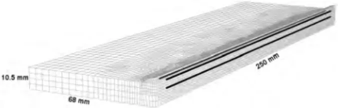
Only half of the plate is included in the numerical model due to symmetry, and Figure 13 shows the dimensions and finite element mesh. As seen in Fig-ure 13 the welding fillet is pre-meshed, but initially these elements are not active (zero density). Only the elements fed enough heat to liquidize are activated and gain density. A graded mesh with high spatial resolution in the fusion zone and the HAZ is required to obtain the necessary numerical resolution. Such refined meshes, using simple 8-noded hexahedral finite elements, have been obtained in a cost-effective way by means of adaptive remeshing (see Table 3 for details). The resulting element size in all cases is of about 1 mm at the weld line. While a
Table 3: Number of elements and nodes.
initial final
nodes 2 140 49 787
Figure 13: Modelled geometry with the three weld lines indicated by the bold black lines. Please note that three heat sources were required for modelling of the experimental single pass welding. In all the cases the fusion plane is treated as a symmetry plane. The figures show the grid density after the simulation is finished.
full integration is used in the thermal problem, a one point (reduced) integration scheme with hourglass control (Belytschko et al., 1984; Liu et al., 1985) is ap-plied for the solution of the mechanical problem. Gradients in thermal strain are here transformed into hourglass strain components on the element level. A robust and simple initial stiffness method as described in Fjær and Mo (1990) is used for quantifying the plastic strains. Appropriate initial guesses and an acceleration scheme improving values for the plastic strain increments ensure a reasonable convergence. To capture the buckling phenomena shown in Figure 11, an updated Lagrangian technique (Belytschko et al., 2000) was used to solve the strain with respect to the current configuration.
3.3. Boundary conditions
The model account approximately for convective heat transfer in the weld pool by enlarging the thermal conductivity by a factor 5 when the temperature is above the liquidus temperature. The chosen factor made the best fit with the fusion zone to the experiment. The temperature dependent material data used for the ANSI 316LN steel are obtained from the database of software package Transvalor Forge (Transvalor, 2007) and shown in Figure 14.
The dimension of the coherent mushy zone is in general less than the element size, and the “stress” viscous effect in the liquid phase is negligible. Furthermore, complete recovery of the hardening in the liquid phase is assumed. The tempera-ture above which relaxation takes place is set equal to the liquidus temperatempera-ture of the chosen material.
The moving heat source (Goldak et al., 1986; Carslaw and Jaeger, 1959, chap. 10.7) is modelled, as a result of a thermal analysis fitting the shape of the fusion zone to the experiment (by varying the heat source’s geometrical parameters),
by two volume heat sources based on double ellipsoidal power density distribu-tions (Goldak and Akhlaghi, 2005, chap. 2.2.2) in addition to one circular surface source with constant heat flux, qs(Goldak et al., 1984):
qs(x, y, t) = 3Q
πr2e
−3[(x−v·t)2]/r2e−3y2/r2, (7)
where Q, v, t, and r denote the total power, welding speed and time, and radius used for the surface source, respectively. Each of the volumetric sources, qv1 and qv2 consists of the ellipsoidals qvi f and qvir (Goldak et al., 1984):
qvi f(x, y, z, t) = 6√3 ffQ abcfπ √ πe −3[(x−v·t)2]/c2 fe−3y2/a2e−3z2/b2, (8) qvir(x, y, z, t) = 6√3 frQ abcrπ √ πe −3[(x−v·t)2]/c2re−3y2/a2e−3z2/b2, (9)
where i is 1 or 2, representing the two volumetric heat sources. ff and fr denote the heat fraction to the front and rear ellipsoidal, fulfilling the relation ff+ fr= 2. Figure 15 illustrates a volume Gaussian double ellipsoidal heat source with all the parameters, and Table 4 lists their used values in addition to the used heat fraction, ff. The first volume source acts on the upper face of the plate, while the second is located inside the plate at z = 6.6 mm. The radius of the circular surface source is 3.5 mm and it is located 3.5 mm from the welding line in the y-direction. The three associated thermal fields overlap (Bonollo et al., 1993) and, represent the single experimental source with the total power (U = 29 V and I = 360 A) sub-divided into 45 % for the first volume source, 15 % for the second, and 40 % for the surface source. These values were obtained by trial and error comparing the
Table 4: Volume Gaussian double ellipsoidal source parameters (see Figure 15).
source a (mm) b (mm) cf (mm) cr(mm) ff (-)
1st 8.5 1.9 8.5 17.0 0.6
2nd 1.3 1.5 1.3 2.6 0.6
calculated shape of the fusion zone to the experimental shape shown in Figure 7. The convective surface heat transfer coefficient in Equation (2) was set to
5 W m−2K−1 (Depradeux and Jullien, 2004a), with a reference temperature (T
of 27oC, while the emissivity was determined by inverse simulation. Due to the
previously mentioned experimental problems in the measured temperature, only the cooling part was applicable for estimation of the involved parameters. The experimental results of T1 in Test 3 from time t=30 s to t=200 s were used in an inverse simulation with the emissivity coefficient and the arc efficiency as vari-ables. From this, an arc efficiency of 0.73 and an emissivity of 0.2 were obtained. To model the three supporting pins on which the plate rests (see Figure 2), spring forces are applied both in normal and transverse directions on small areas representing the experimental pins. These areas were made as small as possible, still obtaining a convergent solution.
4. Modelling results and comparison to the experiment
The temperature development obtained by WeldSimS and the experimental results from Test 3 are shown in Figure 16. The figure shows that the heating rate, heating time, and cooling rate obtained by the numerical codes coincide with the experimental results. However, it is clear that the models overshoot the ex-perimentally measured peak temperature. We believe one of the reasons for this discrepancy is the fact that the temperature was not measured at the very tip of the applied 1 mm insulated thermocouples, and that the contact with the steel sample was not optimal. Also the response time, as mentioned before, might have rep-resented a problem, and the suspension of the thermocouples inside pre-drilled holes might not have been sufficient, as there could have been a small pocket of air above the thermocouples due to the shape of the drilling tools. The parameter study summarized in Figure 17, investigating the influence on the measured tem-perature by varying the z-position of the thermocouples, supports our suspicion that the actual measuring point was not at the expected depth. This study shows that the observed discrepancy corresponds to a misalignment in the z direction of the thermocouple of 2 mm. Also uncertainty in the x- and y-direction contributes to the error. This kind of problems are also reported elsewhere; see e.g. Fig-ure 6.13 in Horn (2003) for a comparison between a welded and a spring-loaded thermocouple. Because of these problems and the fact that there were no thermal measurements in the weld pool, the inversely simulated heat input based on the cooling part of the experiment might be inaccurately estimated.
Since the experimental fusion zone is used to determine the numerical heat source’s geometrical parameters this zone is fairly accurately reproduced by the model, as seen in Figure 18. Note that although the computed fusion line is cali-brated to match the experimental one, the volumetric type heat source is not
con-sidered to represent the actual heat distribution to a very high degree of precision. Figures 19 and 20 display measured and modelled displacements in Test 3. The modelling results are in qualitative agreement with the measurements, although representing a noticeably smaller deflection. In addition to the uncertainties as-sociated with the temperature modelling, the discrepancy could be due to inac-curate constitutive equations and material data; e.g. a too simplistic treatment of hardening and strain relaxation, uncertainties related to the mechanical boundary conditions, as well as the volumetric heat sources. Currently the volumetric heat sources act upon every element inside their geometrical parameters, applying heat to solid elements possibly not in contact with the weld pool. Limiting the vol-umetric heat to liquidized elements and solid elements in contact with the weld pool, could give a larger temperature gradient trough the thickness of the plate, hence larger deformations and a possible reduction of the numerical peak temper-ature shown in Figure 16. We believe that the quantitative differences between the numerical and experimental results indicate the need for more accurate numeri-cal models. This need does not apply only to WeldSimS, but also to most other similar codes, which all are based more or less on the same commonly accepted modelling principles and input data.
5. Conclusions
A single pass Metal Inert Gas welding on an austenitic steel plate, which includes material deposit and a moving heat source, has been presented for the purpose of providing controlled experimental data against which numerical codes quantifying welding stresses can be validated. Some experimental problems, espe-cially the need for more accurate temperature measurements, have been discussed. Improved temperature measurements could in future experiments be addressed by use of thermocouples without steel cap and/or improved attaching techniques, in addition to measurements directly in the weld pool. The present experiment has been addressed by a numerical code, WeldSimS, reproducing qualitatively the dis-tortion during welding quite well. Quantitative differences between the numerical and experimental results, however, indicate the need for more accurate modelling tools, and material data than those presently available, which are all based on commonly accepted modelling principles and input data.
Acknowledgments
The authors wish to express their thanks to Professor Mohammed M’Hamdi, SINTEF and Faculty of Engineering Science and Technology, Norwegian
Uni-versity of Science and Technology, Norway for contribution of relevant input and suggestions. The funding from the research Council of Norway through the ”STORFORSK” Project No. 167397/V30 is greatly acknowledged.
References
Belytschko, T., Liu, W. K., Moran, B., 2000. Nonlinear finite elements for con-tinua and structures. Chichester : Wiley.
Belytschko, T., Ong, J. S. J., Liu, W. K., Kennedy, J. M., 1984. Hourglass control in linear and nonlinear problems. Computer Methods in Applied Mechanics and Engineering 43, 251–276.
Bergheau, J., Vincent, Y., Leblond, J., Jullien, J., 2004. Viscoplastic behavior of steels during welding. Science and Technology of Welding and Joining 9 (4), 323–330.
Bonollo, F., Tiziani, A., Zambon, A., 1993. Model for CO2laser welding of
stain-less steel, titanium, and nickel: parametric study. Materials Science and Tech-nology 9, 1137–1144.
Brown, T., Dauda, T., Truman, C., Smith, D., Memhard, D., Pfeiffer, W., 2006. Prediction and measurements of residual stress in repair welds in plates. Inter-national Journal of Pressure Veddels and Piping 83, 809–818.
Carslaw, H. S., Jaeger, J. C., 1959. Conduction of heat in solids, second edition. Oxford University Press.
Dean, D., Hidekazu, M., 2006. Prediction of welding residual stress in multi-pass butt-welded modified 9Cr-1Mo steel pipe considering phase transformation ef-fects. Computational Materials Science 37, 209–219.
Depradeux, L., Jullien, J.-F., 2004a. 2d and 3d numerical simulation of tig welding of a 316l steel sheet. Numerical Simulation of Welding 13, 269–288.
Depradeux, L., Jullien, J.-F., 2004b. Experimental and numerical simulation of thermomechanical phenomena during a tig welding process. Journal De Physique IV 120, 697–704.
Ferro, P., Porzner, H., Tiziani, A., Bonollo, F., 2006. The influence of phase trans-formations on residual stress induced by the welding process - 3D and 2D nu-merical models. Modelling and Simulation in Materials Science and Engineer-ing 14, 117–136.
Fjær, H., Mo, A., 1990. Alspen - a mathematical model for thermal stresses in di-rect chill casting of aluminium billets. Metallurgical and Materials Transactions B 21, 1049–1061.
Fjær, H. G., Liu, J., M’Hamdi, M., Lindholm, D., 25th September 2006. On the use of residual stress from welding simulations in failure assessment analyses for steel structures. In: H. Cerjak, H.K.D.H. Bhadeshia, E. K. (Ed.), Mathemat-ical Modelling of Weld Phenomena 8. Verlag der Technischen Universitt Graz, pp. 965–979.
Goldak, J., Akhlaghi, M., 2005. Computational welding mechanics. Springer. Goldak, J., Bibby, M., Moore, J., House, R., Patel, B., 1986. Computer Modeling
of Heat Flow in Welds. Metallurgical Transactions B 17, 587–600.
Goldak, J., Chakravarti, A., Bibby, M., 1984. A new finite element model for welding heat sources. Metallurgical Transactions B 15, 299–303.
Hamide, M., 2008. Modlisation numrique du soudage l’arc des aciers (Numerical modelling of steel arc welding). Ph.D. dissertation, Mines ParisTech.
Haug, E., Langtangen, H., 1997. The basic equations in eulerian continuum me-chanics. In: Dæhlen, M., Tveito, A. (Eds.), Numerical Methods and Software Tools in Industrial Mathematics. Birkhauser, Ch. 6, pp. 121–156.
Horn, C. H. L. T., 2003. These. PhD dissertation, Technische Universiteit Delft. Liu, W. K., Ong, J. S. J., Uras, R. A., 1985. Finite element stabilization matrices
– a unification approach. Computer Methods in Applied Mechanics and Engi-neering 53, 13–64.
Malvern, L. E., 1969. Introduction to the Mechanics of a Continuous Medium. Prentice-Hall, Inc.
Mase, G. E., 1969. Theory and Problems of Continuum Mechanics. Schaum’s outline series.
Mortensen, D., 1999. A mathematical model of the heat and fluid flows in direct-chill casting of aluminum sheet ingots and billets. Metallurgical and Materials Transactions B 30, 119–133.
Pilipenko, A., 2001. Computer simulation of residual stress and distortion on thick plates in multielectrode submerged arc welding. Ph.D. dissertation, Norwegian University of Science and Technology.
Roux, G.-M., Billardon, R., 25th September 2006. Identification of thermal boundary conditions and thermo-metallurgical behaviour of x10crmovnb9-1 steel during simple tig welding tests. In: H. Cerjak, H.K.D.H. Bhadeshia, E. K. (Ed.), Mathematical Modelling of Weld Phenomena 8. Verlag der Technischen Universitt Graz, pp. 329–340.
Satoh, K., 1972a. Thermal stresses developed in high-strength steels subjected to thermal cycles simulating weld-affected zone. Transaction of the Japan Welding Society 3, 135–142.
Satoh, K., 1972b. Transient thermal stress of weld heat affected zone by both-ends-fixed bar analogy. Transaction of the Japan Welding Society 3, 125–134.
Sensorex, 2010.www.sensorex.fr.
Taljat, B., Radhakrishnan, B., Zacharia, T., 1998. Numerical analysis of gta weld-ing process with emphasis on post-solidification phase transformation effects on residual stresses. Materials Science and Engineering A 246, 45–54.
Transvalor, 2007. Forge database.www.transvalor.com/forge gb.php.
Vincent, Y., Jullien, J.-F., Cavallo, N., Taleb, L., Cano, V., Taheri, S., Gilles, P., 1999. On the validation of the models related to the prevision of the haz behaviour. ASME Pressure Vessels and Piping Division 393, 193–200.
Vincent, Y., Jullien, J.-F., Gilles, P., 2005. Thermo-mechanical consequences of phase transformations in the heat-affected zone using a cyclic uniaxial test. In-ternational Journal of Solids and Structures 42, 4077–4098.
Volden, L., 1998. Residual stress in steel weldments. PhD Thesis, Norwegian University of Science and Technology.
6800 7000 7200 7400 7600 7800 8000 0 200 400 600 800 1000 1200 1400 Temperature [oC] ρ [kg m-3] 400 500 600 700 800 900 1000 Cp [J kg -1 K -1] Density
Specific heat capasity
(a) 10 15 20 25 30 35 0 200 400 600 800 1000 1200 1400 Temperature [oC] λ [ W m -1K -1] 0 0.2 0.4 0.6 0.8 1 ν [ -] Heat conductivity Poison's ratio (b) 0 50 100 150 200 0 200 400 600 800 1000 1200 1400 Temperature [oC] E [GPa ] 1.5E-05 2.0E-05 2.5E-05 3.0E-05 3.5E-05 4.0E-05 4.5E-05 α [ oC -1] Young's modulus Thermal expantion (c) 0 0.1 0.2 0.3 0.4 0.5 0.6 0.7 0.8 0.9 1 0 200 400 600 800 1000 1200 1400 Temperature [oC] L iq u id fracti o n [-] Liquid fraction (d)
Figure 14: The temperature dependent material data for the steel type 316LN used. The latent heat of fusion in Equation (1) was set equal to 201897 J kg−1All data are taken from Transvalor (2007)
Figure 15: Illustration of a volume Gaussian double ellipsoidal source, indicating the parameters a, b, cf, and cr. 0 100 200 300 400 500 600 700 800 900 6 26 46 66 86 106 Time (s) Te m pe ra tur e ( o C) WeldSimS Tc1 WeldSimS Tc2 Experimental Tc1 Experimental Tc2
Figure 17: Effect of varying the z-position of the thermocouple T2. Changing the numerical measuring position from 7 mm to about 5 mm indicates that a mis-position of about 2 mm would lead to the observed discrepancy between the experimental and numerical results in Figure 16.
Figure 18: Comparison of the fusion zone shape obtained between: numerical and an experimental cross section. The maximum temperature used on the numerical picture is set to 1420oC, making
-0.0018 -0.0016 -0.0014 -0.0012 -0.001 -0.0008 -0.0006 -0.0004 -0.0002 0 0.0002 0 20 40 60 80 100 120 140 Time (s) Z-displacement (m) Exp. C1 Exp. C3 WeldSimS C1 WeldSimS C3
Figure 19: The comparison of LVDT sensors C1 and C3 results with the experimental displace-ment. The experimental results are shown with solid lines, while the results obtained by numerical is shown in dashed lines. The vertical dashed lines indicate the end of welding.
-0.0004 -0.0002 0 0.0002 0.0004 0.0006 0.0008 0.001 0.0012 0.0014 0.0016 0.0018 0 20 40 60 80 100 120 140 Time (s) Z-displacement (m) Exp. C2 Exp. C5 WeldSimS C2 WeldSimS C5
Figure 20: The comparison of LVDT sensors C2 and C5 results with the experimental displace-ment. The experimental results are shown with solid lines, while the results obtained by numerical are shown in dashed lines. The vertical dashed lines indicate the end of welding.
Figure 2: The dimensions (in mm) of the specimen. The bold grey lines indicate the weld lines which begins and ends 10 mm from the edges of the plate.
in chemical, oil, and nuclear industry for its resistance to corrosion; see Table 1 for the chemical composition. 316LN is an austenitic steel type and thus do not undergo any phase transformations.
Table 1: Chemical composition (wt %) of 316LN (Hamide, 2008)
C Mn S Ni Cr Mo N Cu
0.02 1.2 <0.001 13.5 17.7 2.6 0.17 0.1
2.1. The experiment
The used power source is a Fronius Transpuls Synergic 4000 shown in Fig-ure 5 along with the test bench, the sample stand, and the movable arm at which the torch is mounted. During the experiment, the voltage, the filler material speed, the shield gas, and the torch speed are controlled, and the resulting current is mea-sured. The welding procedure is automatically controlled by means of a Lab-VIEW software and the displacement sensors are connected to a National Instru-ment SCXI-1540 LVDT Input Module with a sampling frequency of 25Hz. Three parallels, named Test 1, Test 2, and Test 3, were carried out in order to verify the reproducibility.
The temperature evolution is measured inside the plate by forcing 1 mm MgO insulated thermocouples (type K) with steel cap (see Figure 6) into 1 mm pre-drilled holes, as indicated in Figure 3(b), and glued to the plate with metallic tape. This technique introduces an uncertainty due to the relatively high response
Figure 4: Overview of the welding bench.
introduces an uncertainty due to the relatively high response time.3 As indicated in Figure 2(b), the thermocouples are placed to minimize the influence of the ad-jacent thermocouple. The holes were pre-drilled with help of a simple ruler which leads to an uncertainty of 0.5 mm in both x and y direction. The depth of the holes (z-direction) is also believed to have an uncertainty of 0.5 mm, but due to the shape of the drilling tool it might be larger and will be further discussed below. To detect the vertical displacements, six Sensorex SX8 MM05 (see Table 2) LVDT sensors were positioned as indicated in Figure 2 and shown in Figure 3. The Fusion zone (FZ) and the heat effected zone (HAZ) were revealed by
consid-Table 2: Sensorex SX8 MM05 LVDT (Sensorex, 2010)
EM ± 0.5 ± 5 mm
Lin. < 0.25 % PE Alim./Sortie AC/AC ToC -10oC to+65oC
Dim. Ø8 mm
Note IP 65
3Actually, 125 µm type K (Chromel-Alumel) thermocouples were firstly spot-welded to the
plate; however significant disturbances in the measurements during the preliminary test forced us to use the described technique.
Figure 13: Modelled geometry with the three weld lines indicated by the bold black lines. Please note that three heat sources were required for modelling of the experimental single pass welding. In all the cases the fusion plane is treated as a symmetry plane. The figures show the grid density after the simulation is finished.
Table 3: Number of elements and nodes.
initial final nodes 2 140 49 787 elements 1 350 41 462
and simple initial stiffness method as described in Fjær and Mo (1990) is used for quantifying the plastic strains. Appropriate initial guesses and an acceleration scheme improving values for the plastic strain increments ensure a reasonable convergence. To capture the buckling phenomena shown in Figure 11, an updated Lagrangian technique (Belytschko et al., 2000) was used to solve the strain with respect to the current configuration.
3.3. Boundary conditions
The model account approximately for convective heat transfer in the weld pool by enlarging the thermal conductivity by a factor 5 when the temperature is above the liquidus temperature. The chosen factor made the best fit with the fusion zone to the experiment. The temperature dependent material data used for the ANSI 316LN steel are obtained from the database of software package Transvalor Forge (Transvalor, 2007) and shown in Figure 14.
The dimension of the coherent mushy zone is in general less than the element size, and the “stress” viscous effect in the liquid phase is negligible. Furthermore, complete recovery of the hardening in the liquid phase is assumed. The tempera-ture above which relaxation takes place is set equal to the liquidus temperatempera-ture of the chosen material.
Table 4: Volume Gaussian double ellipsoidal source parameters (see Figure 15).
a(mm) b(mm) cf (mm) cr(mm) ff (-)
1st source 8.5 1.9 8.5 17.0 0.6
2ndsource 1.3 1.5 1.3 2.6 0.6
and I = 360 A) sub-divided into 45 % for the first volume source, 15 % for the second, and 40 % for the surface source. These values were obtained by trial and error comparing the calculated shape of the fusion zone to the experimental shape shown in Figure 7.
The convective surface heat transfer coefficient in Equation (2) was set to 5 W m−2K−1 (Depradeux and Jullien, 2004a), with a reference temperature (Tair) of 27oC, while the emissivity was determined by inverse simulation. Due to the previously mentioned experimental problems in the measured temperature, only the cooling part was applicable for estimation of the involved parameters. The experimental results of T1 in Test 3 from time t=30 s to t=200 s were used in an inverse simulation with the emissivity coefficient and the arc efficiency as vari-ables. From this, an arc efficiency of 0.73 and an emissivity of 0.2 were obtained. To model the three supporting pins on which the plate rests (see Figure 2), spring forces are applied both in normal and transverse directions on small areas representing the experimental pins. These areas were made as small as possible, still obtaining a convergent solution.
4. Modelling results and comparison to the experiment
The temperature development obtained by WeldSimS and the experimental re-sults from Test 3 is shown in Figure 16. The figure shows that the heating rate, heating time, and cooling rate obtained by the numerical codes coincide with the experimental results. However, it is clear that the models overshoot the experi-mentally measured peak temperature. We believe that this discrepancy is caused by the fact that the temperature was not measured at the very tip of the applied 1 mm insulated thermocouples, and that the contact with the steel sample was not optimal. Also the response time, as mentioned before, might have represented a problem, and the suspension of the thermocouples inside pre-drilled holes might not have been sufficient, as there could have been a small pocket of air above the thermocouples due to the shape of the drilling tools. The parameter study
Figure 1
Figure 2a
Figure 2b
Figure 3
Figure 4
Figure 5
Figure 6
Figure 7
Figure 8a
Figure 8b
Figure 9a
Figure 9b
Figure 10
Figure 11a
Figure 11b
Figure 12a
Figure 12b
Figure 13
Figure 14a
Figure 14b
Figure 14c
Figure 14d
Figure 15
Figure 16
Figure 17
Figure 18
Figure 19
Figure 20