HAL Id: hal-00905738
https://hal.inria.fr/hal-00905738
Submitted on 18 Nov 2013
HAL is a multi-disciplinary open access
archive for the deposit and dissemination of
sci-entific research documents, whether they are
pub-lished or not. The documents may come from
teaching and research institutions in France or
abroad, or from public or private research centers.
L’archive ouverte pluridisciplinaire HAL, est
destinée au dépôt et à la diffusion de documents
scientifiques de niveau recherche, publiés ou non,
émanant des établissements d’enseignement et de
recherche français ou étrangers, des laboratoires
publics ou privés.
Efficient Multi-GPU Algorithm for All-Pairs Shortest
Paths
Guillaume Chapuis, Hristo Djidjev, Rumen Andonov, Sunil Thulasidasan,
Dominique Lavenier
To cite this version:
Guillaume Chapuis, Hristo Djidjev, Rumen Andonov, Sunil Thulasidasan, Dominique Lavenier.
Effi-cient Multi-GPU Algorithm for All-Pairs Shortest Paths. IPDPS 2014, Manish Parashar, May 2014,
Phoenix, United States. �hal-00905738�
Efficient Multi-GPU Algorithm for All-Pairs Shortest Paths
ABSTRACT
I. INTRODUCTION
The shortest-path problem is a fundamental computer science problem with applications in diverse areas such as transportation, robotics, network routing, and VLSI design. The problem is to find paths of minimum weight between pairs of nodes in edge-weighted graphs, where the weight
of a pathp is defined as the sum of the weights of all edges
ofp. The distance between two nodes v and w is defined as
the minimum cost of a path between v and w.
There are two basic versions of the shortest-path problem. In the single-source shortest-path (SSSP) version given a
source node s, the goal is to find all distances between s
and the other nodes of the graph. In the all-pairs shortest-path (APSP) version, the goal is to compute the distances between all pairs of nodes of the graph. While the SSSP problem can be solved very efficiently in nearly linear time by using Dijkstra’s algorithm [1], the APSP problem is much harder computationally.
Two main families of algorithms exist to solve the APSP problem exactly. The first family derives from the Floyd-Warshall algorithm, while the second derives from Dijk-stra’s algorithm. The Floyd-Warshall approach consists in
considering going through every vertex vk of the graph
to improve the best known distance between every pair of
vertices (vi, vj) - see Algorithm 1. The complexity of this
approach is O(|V |3), regardless of the density of the input
graph. The algorithm also works for graphs with arbitrary (including negative) edge weights. The cubic complexity of the algorithm however, makes it inapplicable to very large graphs.
The Dijsktra algrithm solves the Single-Source Shortest Paths (SSSP) problem. For a given graph and a given source vertex, it returns the shortest distances from that vertex to all vertices of the graph. Although Dijkstra’s algorithm does not solve the APSP problem, it is possible to get the shortest distances for all pairs of vertices by running Dijkstra’s algorithm for every vertex of the graph. The Dijkstra algorithm consists in starting from the source vertex and exploring other vertices from closest to farthest incre-mentally - see Algorithm 2. When using min-priority queues,
the complexity of this approach isO(|E|+|V |log|V |) for the
SSSP problem. For the APSP problem, the total complexity
is thusO(|V | ∗ |V | + |V |2log|V |), which becomes O(|V |3)
when the graph is complete. This approach is therefore faster than Floyd-Warshall for sparse graphs.
Algorithm 1 Floyd-Warshall algorithm.
1INPUT : A g r a p h G( V , E ) , w h e r e V i s a s e t o f v e r t i c e s and E a s e t o f w e i g h t e d e d g e s b e t w e e n t h e s e 3 v e r t i c e s . OUTPUT : The d i s t a n c e o f t h e s h o r t e s t p a t h b e t w e e n 5 any two p a i r s o f v e r t i c e s i n G . 7f o r e a c h v e r t e x v i n V d i s t [ v ] [ v ] = 0 9end f o r f o r e a c h e d g e ( u , v ) i n E 11 d i s t [ u ] [ v ] = w( u , v ) / / t h e w e i g h t o f t h e e d g e ( u , v ) end f o r 13f o r k f r o m 1 t o | V | f o r i f r o m 1 t o | V | 15 f o r j f r o m 1 t o | V | d i s t [ i ] [ j ] = 17 min ( d i s t [ i ] [ j ] , d i s t [ i ] [ k ] + d i s t [ k ] [ j ] ) end f o r 19 end f o r end f o r 21 r e t u r n d i s t
In this paper, we present a new approach to solving the APSP problem for planar graphs that exploits the massive on-chip parallelism available in today’s Graphics Processing Units (GPU). GPUs and other stream processors were originally developed for intensive media applications and thus advances in the performance and general purpose programmability of these processors have hitherto bene-fited applications that exhibit computational similarities to graphics applications, namely high data parallelism, high computational intensity and data locality. However, many theoretically optimal graph algorithms exhibit few of these properties. Such algorithms often use efficient data structures storing as little redundant information as possible, resulting in highly unstructured data and un-coalesced memory ac-cess making them less-than-ideal candidates for streaming processor manipulations. Nevertheless, given the wide appli-cability of graph-based approaches, the massive parallelism afforded by today’s graphics processors is too compelling to ignore; current GPUs support hundreds of cores per chip and even future CPUs will be many core.
Computing the All-Pairs Shortest Path problem is the first step to obtaining many graphs measures that are of impor-tance in many domains such as social network analysis or in bioninformatics with protein-protein interaction networks.
Algorithm 2 Dijkstra’s Single Source Shortest Path algo-rithm. 1INPUT : A g r a p h G( V , E ) , w h e r e V i s a s e t o f v e r t i c e s and E a s e t o f w e i g h t e d e d g e s b e t w e e n t h e s e 3 v e r t i c e s . A s o u r c e v e r t e x f r o m V . OUTPUT : The d i s t a n c e o f t h e s h o r t e s t p a t h s b e t w e e n 5 t h e s o u r c e v e r t e x and e v e r y v e r t e x i n V . 7f o r e a c h v e r t e x v i n V d i s t [ v ] = i n f i n i t y 9 p r e v i o u s [ v ] = u n d e f i n e d end f o r 11d i s t [ s o u r c e ] = 0 Q = V 13w h i l e Q i s n o t empty u = v e r t e x i n Q w i t h s m a l l e s t d i s t a n c e i n d i s t [ ] 15 Q = Q\ { u } i f d i s t [ u ] = i n f i n i t y 17 b r e a k 19 f o r e a c h n e i g h b o r v o f u i n Q a l t = d i s t [ u ] + d i s t _ b e t w e e n ( u , v ) 21 i f a l t < d i s t [ v ] d i s t [ v ] = a l t 23 p r e v i o u s [ v ] = u d e c r e a s e −key v i n Q 25 end i f end f o r 27end w h i l e r e t u r n d i s t
Furthermore, allowing graphs with negative edge weights to be computed is crucial for many applications. In online social networks, negative edges may be used to indicate antagonism between two individuals [2] or even conflicts and alliances between two groups [3]. Causal networks in bioinformatics also use negative edges to represent inhibitory effects [4].
To harness this computing power for solving path prob-lems in planar graphs, we exploit the community structure of input graphs and reformulate the problem in terms of matrix computations. Our algorithm, based on the Floyd-Warshall algorithm, has near quadratic complexity with respect to the number of nodes, while its matrix-based structure is regular enough to allow for efficient parallel implementation on the GPUs. By applying a divide-and-conquer approach, we are able to make use of multi-node GPU clusters, resulting in more than an order of magnitude speedup over fastest known Dijkstra-based GPU implementation and a two-fold speedup over a parallel Dijkstra-based CPU implementation.
The paper is organized as follows. Section II presents re-cent parallel implementations for solving the APSP problem. In Section III, we detail the principles of our partitioned algorithm. Section IV focuses on the struture of the data and the computations and how the algorithm is implemented on large multi GPU clusters. Finally, Section V shows the results of two experiments and possible ways to improve our
implementation.
II. RELATEDWORK
When considering a distributed Graphics Processing Units (GPUs) implementation, both the Floyd-Warshall and Di-jkstra approaches have advantages and drawbacks. Though slower for sparse graph, a FLoyd-Warshall approach has the advantage of having regular data access patterns that are identical to those of a matrix multiplication. The amount of computations required for a given graph, using a Floyd-Warshall approach, solely depends on the number of ver-tices in the graph; therefore, balancing workloads between different processing units can be achieved easily. Dijkstra’s approach is much faster for sparse graphs but requires complex data structures to achieve the best performance. Complex data structures can prove difficult to implement efficiently on a GPU.
Implementing parallel solvers for the APSP problem is an active field of research. [5] proposed GPU implementations of both the Dijkstra and Floyd-Warshall algorithms to solve the APSP problem and compared them to parallel CPU implementations. Both approaches however require that the whole graph fit in the GPUs memory. They report solving
APSP for a100k vertex graph in around 22 minutes on a
sin-gle GPU. [6] proposed a blocked-recursive Floyd-Warshall approach. Their implementation, running on a single GPU,
shows a speedup of17-45 when compared to a parallel CPU
implementation and outperforms both GPU implementations from [5]. Their blocked-recursive implementation also re-quires that the entire graph fit in the GPU’s global memory; therefore, they only report timings for graphs with up to 8k vertices. [7] proposed an improvement over the GPU implementation of Dijkstra for APSP from [5] by caching data in on-chip memory and exhibiting a higher level of
parallelism. Their approach showed a speedup of 2.8 − 13
over Dijkstra’s SSSP-based method of[5]. [8] also proposed a blocked Floyd-Warshall algorithm that they implemented for computations on a single GPU and a multicore CPU si-multaneously. Their implementation handles graphs with up
to32k and achieves near peak performance. Only [9] report
solving APSP on large graphs - up to1024k vertices. Using
an SSSP-based Dijkstra approach, their implementation runs on a multicore CPU and up to 2 GPUs simultaneously.
We propose a novel algorithm and its parallel implemen-tation to compute all shortest distances between all pairs of vertices of a graph with good partitioning properties. The implementation targets executions on large clusters of GPUs in order to handle graphs with up to a million vertices. Experimentations showed that the trillion shortest distances
of a million vertex graph can be found in less than 25
III. ALGORITHM DETAILS
In this section we give the overall structure and the idea of the algorithm and describe its individual steps, but without discussing details of the GPU implementation. We start with an overview of the algorithm and then give details on each of its steps.
A. Overview
Our algorithm takes as input a weighted directed or
undi-rected graphG with n vertices and computes the distances
between all pairs of vertices ofG. We currently do not output
routing information, which can be used to reconstruct the shortest paths, but computing such an information requires a minor modification in the algorithm and would increase the run times and memory requirements by at most a constant factor of two.
Our algorithm is based on a divide-and-conquer approach and consists of four steps (see Algorithm 3). In the first
step, the original graph G is partitioned into k components
of roughly equal sizes using a min-cut like heuristic – our implementation uses a k-way partitioning method from the METIS library [10]. In the second step, the APSP problem is solved on each component independently; in the third step the distance information computed for the components is used to compute distances between all pairs of boundary
vertices of G (a boundary vertex is one that is adjacent to
a vertex from another component); and in the final step the information obtained in steps two and three is combined to compute shortest paths between non-boundary pairs of
vertices ofG. We will use the following notation: disti(v, w)
will denote the (approximate) value of the distance between
v and w computed in Step i, for i = 2, 3, 4, and distG(v, w)
will denote the (exact) distance inG. Next we will describe
the steps in more detail.
B. Step 1: Graph decomposition
In Step 1 the input graph G is divided into k
compo-nents of roughly equal sizes. The decomposition is done be identifying a set of edges (a cut set) whose removal
fromG results into a disconnected graph of k parts we call
components. The set of all components is called a partition. Note that while by the standard definition in graph theory a component is connected, this is not a requirement in our case (although in the typical case our components will be
connected). A requirement is that every vertex inG belongs
to exactly one component of the partition. Moreover, in order for the resulting APSP algorithm to be efficient, the cut set of edges should be small. Not all classes of graphs have such partitions, but some mportant classes do. These include the class of planar graphs, the class of graphs of low genus, some geometric graphs, and graphs corresponding to networks with good community structure.
Algorithm 3 Partitioned All-Pairs Shortest Path algorithm INPUT : A g r a p h G( V , E ) , w h e r e V i s a s e t o f v e r t i c e s and E a s e t o f w e i g h t e d e d g e s b e t w e e n t h e s e v e r t i c e s . 2OUTPUT : The d i s t a n c e o f t h e s h o r t e s t p a t h b e t w e e n any two p a i r s o f v e r t i c e s i n G . 4f u n c t i o n p a r t i t i o n e d _ A P S P (G) / / S t e p 1 6 f o r e a c h Component C i n G compute_APSP ( C ) 8 end f o r 10 / / S t e p 2 Graph BG = e x t r a c t _ b o u n d a r y _ g r a p h (G) 12 c o m p u t e _ a p s p (BG) f o r e a c h Component C i n G 14 compute_APSP ( C ) end f o r 16 / / S t e p 3 18 f o r e a c h Component C1 i n G f o r e a c h Component C2 i n G 20 c o m p u t e _ a p s p _ b e t w e e n _ c o m p o n e n t s ( C1 , C2 ) end f o r 22 end f o r end f u n c t i o n
C. Step 2: Computing distances within each graph compo-nent
Step 2 involves computing the distances in each
compo-nent of the partition P ofG using a conventional algorithm,
e.g., the Floyd-Warshall’s or Dijkstra’s algorithm. For each
component C ∈ P and any two vertices s and t of C, the
output of this step is the minimum length of a path between s and t that is restricted to lie entirely in C. Hence, the
distance computed between s and t may be larger that the
distances between s and t in G, if there is a shorter path
between them that goes out of C. Nevertheless, as we will
show in the next subsections, the computed approximate distances can be used to efficiently compute the accurate
distances inG.
In order to implement this step, for each component C ∈ P, a subgraph is extracted containing vertices from the current component and existing edges between these vertices. Any APSP algorithm can then be applied in order to compute distances in each of these sub-graphs. This step
thus has k independent tasks–one for each sub-graph–that
can be computed in parallel. Since each component contains
roughly n/k vertices, using an algorithm whose complexity
solely depends on the number of vertices allows these tasks to be computed in roughly the same number of operations. This property can be advantageous depending on the type of parallelism that we want to exploit.
D. Step 3: Computing distances in the boundary graph
In step 3, we first extract the boundary graph BG of
G with respect to the partition P. The vertices of BG are
defined to be all boundary vertices of G. There are two
types of edges of BG. The first type of edges are edges
inG between boundary vertices from different components.
The weights on these edges are the same as their weights in G. The second type of edges, which we call virtual edges, are between boundary vertices in the same components – for
any two boundary verticesv and w belonging to the same
component C there is an edge (v, w) in BG with weight
equal to the distance betweenv and w computed in Step 2.
Hence, BG is a compressed version of the original graph,
where all non-boundary vertices have been removed, and instead of them shortest path information encoded in the
weights of the new edges of BG. Having constructed BG,
we then solve for it the APSP problem using a conventional APSP algorithm.
Despite the fact that the distances encoded in the weights
of the new edges ofBG are only approximate, the distances
between the boundary nodes ofBG computed at the end of
Step 3 are exact. The next lemma formally establishes this fact.
Lemma 1. For any two boundary vertices v and w, the
distance betweenv and w in BG is equal to their distance
inG.
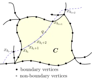
Proof: Letp = (v = x1, x2, . . . , xl= w) be a shortest path in G and let (xb1, xb2, . . . , xbj) be the subsequence of
all boundary vertices in p, i.e., 1 = b1 < · · · < bj = l
and there are no boundary vertices on p between xbi and
xbi+1. Hence p0= (xb1, xb2, . . . , xbj) is a path in BG. We
are going to estimate the length ofp0.
Leth = (xbi, xbi+1) be an edge of p0. Ifxbiandxbi+1are
from different components, then, by the definition of BG,
h is also an edge of G with the same weight as in BG. If
xbi andxbi+1 are from the same component C (Figure 1),
thenh corresponds to a subpath q = (xbi, xbi+1, . . . , xbi+1)
of p consisting of vertices from only C, by the assumption
that p0 contains all the boundary vertices of p. Hence, the
weight ofh and the length of q are the same. By induction
on the number of the edges of p0, p and p0 have the same
length, which implies that the distance betweenv and w in
BG is no greater than the distance between them in G. The reverse inequality is obtained in the same way, namely, by
showing that any path inBG can be transformed into a path
of the same length in G by replacing each virtual edge of
the former with the corresponding shortest path computed in Step 2. The claim follows.
This step presents no apparent parallelism, since only one task needs to be computed. This absence of parallelism at this step may be a major bottleneck for a coarse-grain parallel implementation as boundary graphs can be very
C
x
bix
bi+1x
bi−1x
bi+2x
bi+1x
bi+2boundary vertices
non-boundary vertices
q
Figure 1. Illustration to the proof of Lemma 1. The shaded region illustrates componentC with the subpath q = (xbi, xbi+1, . . . , xbi+1)
ofp inside it.
large. This issue can however be mitigated by applying our current algorithm recursively on the boundary graph. Boundary graphs are nevertheless denser than the original
graph with the addition of virtual edges at step1. Boundary
graphs are therefore less easily partitioned than input graphs - the number of edges cut per node for a given number of components will be higher.
E. Step 4: Distances between non-boundary vertices In Step 4 we compute distances where at least one vertex is non-boundary using the information computed in Steps 2 and 3. In order to compute the distance between
two non-boundary verticesvi andvj from (not necessarily
different) components Ci and Cj respectively, we need
to find boundary vertices bi and bj from components Ci
andCj, respectively, that minimize the sum dist2(vi, bi) + dist3(bi, bj) + dist2(bj, vj), where dist2 and dist3 are the distances computed in Step 2 and Step 3, respectively. By
our analysis above, dist3is the same as the distance inG, but
dist2 is not. We need therefore to prove that such a method
produces accurate distances inG.
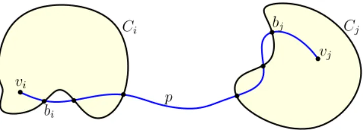
Lemma 2. Let vi and vj be two vertices from different
components Ci and Cj, respectively. Define Bi = Ci∩B,
Bj= Cj∩B, and
dist4(vi, vj) = min{dist2(vi, bi)+dist3(bi, bj)+dist2(bj, vj) | bi∈Bi, bj∈Bj}. (1) Then dist4(vi, vj) is equal to the distance in G between vi and vj.
Proof: Let p be a shortest path in G between vi and
vj. Since vi andvj belong to different components, thenp
will contain at least one vertex from Bi and at least one
vi bi bj vj Ci Cj p
Figure 2. Illustration to the proof of Lemma 2. Note that while in the figure bothviandvjare non-boundary, the proof does not make such an
assumption.
and bj be the last vertex on Bj (Figure 2). Letp1 be the
portion ofp between vi andbi,p2be the portion betweenbi
andbj, andp3 – the portion betweenbj andvj. Since any
subpath of a shortest path is also a shortest path between
the corresponding endpoints, p1 is a shortest path in G
between vi andbi, i.e., |p1| = distG(vi, bi). Moreover, by
the definition ofbi as the first boundary point ofCi on p,
p1 is entirely in Ci and hence |p1| = dist2(vi, bi). In the
same way one can prove that |p2| = dist2(bj, vj). Finally, |p3|= distG(bi, bj) = dist3(bi, bj) by Lemma 1. Hence |p| = |p1|+|p2|+|p3|= dist2(vi, bi)+dist3(bi, bj)+dist2(bj, vj).
By the definition of dist4(vi, vj) as a minimum over all
bi ∈ Bi, bj ∈ Bj, the last equality implies dist4(vi, vj) ≤ distG(vi, vj). But since dist4(vi, vj) is a length of a path between vi and vj, while distG(vi, vj) is the length of a shortest path, then dist4(vi, vj) ≥ distG(vi, vj). Combining the last two inequalities we infer that none of them can be a strict inequality, i.e., dist4(vi, vj) = distG(vi, vj).
Lemma 3. Letviandvjbe two vertices from componentCi.
Then distG(vi, vj) = min{dist2(vi, vj), dist4(vi, vj)}, where
dist4 is as defined in Lemma 2.
Proof:Consider the following two cases. Ifp leaves Ci,
thenp should cross the boundary Biat least twice. Definebi
andbjas the first and last vertex fromBionp. Then exactly
the same arguments as in Lemma 2 apply to the three paths into whichbi andbj divide p. In this case distG(vi, vj) = dist4(vi, vj). If p does not leave p, then Step 2 will compute
the accurate distance inG between vi andvj, and therefore
distG(vi, vj) = dist2(vi, vj).
The lemmas imply that the distances in G between all
pairs of vertices where at least one of the vertices is non-boundary can be computed by using (eq:step4). Since we
don’t know which pair (bi, bj) of boundary nodes
corre-sponds to the minimum in (eq:step4), we have to try all such pairs, resulting in total of |Bi||Bj| operations needed
for computing distG(vi, vj). For a graph with k components,
we need to compute the distances between pairs in any pair
of components; we therefore havek2−k independent tasks.
Components being of roughly equal sizes, these tasks also represent the same amount of computations. This step is
Part 1 Part 2 Part 3 Part 4 Part 3 3 1 3 1 Other vertices Boundary vertices Boundary Other Other vertices
Figure 3. Adjacency matrix after reordering of the vertices. Vertices from the same component are stored contiguously starting with boundary vertices (in red).
the most computationally intensive, but presents massive, already balanced, coarse-grain parallelism.
IV. METHOD
In this section, we first focus on how operations described in the previous section translate in terms of data structure. We then detail the two-level parallel aspect of our imple-mentation. We finally describe the current main memory bottleneck of our approach.
A. Relation to data structure
A simple way to represent a weighted graph is to use an adjacency matrix. For very large graphs however, such a memory intensive representation cannot be considered. Instead, large sparse graphs are stored using lists; sub-matrices, corresponding to sub-graphs, are extracted from these lists. For simplicity reasons, we can however assume that a large adjacency matrix representation is available and keep in mind that sub-matrix extraction operations are slightly more costly than they appear.
Partitioning the graph is performed using a k-way
parti-tioning routine from the METIS library [10]. Vertices are then reordered so that vertices belonging to a same com-ponent are numbered consecutively starting with boundary vertices - see Figure 3.
Diagonal matrices contain information about sub-graphs for each component; non-diagonal sub-matrices con-tain known shortest distances between components. Within each diagonal sub-matrix, the top left sub-matrix contains information about the sub-graph induces by boundary ver-tices of the component; the bottom right sub_matrix contains information about the sub-graph induced by non-boundary vertices of the component and the rest of the diagonal sub-matrix contains known shortest distances between boundary and non-boundary vertices.
For step 1, diagonal sub-matrices are extracted; a
Floyd-Warshall approach is then used to compute shortest dis-tances. The Floyd-Warshall algorithm guarantees that the total number of operations for a single matrix solely depends on the size of the matrix. Since all components of the graph
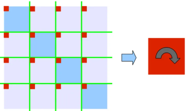
Figure 4. The boundary matrix, here in red, is scattered over the adjacency matrix. Step 2 consits in reconstituting the boundary matrix and computing shortest distances.
have roughly the same number of vertices, all diagonal sub-matrices represent roughly the same amount of operations.
For step2, the boundary matrix is extracted - see Figure 4.
We then apply the same algorithm recursively reducing the
number k of component at each iteration. Recursion stops
when k = 1.
For step3, we compute shortest distances between every
pair of distinct components. This process corresponds to
filling non-diagonal sub-matrices. For two componentsI and
J, filling the associated, I to J, non-diagonal sub-matrix requires information from three sub-matrices:
• the non-diagonal sub-matrix being filled. We are
partic-ularly interested in the part of the sub-matrix contain-ing shortest distances between boundary vertices from
component I to boundary vertices from component J.
• the diagonal sub-matrix corresponding to component
I - located in the same row as the non-diagonal sub-matrix being filled. We are particularly interested in the part of this diagonal sub-matrix that contains shortest
distances from any vertex of componentI to boundary
vertices.
• the diagonal sub-matrix corresponding to componentJ
- located in the same column as the non-diagonal sub-matrix being filled. We are particularly interested in the part of this diagonal sub-matrix that contains shortest
distances from boundary vertex of componentJ to any
vertex - see left of Figure 5.
Shortest distances from vertices from component I to
vertices from component J are obtained by multiplying
the three parts of sub-matrices - as shown on the right
of Figure 5 - where (+, ∗) operations are replaced with
(min, +) operations. B. Parallel implementation
Our implementation specifically targets large clusters of hybrid systems - possessing both a multicore CPU and
Part I Part J . . . . . . I J * * d b2,j d b1,b2 d i , b1
Figure 5. Computations associated to each non-diagonal sub-matrix uses data from 2 diagonal sub-matrices and part of the non-diagonal sub-matrix itself. Computations are similar to matrix multiplications.
manycore GPUs. This implementation exploits parallelism at two levels. At a coarse-grain level, large independent tasks - corresponding to computations of diagonal and non-daigonal sub-matrices - can be performed simultaneously on different nodes of a cluster. At a fine-grain level, each task is computed on a massively parallel GPU. Remaining CPU cores handle tasks that are not suited for GPUs: input/output file operations and communication with other nodes.
Coarse-grain parallelism: Steps1 and 3 of our algorithm
exhibit interesting parallel properties: a large number of
balanced, independent tasks;k tasks for step 1 and k2−k
for step 3. Using the MPI standard [11], these tasks are
distributed accross nodes of the cluster for simultaneous computations. One master node is in charge of reading the input graph file, calling the partitioning routine and sending tasks to a number of slave nodes equal to the number of available GPUs on the cluster. Depending on the cluster’s topology, the number of master and slave nodes will not match the number of physical nodes used on the cluster if each cluster node contains more than one GPU.
For step2, the large initial boundary matrix is computed
recursively using the same algorithm with decreasing values
for the numberk of components. The amount of independent
tasks therefore decreases with k, until a single, smaller
boundary matrix is obtained and computed by a single slave node.
Fine grain parallelism: Upon receiving a task from the
master node, each slave node then sends the corresponding data to its GPU for computations, retrieves results and send them back to the master node. Tasks are of two different kinds: diagonal workloads, which consist in computing shortest distances over a small subgraph, and non-diagonal workloads, which consist in multiplying three matrices.
Computations of diagonal workloads are implemented on the GPU using a blocked-recursive, Floyd-Warshall approach developped by [6] and adapted for non-power
of 2 matrices. Non-diagonal workloads require less
syn-chronization and can be implemented using a fast matrix-multiplication approach derived from [12] and adapted for (min, +) operations.
In this configuration, each physical node on the cluster makes use of as many CPU cores as there are available GPUs. If more CPU cores are available than GPUs, compu-tational power is still available. On slave nodes, remaining CPU cores are used for outputting final results to disk. On large clusters, communication between the master node and slave nodes can become a bottleneck, leaving slave nodes idle while waiting for the master node to be available. In order to increase the availability of the master node, a single CPU thread is used to initiate communications with slave nodes while remaining CPU cores handle the rest of the communications, updating data structures with temporary results and outputting final results to disk.
C. Memory limitations
For very large input graphs, memory usage becomes an issue. As stated previously, an entire adjacency matrix for the graph cannot be allocated; the graph is instead kept in memory as a list of edges, a much more memory-efficient representation. Even with this efficient representation, tem-porary sub-matrices need to be kept in memory: diagonal sub-matrices and boundary matrices. When recursively
com-puting step2, boundary matrices are output to files so as to
only keep a single boundary matrix in memory.
Final results for diagonal sub-matrices are only obtained
at the end of step2. As soon as final values for these diagonal
sub-matrices are obtained, they are output to files; only
relevant parts are kept in memory for step3; namely, parts of
these sub-matrices containing shortest distances from and to boundary vertices. Shortest distances between non-boundary vertices are thus discarded from main memory at the end of
step2.
The current limiting factor in terms of memory usage is the initial boundary matrix. The first boundary matrix has to fit in main CPU memory. Section V discusses ways to overcome this limitation. It is however probable that prohibitive run-times or an amount of results too large to process may become the limiting factor before main memory usage does.
V. RESULTS AND PERSPECTIVES
In this section, we compare our implementation to two parallel Dijkstra implementations. It is important to note that our implementation allows graphs with negative edges - but no negative cycles -, unlike Dijkstra based approaches.
In order to test our implementation, we generated random graphs with increasing numbers of vertices, ranging from 1024 to 1024k. These graphs, generated using the LEDA library [13], were made planar to ensure good partitioning properties.
Computations were run on a cluster of more than 300
computer nodes; each node is equipped with two NVIDIA C2090 GPUs, a 16 core Intel(R) Xeon(R) CPU E5-2670 0
@ 2.60GHz and32 GB of RAM. 1000 10000 100000 1000000 10000000 0,0E+0 5,0E+3 1,0E+4 1,5E+4 2,0E+4 2,5E+4 3,0E+4
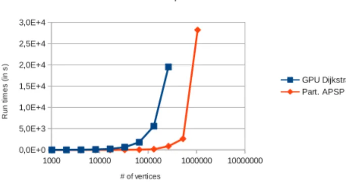
Run times with respect to # of vertices
GPU Dijkstra Part. APSP EM # of vertices R u n ti m e s ( in s )
Figure 6. Evolution of run times with respect to the number of vertices. Two implementations are compared: our implementation using external memory and the GPU Dijkstra implementation from [9]. Computations were run using two GPUs on a single cluster node.
Our implementation handles instances up to512k vertices
without using external memory. For the very last instance,
the use of external memory was required to fit in the 32
GB of main memory. We later refer to our implementation without using external memory as “Part. APSP no EM” and our implementation using external memory as “Part. APSP EM”.
The GPU Dijkstra implementation from [9] is, to the best of our knowledge, the only implementation that was
reported to solve APSP for graphs with up to1024k vertices;
we later refer to this implementation as “GPU Dijkstra”. This implementation parallelizes SSSP computations on a single computer using two GPUs and a multicore CPU. In order to compare this implementation to ours, we restricted computations of both implementations to using only two GPUs. Both implementations could therefore run on a single cluster node; no communication between nodes were there-fore required.
Figure 6 shows the runtimes for GPU Dijkstra and Part. APSP EM for graphs with numbers of vertices ranging from 1024 to 1024k using only two GPUs. GPU Dikstra could not
compute the last two instances - 512k and 1024k vertices
- within the 10 hour limit enforced on the cluster. We can see that our implementation is significantly faster than GPU Dijkstra.
Figure 7 shows the evolution of the speedup of our method without using external memory with respect to the number of GPUs used for the computations. Speedups are calculated using the run time obtained using only one GPU
as a reference. Computations were done for the512k vertex
instance using the Part. APSP no I/O implementation. We can see that coarse-grain parallelism is close to optimal up to
around 31 GPUs; almost no benefit can however be gained
from using more than about 63 GPUs. The reason for this
stagnation of the speedup above 63 GPUs is the saturation
of communication with the master node.
1 10 100 1000 1 10 100 1000 Speedup w.r.t. # of GPUs Ideal scaling Speedup # of GPUs S p e e d u p
Figure 7. Evolution of speedups with respect to the number of GPUs. The ideal scaling line is given as a reference.
parallelism approach that would relieve the master node of some of its communication. A work-stealing approach, for instance, would reduce the amount of communication required for the master node by decentralizing some of the memory transfers. A work-stealing approach is however difficult to implement, due to the two-sided communication scheme enforced by the MPI standard. [14] showed that such an efficient approach was nevertheless feasible. This issue could also be addressed by creating a hierarchy of master nodes; some computations would be redundant between the different master nodes handling the main data structure -but this would only represent a negligible fraction of the overall workload.
Figure 8 shows a comparison between our two implemen-tations and a distributed Dijkstra approach - later referred to
as CPU Dijkstra - for graphs ranging from 1024 to 1024k
vertices. The distributed Dijkstra approach was implemented by dynamically distributing SSSP computations for each vertex of the graph over every core of every available cluster node. The Dijkstra-based implementation used is that of the Boost C++ library [15]. This experiment is not intended
to compare directly the performances of 2 GPUs versus a
multicore CPU. Instead, we intend to show that our approach is competitive with a distributed Dijkstra approach given a fixed number of heterogeneous cluster nodes. The run times
presented in Figure 8 were obtained using64 cluster nodes.
We can see that our version using external memory obtains very similar run times to that of the distributed Dijkstra version, while allowing graphs with negative edges to be computed. Our version without external memory is however significantly faster.
REFERENCES
[1] E. W. Dijkstra, “A note on two problems in connexion with graphs,” Numerische mathematik, vol. 1, no. 1, pp. 269–271, 1959.
[2] J. Leskovec, D. Huttenlocher, and J. Kleinberg, “Predicting positive and negative links in online social networks,” in Proceedings of the 19th international conference on World
wide web. ACM, 2010, pp. 641–650.
1000 10000 100000 1000000 10000000 0 200 400 600 800 1000 1200 1400 1600
Run times w.r.t. # of vertices
Part. APSP EM CPU Dijkstra Part. APSP no EM # of vertices R u n ti m e s ( in s )
Figure 8. Evolution of run times with respect to the number of vertices. Three implementations are compared: our two implementations - with and without using external memory - and a distributed Dijkstra implementation referred to as CPU Dijkstra. All computations were run on 64 cluster nodes.
[3] V. Traag and J. Bruggeman, “Community detection in net-works with positive and negative links,” Physical Review E, vol. 80, no. 3, p. 036115, 2009.
[4] K. Inoue, A. Doncescu, and H. Nabeshima, “Hypothesizing about causal networks with positive and negative effects by meta-level abduction,” in Inductive Logic Programming. Springer, 2011, pp. 114–129.
[5] P. Harish and P. Narayanan, “Accelerating large graph al-gorithms on the gpu using cuda,” in High performance
computing–HiPC 2007. Springer, 2007, pp. 197–208.
[6] A. Buluç, J. R. Gilbert, and C. Budak, “Solving path problems on the gpu,” Parallel Computing, vol. 36, no. 5, pp. 241–253, 2010.
[7] T. Okuyama, F. Ino, and K. Hagihara, “A task parallel algorithm for finding all–pairs shortest paths using the gpu,” International Journal of High Performance Computing and Networking, vol. 7, no. 2, pp. 87–98, 2012.
[8] K. Matsumoto, N. Nakasato, and S. G. Sedukhin, “Blocked united algorithm for the all-pairs shortest paths problem on hybrid cpu-gpu systems,” IEICE TRANSACTIONS on Infor-mation and Systems, vol. 95, no. 12, pp. 2759–2768, 2012. [9] H. Ortega-Arranz, Y. Torres, D. R. Llanos, and A.
Gonzalez-Escribano, “The all-pair shortest-path problem in shared-memory heterogeneous systems,” 2013.
[10] G. Karypis and V. Kumar, “Multilevel k-way partitioning scheme for irregular graphs,” Journal of Parallel and Dis-tributed computing, vol. 48, no. 1, pp. 96–129, 1998. [11] M. Snir, S. W. Otto, D. W. Walker, J. Dongarra, and S.
Huss-Lederman, MPI: the complete reference. MIT press, 1995.
[12] V. Volkov, “Better performance at lower occupancy,” in Pro-ceedings of the GPU Technology Conference, GTC, vol. 10, 2010.
[13] K. Mehlhorn, S. Näher, and C. Uhrig, “Leda: A platform for combinatorial and geometric computing,” vol. 38, 1999.
[14] G. P. Pezzi, M. C. Cera, E. Mathias, and N. Maillard, “On-line scheduling of mpi-2 programs with hierarchical work stealing,” in Computer Architecture and High Performance Computing, 2007. SBAC-PAD 2007. 19th International
Sym-posium on. IEEE, 2007, pp. 247–254.
[15] B. Dawes, D. Abrahams, and R. Rivera, “Boost c++ libraries,” URL http://www. boost. org, vol. 35, p. 36, 2009.
VI. ACKNOWLEDGMENTS
This work was partially supported by the region of Brit-tany, France.