1 2 3 4 5 6 7 8 9 10 11
ASSESSING THE QUALITY OF ORIGIN-DESTINATION MATRICES 12
DERIVED FROM ACTIVITY/TRAVEL SURVEYS: 13
RESULTS FROM A MONTE CARLO EXPERIMENT 14
15 16 17
Mario Cools, Elke Moons, Geert Wets*
18 19
Transportation Research Institute
20 Hasselt University 21 Wetenschapspark 5, bus 6 22 BE-3590 Diepenbeek 23 Belgium 24 Fax.:+32(0)11 26 91 99 25 Tel.:+32(0)11 26 91{31, 26, 58} 26
Email: {mario.cools, elke.moons, geert.wets}@uhasselt.be
27 28 29 30 * Corresponding author 31 32 33 Number of words = 4,342 34 Number of Figures = 8 35 Number of Tables = 4 36
Words counted: 4,342 + 12*250 = 7,342 words
37 38
Revised paper submitted: November 13, 2009
39 40 41 42 43
ABSTRACT 1
2
To support policy makers combating travel-related externalities, quality data is required for the
3
design and management of transportation systems and policies. To this end, large amounts of
4
money have been spent on collecting household and person-based data. The main objective of
5
this paper is to assess the quality of origin-destination matrices derived from household
6
activity/travel surveys. To this purpose, a Monte Carlo experiment is set up to estimate the
7
precision of OD-matrices given different sampling rates. The Belgian 2001 census data,
8
containing work/school-related travel information for all 10,296,350 residents, are used for the
9
experiment. For different sampling rates, 2000 random stratified samples are drawn. For each
10
sample, three origin-destination-matrices are composed: one at municipality level, one at district
11
level, and one at provincial level. The correspondence between the samples and the population is
12
assessed by using the Mean Absolute Percentage Error (MAPE) and a censored version of the
13
MAPE (MCAPE). The results show that no accurate OD-matrices can be directly derived from
14
these surveys. Only when half of the population is queried, an acceptable OD-matrix is obtained
15
at provincial level. Therefore, it is recommended to use additional information to better grasp the
16
behavioral realism underlying destination choices and to collect information about particular
17
origin-destination pairs by means of vehicle intercept surveys. In addition, the results suggest
18
using the MCAPE next to traditional criteria to examine dissimilarities between different
OD-19
matrices. An important avenue for further research is the investigation of the effect of sampling
20
proportions on travel demand model outcomes.
21 22 23
1 BACKGROUND 1
2
In the modern cosmopolite society, travel is a cornerstone for human development, both for
3
personal and commercial reasons: travel is not only regarded as one of the boosting forces
4
behind economic growth, but is also seen as a social need providing people the opportunity for
5
self-fulfillment and relaxation. As a result of the continuous evolution of modern society (e.g.
6
urban sprawl, increasing female participation in labor, decline in traditional household
7
structures), transportation challenges have accrued and have become more complex (1).
8
Consequently, combating environmental (e.g. greenhouse-emissions such as CO2, methane,
9
NOx; noise, odor annoyance and acid precipitation), economic (e.g. use of nonrenewable energy
10
sources; and time lost due to congestion) and societal (e.g. health problems such as
11
cardiovascular and respiratory diseases; traffic casualties; community severance and loss of
12
community space) repercussions is a tremendous task (2).
13
To support policy makers in addressing these externalities, quality data are required for
14
the design and management of transportation systems and policies (3). To this end, during the
15
last four decades, large amounts of money have been spent on collecting household and
person-16
based data. For most metropolitan areas, the largest part of planning budgets (an estimated $7.4
17
million per year) was devoted to the conduct of household and person travel surveys (4). The
18
data collected by these surveys are used for a wide variety of applications, including traffic
19
forecasting, transportation planning and policy, and system monitoring (3).
20
The main objective of this paper is to assess the quality of origin-destination matrices
21
derived from travel surveys. Mark that origin-destination matrices are core components in both
22
traditional four-step and modern activity-based travel demand models. A sample size experiment
23
is set up to estimate the precision of the OD-matrices given different sampling rates. Thus, an
24
assessment of the appropriateness of travel surveys for deriving origin-destination relations can
25
be made. Note that different types of travel surveys exist: Cambridge Systematics (5)
26
distinguished seven different commonly used types of surveys (household activity/travel
27
surveys; vehicle intercept and external surveys; transit onboard surveys; commercial vehicle
28
surveys; workplace and establishment surveys; hotel/visitor surveys; and parking surveys). Each
29
of these survey types provides a unique perspective for input into travel demand models. In this
30
paper, the term ‘travel survey’ is confined to the first category, namely the household
31
activity/travel surveys.
32
In a household activity/travel survey, respondents are queried about their household
33
characteristics, the personal characteristics of the members of the household, and about recent
34
activity/travel experiences of some or all household members. For most regions, household
35
activity/travel surveys remain the best source of trip generation and distribution data, and
36
therefore, are an important building block for travel demand models. In addition to model
37
building purposes, these surveys are also used to poll specific target populations (such as transit
38
users and non-users), to assess the potential demand and level of public support for major
39
infrastructural projects, and to create a deeper understanding of travel behavior in the region (5).
40
For a more elaborate discussion concerning travel surveys the reader is referred to (3,5,6).
41
Recent trends in household travel surveys are discussed by Stopher and Greaves (7).
42
The remainder of this paper is organized as follows. Section 2 provides an extended
43
discussion on the set-up of the sample size experiment. The relationship between sampling rates
44
and the precision of a general statistic (i.e. the proportion of the commuting population) is
45
highlighted in the first part of Section 3. The second part of Section 3 provides the results and
corresponding discussion of the statistical analysis of the main sample size experiment. Finally,
1
some general conclusions will be formulated and avenues for further research indicated.
2 3
2 SET-UP OF THE SAMPLE SIZE EXPERIMENT 4
5
As mentioned in the introduction, the main goal of this paper is the assessment of the quality of
6
origin-destination matrices derived from household activity/travel surveys and, consequently,
7
providing an answer to the question of how large a sample size should be to provide accurate
8
OD-information in a region. To this end a Monte Carlo experiment is set up to estimate the
9
precision of the OD-matrices given different sampling rates. A Monte Carlo experiment involves
10
the use of random sampling techniques and computer simulation to obtain approximate solutions
11
to mathematical problems. It involves repeating a simulation process, using in each simulation a
12
particular set of values of random variables generated in accordance with their corresponding
13
probability distribution functions (8). A Monte Carlo experiment is a viable approach for
14
obtaining information about the sampling distribution of a statistic (in this study the precision of
15
an origin-destination matrix) of which a theoretical sampling distribution may not be available
16
due to the complexity. Monte Carlo simulation is generally suitable for addressing questions
17
related to sampling distribution, especially when a) the theoretical assumptions of the statistical
18
theory are violated; b) the theory about the statistic of interest is weak; or c) no theory exists
19
about the statistic of interest (9). The latter is the case in this study (i.e. the precision of
OD-20
matrices given different sampling rates).
21
The Monte Carlo experiment reported in this paper focuses on commuting (i.e. work and
22
school related) trips made in Belgium. The 2001 census data will be used for the experiment. In
23
particular, the census queried information about the departure and arrival times and locations of
24
work/school trips (when applicable) for all 10,296,350 residents. For different sampling rates,
25
ranging from one (the full population) to a millionth, 2,000 random stratified samples were
26
drawn (2,000 for each sampling rate). Note that this number of samples is common in
27
transportation oriented simulation experiments (e.g. 10,11). To ensure that the persons in the
28
samples were geographically distributed in the country, the sample was stratified by
29
geographical area: three nested stratification levels were taken into account, namely province,
30
district and municipality. The sample was proportionately allocated to the strata. In other words,
31
the sample in each stratum was selected with the same probabilities of selection (12).
32
For each sample, the proportion of persons making commuting trips was calculated, and
33
three corresponding (morning commute) origin-destination-matrices (OD-matrices) were
34
composed: one OD-matrix on municipality level (589 by 589 matrix), one OD-matrix on district
35
level (43 by 43 matrix), and one on provincial level (11 by 11 matrix). A side-note has to be
36
made for the latter OD-matrix: actually there are only 10 provinces in Belgium, but the Brussels
37
metropolitan capital area (accounting for about 1/10 of the entire population) was treated as a
38
separate province. The correspondence of the sample proportion and sample OD-matrices with
39
the population (census) proportion and OD-matrices was then tabulated.
40
The correspondence between the sample and the population is assessed by using the
41
Mean Absolute Percentage Error (MAPE) and an accommodated version of the MAPE. The
42
MAPE is the mean of the Absolute Percentage Errors (APE) and is calculated by:
43
ij ij
i j
MAPE =
∑∑
APE N, with ij ij ij 100 ij A E APE A − = × , 44where Aij is the population count for the morning commute from origin i to destination j, Eij the
1
sample count (scaled up to population level) for this morning commute, and N the total number
2
of origin-destination cells. Despite its widespread use, the MAPE has several disadvantages.
3
Armstrong and Collopy (13) for instance, argued that the MAPE is bounded on the low side by
4
an error of 100% (origin-destination counts are all positive integers), but there is no bound on
5
the high side. In response to this comment, Makridakis (14) proposed a modified MAPE
6
(MDAPE), which is often referred to as SAPE (smoothed absolute percentage error) or SMAPE
7
(symmetric mean absolute percentage error). This modified MAPE (MDMAPE) is given by:
8
ij ij
i j
MDMAPE =
∑∑
MDAPE N, where(
)
2 100 ij ij ij ij ij A E MDAPE A E − = × + . 9Although this modification accommodates the above described problem, it treats large positive
10
and negative errors very differently (15). Therefore, in this paper, a new modification of the
11
MAPE is proposed, named the Mean Censored Absolute Percentage Error (MCAPE). This new
12
statistic takes into account the above described comments by limiting the positive values to a
13
maximum of 100. Mathematically, the MCAPE is given by the following formula:
14
ij ij
i j
MCAPE =
∑∑
CAPE N, where ij min 100, ij ij 100ij A E CAPE A − = × . 15
When Aij in the above formulae would be equal to zero, the different criteria would be
16
undefined. This has been remedied by equalizing the APEij, MDAPEij and CAPEij to zero in
17
these occasions. After all, when the true population count equals zero (no person in the full
18
population corresponds to the considered origin-destination pair) the up-scaled sample count
19
also equals zero, and thus the true zero is correctly estimated.
20
The correspondence between the sample proportion (p) of persons making commuting
21
trips and population proportion (π) is calculated by simply calculating the Absolute Percentage
22 Error (APE): 23 100 p APE π π − = × . 24
No accommodation of this APE was required, as the population proportion (π) was equal to
25
62.59 percent, and consequentially the APE could not exceed 100.
26
To recapitulate, for each sampling rate, 2000 MAPE values and MCAPE values are
27
calculated for the OD-matrix on municipality level, for the OD-matrix on district level, and for
28
the OD-matrix on province level. In addition 2000 APE values are computed for the commuting
29
proportion. For each of these sets of 2000 values, the 2.5th percentile, the 5th percentile, the 95th
30
percentile and the 97.5th percentile was calculated. The kth percentile is that value x such that the
31
probability that an observation drawn at random from the population is smaller than x, equals k
32
percent (16). The 2.5th percentile and 97.5th percentile are used to construct the 95% percentile
33
interval which will be illustrated graphically as lower and upper bounds for the median. The 5th
34
percentile and 95th percentile will be displayed in the corresponding tables because one is most
35
often only interested in the one-sided alternative. In addition, the median (the 50th percentile)
36
and the arithmetic mean are also computed.
37
To guarantee that the Monte Carlo experiment is really estimating the precision of the
38
OD-matrices in function of different sample rates, rather than in function of other (unobserved)
39
effects, one could take a look at the different sources of errors and biases in surveys. Groves (17)
40
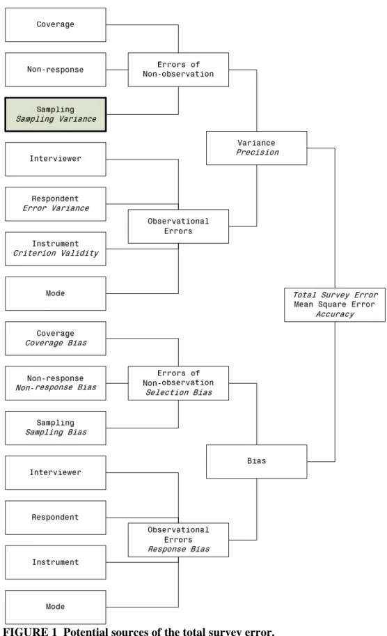
distinguished different sources of inaccuracy in surveys, of which an overview is given in Figure
1. Since in this experiment the true population values are known, and samples are drawn under
1
ideal circumstances (no response bias, no selection bias, no observation errors, no non-response
2
and perfect coverage), the resulting variations in the experiment are only a consequence of the
3
sampling variance (indicated with a gray box, framed with a tick black line in Figure 1). Thus, as
4
intended, the relationship between different sample sizes and the precision/accuracy (sample
5
variance) of the quantities under study are investigated.
6 7
1
FIGURE 1 Potential sources of the total survey error. 2
3 RESULTS 1
2
3.1 Proportion of the Commuting Population 3
4
Before elaborating on the quality of OD-matrices in the second part of this Section, in this first
5
part, an assessment of the appropriateness of travel surveys for deriving traditional indices, such
6
as the mean number of trips made or the mean number of activities performed by
7
individuals/households, or the proportion of the population making work/school-related trips, the
8
latter being subject of the Monte Carlo experiment, is made. For traditional indices such as the
9
mean number of trips made / activities performed by individuals/households, classical sample
10
size calculations can be used to determine optimal sample sizes. Cools et al. (18), for instance,
11
calculated the required number of households for a household activity survey using the
12 following formula: 13
(
)
2 2 1 z p p n md − ≥ , 14where n equals the sample size, p the sample (survey) proportion, md the maximal deviation and
15
z the z-value of the desired confidence interval. For the ‘safest’ case (i.e. p = 0.5), a maximal
16
deviation of 2% and a confidence level of 95% would require a minimum of at least 2,401
17
households. This example illustrates that for aggregate indices, such as the proportion of the
18
commuting population, a clear theory exists and Monte Carlo simulation is not per se required.
19
Notwithstanding, an investigation of the relationship between sampling rates and precision
20
(sample variance) is still valuable, and especially contributes to the literature when the focus is
21
turned to the different percentiles that are examined.
22
Results from the Monte Carlo experiment for the proportion of commuters in the
23
population are graphically displayed in Figure 2 and numerically represented in Table 1.
24 25
26
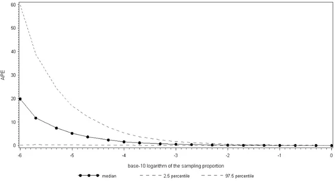
FIGURE 2 Relationship between absolute percentage error and sampling rate for 27
commuting proportion. 28
Figure 2 shows a clear relationship between the Absolute Percentage Error (APE) and the
1
sampling proportion. As expected, the additional improvement in precision decreases as the
2
sampling rate increases: for instance the increase in precision (decrease in APE) from a sampling
3
rate of one millionth (base-10 logarithm of the sampling proportion equals minus 6) to one
4
hundred-thousandth (base-10 logarithm equals minus 5) is considerably larger than the increase
5
in precision from a sampling rate of one thousand to one hundred. This is especially so for the
6
upper bound of the 95% percentile interval (97.5th percentile).
7 8
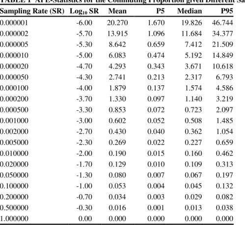
TABLE 1 APE-Statistics for the Commuting Proportion given Different Sampling Rates1
9
Sampling Rate (SR) Log10 SR Mean P5 Median P95
0.000001 -6.00 20.270 1.670 19.826 46.744 0.000002 -5.70 13.915 1.096 11.684 34.377 0.000005 -5.30 8.642 0.659 7.412 21.509 0.000010 -5.00 6.083 0.474 5.192 14.849 0.000020 -4.70 4.293 0.343 3.671 10.618 0.000050 -4.30 2.741 0.213 2.317 6.793 0.000100 -4.00 1.879 0.137 1.574 4.586 0.000200 -3.70 1.330 0.097 1.140 3.219 0.000500 -3.30 0.853 0.072 0.723 2.097 0.001000 -3.00 0.602 0.052 0.508 1.485 0.002000 -2.70 0.430 0.040 0.362 1.054 0.005000 -2.30 0.269 0.022 0.227 0.659 0.010000 -2.00 0.190 0.015 0.160 0.462 0.020000 -1.70 0.129 0.010 0.109 0.313 0.050000 -1.30 0.080 0.007 0.067 0.197 0.100000 -1.00 0.053 0.004 0.045 0.132 0.200000 -0.70 0.034 0.003 0.029 0.082 0.500000 -0.30 0.016 0.001 0.013 0.038 1.000000 0.00 0.000 0.000 0.000 0.000 1
‘P’ stands for the percentile, e.g. P5 stands for the 5th percentile. 10
11
The results also show that when the full population is sampled, an absolute precision is
12
obtained (absence of all variation). By definition this result should be obtained. When an average
13
deviation of 5 percent is considered acceptable, a sample rate between 1 and 2
hundred-14
thousandth is required (5 percent lies between the mean values 4.293 and 6.083). On the other
15
hand, from the median value one could conclude that in 50% of the cases the maximal deviation
16
(APE) is smaller than 5.192 percent. A more cautions approach entails the use of the 95th
17
percentiles. Suppose that only 5% of the cases the APE was allowed to exceed 2, then a
18
sampling rate of about 5 ten-thousandth would be required, which roughly corresponds to
19 sampling 5000 persons. 20 21 22 23
3.2 Precision of Origin-Destination Matrices 1
2
In this part of the result section, an assessment of the appropriateness of household
3
activity/travel surveys for deriving OD-matrices is made. Recall that a Monte Carlo simulation is
4
particularly suitable for addressing the questions concerning the distribution of the precision of
5
these OD-matrices, as no real theoretical background of this distribution exists. First, attention
6
will be paid to OD-matrices at municipality level. Afterwards, the focus is laid on OD-matrices
7
at district and provincial level.
8 9
3.2.1 OD-Matrices at Municipality Level
10 11
Before expanding on the results of the Monte Carlo experiment, it is important to mention that
12
the true OD-matrix (OD-matrix composed from the full population) is a very large and sparse
13
matrix: of the 346,921 origin-destination pairs (589 times 589), 77.8% are cells. As
zero-14
cells in the full population are by definition correctly predicted by taking a sample from this
15
population, the actual overall precision is significantly boosted by the sparseness of the true
OD-16
matrix. Therefore, the decision was made to present the results based on the 76,882
non-zero-17
cells. To derive the values that include the zero-cells, one only needs to divide the MAPE and
18
MCAPE values by 4.512 (= all cells / (all cells – zero-cells)).
19 20
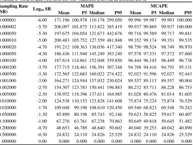
TABLE 2 MAPE and MCAPE for OD-Matrices Derived at Municipality Level
21
MAPE MCAPE Sampling Rate
(SR) Log10 SR Mean P5 Median P95 Mean P5 Median P95
0.000001 -6.00 205.996 100.902 115.559 753.493 100.000 100.000 100.000 100.000 0.000002 -5.70 200.992 102.528 129.575 754.266 100.000 100.000 100.000 100.000 0.000050 -5.30 199.861 109.279 155.540 431.119 99.999 99.998 99.999 100.000 0.000010 -5.00 199.089 116.768 175.588 352.896 99.997 99.995 99.997 99.999 0.000020 -4.70 198.647 127.682 187.707 304.125 99.994 99.992 99.994 99.996 0.000050 -4.30 198.338 148.261 194.723 259.440 99.977 99.972 99.977 99.981 0.000100 -4.00 199.452 160.661 198.325 243.313 99.927 99.919 99.927 99.936 0.000200 -3.70 197.459 170.778 196.746 226.279 99.784 99.769 99.784 99.798 0.000500 -3.30 195.930 178.611 195.344 215.156 99.414 99.391 99.414 99.437 0.001000 -3.00 193.624 181.284 193.511 206.508 98.999 98.973 98.999 99.026 0.002000 -2.70 190.182 181.664 189.982 199.411 98.393 98.360 98.392 98.427 0.005000 -2.30 183.425 177.916 183.465 188.907 97.033 96.990 97.033 97.077 0.010000 -2.00 175.654 171.907 175.659 179.551 95.352 95.298 95.353 95.407 0.020000 -1.70 164.993 162.373 165.044 167.739 92.797 92.730 92.798 92.865 0.050000 -1.30 145.263 143.745 145.271 146.836 87.514 87.424 87.515 87.598 0.100000 -1.00 124.970 124.078 124.960 125.866 81.369 81.273 81.369 81.469 0.200000 -0.70 99.172 98.724 99.169 99.631 72.293 72.193 72.294 72.392 0.500000 -0.30 54.108 54.089 54.108 54.128 54.108 54.089 54.108 54.128 1.000000 0.00 0.000 0.000 0.000 0.000 0.000 0.000 0.000 0.000 22
Inspection of Table 2 immediately reveals that no accurate OD-matrices are obtained at
1
municipality level, even if zero-cells are taken into account: a survey that would query half of
2
the population still would have an average absolute percentage error of 11.99 percent when
zero-3
cells are included and correspondingly of 54.11 % when only the actual predictions
(non-zero-4
cells) are taken into account. This clearly indicates that the direct derivation of origin-destination
5
matrices from household activity/travel surveys should be avoided. Notwithstanding,
origin-6
destination matrices derived from household activity/travel surveys are very valuable: even a
7
simple gravity model with the inverse squared distance as deterrence function, taking into
8
account the productions and attractions derived from the surveys, already results in a clear
9
improvement of the OD-matrices. This is certainly a plea for travel demand models that
10
incorporate the behavioral underpinnings of destination choices (activity location choices) given
11
a certain origin, like for instance models that make use of space-time prisms, e.g. (19), and
12
models that combine data from different sources, such as data integration tools, e.g. (20). In
13
addition, OD-matrices derived from travel surveys form a good basis for OD-matrices derived
14
from traffic counts: as multiple OD-matrices can be derived from the same set of traffic counts,
15
OD-matrices derived from travel surveys provide a good basis for constraining the matrices
16
derived from traffic counts (21). A thorough look at Table 2 also reveals that when half the
17
population is sampled, the values for the MAPE and MCAPE are the same. This can be
18
explained by the fact that when using half of the population none of the 2000 samples has a
19
MAPE higher than 1.
20
When the general tendency of the precision of the OD-matrices derived from travel
21
surveys is discussed, Figures 3 and 4 provide a clear insight in the relationship between the
22
precision and the sampling rate. From Figure 3 one can clearly see that the median MAPE first
23
increases when samples are becoming larger, and then starts to decrease. The increase in median
24
MAPE for the smallest sampling rates can be accounted for by the fact that on average more
25
cells are seriously overestimated, whereas the maximum underestimations are bounded by
26
100%. This effect is filtered out by using the MCAPE, as can be seen from Figure 4; a clear
27
decreasing relationship is visible here. Next to the difference in relationships between the MAPE
28
and MCAPE, one could also observe a clear difference between the percentile interval for the
29
MAPE and the percentile interval for the MCAPE. By condensing the APE to a maximum of
30
one (i.e. the CAPE), almost all variability around the median value is filtered out: the 2.5th and
31
97.5th percentiles almost coincide with the median values in case of the MCAPE.
32
When this decreasing pattern of the MCAPE (Figure 4) is compared to the one of the
33
proportions (Figure 2), a clear contrast in the tendency can be seen: while the pattern for
34
proportion is a convex decreasing function, for the OD-matrices this is a concave decreasing
35
function. This difference in pattern, as well as the difference in precision, can be explained by
36
the fact that proportions are aggregate indices, and that surveys are extremely suitable for
37
capturing these aggregate figures, while in OD-matrices all individual information is used.
38 39 40
M A P E ( b a s e d o n a ll n o n -z e ro c e lls ) 0 100 200 300 400 500 600 700 800 900 1000 1100 1200 1300 1400 1500
base-10 logarithm of the sampling proportion
-6 -5 -4 -3 -2 -1 0
median 2.5-th percentile 97.5-th percentile
1
FIGURE 3 Relationship between MAPE and base-10 logarithm of the sampling rate. 2 3 M C A P E ( b a s e d o n a ll n o n -z e ro c e lls ) 0 10 20 30 40 50 60 70 80 90 100
base-10 logarithm of the sampling proportion
-6 -5 -4 -3 -2 -1 0
median 2.5-th percentile 97.5-th percentile
4
FIGURE 4 Relationship between MCAPE and base-10 logarithm of the sampling rate. 5
6
3.2.2 OD-Matrices at District Level
7 8
Similar to the true OD-matrix at municipality level, the true OD-matrix at district level (43 by
9
43) comprises a non-negligible amount of zero-cells. Nonetheless, the number of non-zero-cells
10
is considerably smaller: 10.4% of the 1,849 origin-destination pairs are zero-cells. Recall that
11
zero-cells in the full population are by definition correctly predicted by taking a sample from this
population. Therefore, similar to the previous paragraph, the results are based on the 1,657
non-1
zero-cells. The values that include the zero-cells can be calculated by dividing the MAPE and
2
MCAPE values by 1.116.
3
A thorough look at Table 3 shows that also at district level no accurate OD-matrices can
4
be derived. Even if zero-cells are included in the calculations, surveying half of the population
5
would result in an average absolute percentage error of 22.25 percent (24.832 divided by 1.116).
6
When compared to the results of OD-matrices derived at municipality level, the results including
7
the zero-cells are worse at district level than at municipality level (an average MAPE of 22.25
8
percent versus one of 11.99 percent). This is due to the fact that at municipality level a much
9
larger share (77.8 percent versus 10.4 percent) of zero-cells is automatically correctly predicted.
10
In contrast, when the results of only the non-zero-cells are compared, the precision of the
OD-11
matrices derived at district level is higher than the precision of the OD-matrices derived at
12
municipality level. This result confirms that predictions on a more aggregate level are more
13
precise.
14 15
TABLE 3 MAPE and MCAPE for OD-Matrices Derived at District Level 16
MAPE MCAPE Sampling Rate
(SR) Log10 SR Mean P5 Median P95 Mean P5 Median P95
0.000001 -6.00 171.196 100.978 110.178 299.050 99.996 99.987 99.993 100.000 0.000002 -5.70 206.097 101.875 113.822 385.419 99.937 99.869 99.937 100.000 0.000050 -5.30 197.675 104.054 121.673 442.676 99.716 99.589 99.717 99.841 0.000010 -5.00 200.483 105.752 127.559 481.848 99.352 99.174 99.351 99.535 0.000020 -4.70 191.212 108.363 136.036 417.340 98.750 98.524 98.749 98.970 0.000050 -4.30 186.436 111.940 145.249 383.240 97.578 97.331 97.572 97.860 0.000100 -4.00 187.614 114.861 152.048 359.850 96.444 96.145 96.449 96.738 0.000200 -3.70 177.715 118.461 156.391 307.348 94.788 94.416 94.791 95.131 0.000500 -3.30 172.565 122.683 160.022 274.422 92.023 91.596 92.027 92.443 0.001000 -3.00 164.271 124.944 157.032 230.024 89.557 89.113 89.557 90.004 0.002000 -2.70 154.307 123.783 150.441 196.883 86.232 85.711 86.228 86.753 0.005000 -2.30 138.952 118.396 137.611 164.985 81.028 80.476 81.014 81.605 0.010000 -2.00 124.538 110.153 123.828 141.608 75.874 75.224 75.874 76.529 0.020000 -1.70 109.048 99.198 108.610 120.450 69.540 68.823 69.548 70.242 0.050000 -1.30 85.890 80.198 85.743 92.146 59.623 58.825 59.617 60.407 0.100000 -1.00 67.276 63.761 67.238 70.863 50.649 49.818 50.645 51.482 0.200000 -0.70 48.653 46.789 48.640 50.602 40.040 39.253 40.042 40.890 0.500000 -0.30 24.832 24.110 24.826 25.529 24.832 24.110 24.826 25.529 1.000000 0.00 0.000 0.000 0.000 0.000 0.000 0.000 0.000 0.000 17
A visual representation of the relationship between the precision of the OD-matrices
18
derived at district level and the sampling rate is provided in Figures 5 and 6. Inspection of Figure
19
5 reveals a pattern very similar to the one observed in Figure 3: the MAPE first increases when
20
samples are becoming larger, and then starts to decrease. Recall that the increase in median
21
MAPE for the smallest sampling rates can be accounted for by the fact that more cells are
seriously overestimated on average, while the maximum underestimations are bounded by
1
100%. By analogy with the results at municipality level, this effect is filtered out by using the
2
MCAPE, as could be noticed from Figure 6. Moreover, the relationship between the MCAPE
3
and sampling proportion is a concave decreasing function, similar to the relationship between the
4
MCAPE and sampling rate at municipality level.
5 6 M A P E ( b a s e d o n a ll n o n -z e ro c e lls ) 0 100 200 300 400 500 600 700 800 900
base-10 logarithm of the sampling proportion
-6 -5 -4 -3 -2 -1 0
median 2.5-th percentile 97.5-th percentile
7
FIGURE 5 Relationship between MAPE and base-10 logarithm of the sampling rate. 8 9 M C A P E ( b a s e d o n a ll n o n -z e ro c e lls ) 0 10 20 30 40 50 60 70 80 90 100
base-10 logarithm of the sampling proportion
-6 -5 -4 -3 -2 -1 0
median 2.5-th percentile 97.5-th percentile
10
FIGURE 6 Relationship between MCAPE and base-10 logarithm of the sampling rate. 11
3.2.3 OD-Matrices at Provincial Level
1 2
In contrast to the true OD-matrices at municipality and district level, the true OD-matrix at
3
provincial level (11 by 11) only comprises non-zero-cells. Examination of Table 4 reveals that at
4
provincial level, barely any accurate OD-matrices can be derived. Nonetheless, in contrast to the
5
results at municipality and district level, for the largest sample sizes acceptable results are
6
obtained: sampling half of the population would result in an average absolute percentage error of
7
3.4 percent, and surveying one fifth of the population results in an average absolute percentage
8
error of 7.4%. Results from Table 4, also confirm that predictions related with a more aggregate
9
level are more precise. Notwithstanding, results at provincial level confirm the finding unraveled
10
at the lower levels (municipality and district) that the direct derivation of origin-destination
11
matrices from household activity/travel surveys should be avoided.
12 13
TABLE 4 MAPE and MCAPE for OD-Matrices Derived at Provincial Level 14
MAPE MCAPE Sampling Rate
(SR) Log10 SR Mean P5 Median P95 Mean P5 Median P95
0.000001 -6.00 176.769 99.263 107.557 394.608 99.063 98.121 99.098 100.000 0.000002 -5.70 203.155 97.373 116.674 433.429 97.457 96.026 97.482 98.892 0.000050 -5.30 181.113 96.627 126.086 350.822 95.265 93.815 95.268 96.704 0.000010 -5.00 168.445 98.339 127.604 348.163 93.433 92.038 93.444 94.797 0.000020 -4.70 168.536 99.464 128.362 360.363 91.485 90.201 91.460 92.835 0.000050 -4.30 151.833 95.531 121.858 311.175 86.839 84.890 86.849 88.801 0.000100 -4.00 139.293 89.910 117.180 260.735 81.456 78.907 81.492 83.867 0.000200 -3.70 122.260 83.171 109.350 199.592 75.496 72.706 75.491 78.216 0.000500 -3.30 102.579 73.950 95.857 153.082 66.131 63.291 66.100 68.976 0.001000 -3.00 86.550 65.717 82.586 121.220 58.695 55.863 58.703 61.425 0.002000 -2.70 70.179 55.819 67.913 91.566 50.581 47.480 50.567 53.506 0.005000 -2.30 50.419 42.091 49.683 61.219 40.069 37.270 40.045 42.948 0.010000 -2.00 37.062 31.187 36.759 44.062 31.583 28.460 31.522 34.604 0.020000 -1.70 26.160 22.031 25.987 30.902 23.833 20.970 23.816 26.754 0.050000 -1.30 16.138 13.530 16.044 19.084 15.566 13.331 15.566 17.840 0.100000 -1.00 11.165 9.297 11.150 13.148 11.018 9.271 11.021 12.841 0.200000 -0.70 7.417 6.252 7.374 8.784 7.404 6.243 7.370 8.721 0.500000 -0.30 3.449 2.903 3.440 4.050 3.449 2.903 3.440 4.050 1.000000 0.00 0.000 0.000 0.000 0.000 0.000 0.000 0.000 0.000 15
The visualization of the relationship between the precision of the OD-matrices derived at
16
provincial level and the sampling proportion is shown in Figures 7 and 8. Analogous to the
17
relationships between the sample rate and the precision of the OD-matrices at municipality and
18
district level, the MAPE first increases when samples are becoming larger, and then starts to
19
decrease (Figure 7). Again, the use of the MCAPE filters out this effect. In contrast to the results
20
at municipality and district level, the relationship between the precision and the MCAPE reveals
21
an s-shaped decreasing function: for the smallest sampling rates the relationship is concavely
decreasing, similar to the OD-matrices at municipality and district level; but for the larger
1
sampling rates the relationship is a convex decreasing function. Moreover, the 95 percentile
2
interval is much wider than for the OD-matrices at less aggregated levels. The most important
3
reasons for this are the degree of sparseness and size of the matrix: for the less aggregate levels
4
(municipality and district level), a lot of the variability of the precision is taken away by the
5
large amounts of (zero-)cells.
6 7 M A P E ( b a s e d o n a ll c e lls ) 0 100 200 300 400 500 600 700 800
base-10 logarithm of the sampling proportion
-6 -5 -4 -3 -2 -1 0
median 2.5-th percentile 97.5-th percentile
8
FIGURE 7 Relationship between MAPE and base-10 logarithm of the sampling rate. 9 10 M C A P E ( b a s e d o n a ll c e lls ) 0 10 20 30 40 50 60 70 80 90 100
base-10 logarithm of the sampling proportion
-6 -5 -4 -3 -2 -1 0
median 2.5-th percentile 97.5-th percentile
11
FIGURE 8 Relationship between MCAPE and base-10 logarithm of the sampling rate. 12
4 CONCLUSIONS 1
2
In this paper, an assessment of the quality of origin-destination matrices derived from household
3
activity/travel surveys was made. The results showed that no accurate OD-matrices can be
4
directly derived from these surveys. Only when half of the population is queried, an acceptable
5
OD-matrix is obtained at provincial level. Therefore, it is recommended to use additional
6
information to better grasp the behavioral realism underlying destination choices. This is
7
certainly a plea for travel demand models that incorporate the behavioral underpinnings of
8
destination choices (activity location choices) given a certain origin. Moreover, matrix
9
calibration techniques could seriously improve the quality of the matrices derived from these
10
household activity/travel surveys. In addition, it is recommended to collect information about
11
particular origin-destination pairs by means of vehicle intercept surveys rather than household
12
activity/travel surveys, as these vehicle intercept surveys are tailored for collecting specific
13
origin-destination data. Mark that the results presented in this paper do not negate the value of
14
travel surveys as was shown in the example of deriving the commuting population, but indicate
15
that sophistication is needed in the manner in which the data are employed.
16
A second important finding in this paper is that traditional methods to assess the
17
comparability of two origin-destination matrices could be enhanced: the MCAPE index that was
18
proposed has clear advantages over the traditional indices. The most important advantage being
19
the fact that the MCAPE filters out the noise created by the asymmetry of the traditional criteria.
20
Therefore, when dissimilarities between different OD-matrices are investigated, the use of the
21
MCAPE index next to traditional criteria is highly recommended.
22
An important avenue for further research is the investigation of the relationship between
23
the variability in the outcomes of travel demand models and underlying survey data.
24
Triangulation of both travel demand modeling and small area estimation models could prove to a
25
pathway for success. An empirical investigation of the effect of sampling proportions in
26
household activity/travel surveys on final model outcomes would further illuminate the quest for
27
optimal sample sizes. A thorough examination of the minimum required sampling rate of a
28
household travel survey such that trip distribution models (e.g. a gravity model) could help fill in
29
the full trip table certainly is an important step in further analyses. Model complexity and
30
computability will certainly be key challenges in this pursuit.
31 32
5 ACKNOWLEDGEMENTS 33
34
The authors would like to thank Katrien Declerq for her advice on the implementation of the
35 experiment. 36 37 6 REFERENCES 38 39
(1) Haustein, S., and M. Hunecke. Reduced use of environmentally friendly modes of
40
transportation caused by perceived mobility necessities: an extension of the theory of
41
planned behavior. Journal of Applied Social Psychology, Vol. 37, No. 8, 2007, pp.
1856-42
1883.
43 44
(2) Steg, L. Can public transport compete with the private car. IATSS Research, Vol. 27, No. 2,
45
2003, pp. 27-35.
1
(3) TRB Committee on Travel Survey Methods. The On-Line Travel Survey Manual: A
2
Dynamic Document for Transportation Professionals. Provided by the Members and
3
Friends of the Transportation Research Board’s Travel Survey Methods Committee
4
(ABJ40), Washington, D.C., 2009. http://trbtsm.wiki.zoho.com. Accessed July 22, 2009.
5 6
(4) Stopher, P., R. Alsnih, C. Wilmot, C. Stecher, J. Pratt, J. Zmud, W. Mix, M. Freedman, K.
7
Axhausen, M. Lee-Gosselin, A. Pisarski, and W. Brög. Standardized Procedures for
8
Personal Travel Surveys. National Cooperative Highway Research Program Report 571.
9
Transportation Research Board, Washington, 2008.
10 11
(5) Cambridge Systematics. Travel Survey Manual. Prepared for U.S. Department of
12
Transportation and the U.S. Environmental Protection Agency. Travel Model Improvement
13
Program (TMIP), Washington, D.C., 1996.
14 15
(6) Tourangeau, R., M. Zimowski, and R. Ghadialy. An Introduction to Panel Surveys in
16
Transportation Studies. Report DOT-T-84, Prepared for the Federal Highway
17
Administration. National Opinion Research Center, Chicago, I.L., 1997.
18 19
(7) Stopher, P.R., and S.P. Greaves. Household travel surveys: Where are we going?
20
Transportation Research Part A: Policy and Practice, Vol. 41, No. 5, 2007, pp. 33-40.
21 22
(8) Rubinstein, R.Y. Simulation and the Monte Carlo Method. John Wiley and Sons, Inc., New
23
York, 1981.
24 25
(9) Fan, X., A. Felsővályi, S.A. Sivo, and S.C. Keenan. SAS® for Monte Carlo Studies: A
26
Guide for Quantitative Researchers. SAS Institute. Cary, N.C., 2000.
27 28
(10) Patel, A., and M. Thompson. Consideration and Characterization of Pavement
29
Construction Variability. In Transportation Research Record: Journal of the
30
Transportation Research Board, No. 1632, Transportation Research Board of the National
31
Academies, Washington, D.C., 1998, pp. 40-50.
32 33
(11) Awasthi, A., S.S. Chauhan, S.K. Goyal, and J.-M. Proth. Supplier selection problem for a
34
single manufacturing unit under stochastic demand. International Journal of Production
35
Economics, Vol. 117, No. 1, 2009, pp. 229-233.
36 37
(12) Groves, R.M., F.J. Fowler, M. Couper, J.M. Lepkowski, E. Singer, and R. Tourangeau.
38
Survey Methodology. John Wiley and Sons, Inc., Hoboken, N.J., 2004.
39 40
(13) Armstrong, J.S., and F. Collopy. Error measures for generalizing about forecasting
41
methods: empirical comparisons. International Journal of Forecasting, Vol. 8, No. 1,
42
1992, pp. 69–80.
43 44
(14) Makridakis, S. Accuracy measures: theoretical and practical concerns. International
45
Journal of Forecasting, Vol. 9, No. 4, 1993, pp. 527-529.
1
(15) Goodwin, P., and R. Lawton. On the asymmetry of the symmetric MAPE. International
2
Journal of Forecasting, Vol. 15, No. 4., 1999, pp. 405-408.
3 4
(16) Good, P.I. Resampling Methods: A Practical Guide to Data Analysis, Third Edition.
5
Brikhäuser, Boston, 2006.
6 7
(17) Groves, R.M. Survey Errors and Survey Costs. John Wiley and Sons, Inc., Hoboken, N.J.,
8
1989.
9 10
(18) Cools, M., E. Moons, T. Bellemans, D. Janssens, and G. Wets. Surveying activity-travel
11
behavior in Flanders: assessing the impact of the survey design. In Macharis, C., and L.
12
Turcksin (eds.), Proceedings of the BIVEC-GIBET Transport Research Day 2009, Part II.
13
VUBPRESS, Brussels, 2009, pp. 727-741.
14 15
(19) Pendyala, R.M., T. Yamamoto, and R. Kitamura. On the formulation of time-space prisms
16
to model constraints on personal activity-travel engagement. Transportation, Vol. 29, No.
17
1, 2002, pp. 73-94.
18 19
(20) Nakamya, J., E. Moons, S. Koelet, and G. Wets. Impact of Data Integration on Some
20
Important Travel Behavior Indicators. In Transportation Research Record: Journal of the
21
Transportation Research Board, No. 1993, Transportation Research Board of the National
22
Academies, Washington, D.C., 2007, pp. 89-94.
23 24
(21) Abrahamsson, T. Estimation of Origin-Destination Matrices Using Traffic Counts: A
25
Literature Survey. IIASA Interim Report IR-98-021/May, 1998.
26 27 28 29 30 31 32 33 34