Astronomy& Astrophysics manuscript no. 33594corr ESO 2018c November 9, 2018
BRITE
photometry of the massive post-RLOF system HD 149 404
?
G. Rauw
1, A. Pigulski
2, Y. Nazé
1,??, A. David-Uraz
3, G. Handler
4, F. Raucq
1, E. Gosset
1,???, A.F.J. Mo
ffat
5,
C. Neiner
6, H. Pablo
7, A. Popowicz
8, S.M. Rucinski
9, G.A. Wade
10, W. Weiss
11, and K. Zwintz
121 Space sciences, Technologies and Astrophysics Research (STAR) Institute, Université de Liège, Allée du 6 Août, 19c, Bât B5c,
4000 Liège, Belgium e-mail: [email protected]
2 Instytut Astronomiczny, Uniwersytet Wrocławski, Kopernika 11, 51-622 Wrocław, Poland 3 Department of Physics and Astronomy, University of Delaware, Newark, DE 19716, USA 4 Nicolaus Copernicus Astronomical Center, Bartycka 18, 00-716 Warszawa, Poland
5 Département de Physique, Université de Montréal, C.P. 6128, Succ. Centre-Ville, Montréal, PQ H3C 3J7, Canada 6 LESIA, Observatoire de Paris, Place Jules Janssen, 5, 92195 Meudon, France
7 AAVSO Headquarters, 49 Bay State Rd., Cambridge, MA 02138, USA
8 Instytut Automatyki, WydziałAutomatyki Elektroniki i Informatyki, Politechnika ´Sl ˛aska, Akademicka 16, 44-100 Gliwice, Poland 9 Department of Physics and Space Science, Royal Military College of Canada, PO Box 17000, Stn Forces, Kingston, Ontario K7K
7B4, Canada
10 Department of Astronomy and Astrophysics, University of Toronto, 50 St. George St., Toronto, Ontario, M5S 3H4, Canada 11 Institute for Astrophysics, University of Vienna, Türkenschanzstraße 17, 1180 Vienna, Austria
12 Institute for Astro- and Particle Physics, University of Innsbruck, Technikerstrasse 25/8, 6020 Innsbruck, Austria
ABSTRACT
Context.HD 149 404 is an evolved non-eclipsing O-star binary that has previously undergone a Roche lobe overflow interaction.
Aims.Understanding some key properties of the system requires a determination of the orbital inclination and of the dimensions of the components.
Methods.The BRITE-Heweliusz satellite was used to collect photometric data of HD 149 404. Additional photometry was retrieved from the SMEI archive. These data were analysed using a suite of period search tools. The orbital part of the lightcurve was modelled with the nightfall binary star code. The Gaia-DR2 parallax of HD 149 404 was used to provide additional constraints.
Results.The periodograms reveal a clear orbital modulation of the lightcurve with a peak-to-peak amplitude near 0.04 mag. The remaining non-orbital part of the variability is consistent with red noise. The lightcurve folded with the orbital period reveals ellip-soidal variations, but no eclipses. The minimum when the secondary star is in inferior conjunction is deeper than the other minimum due to mutual reflection effects between the stars. Combined with the Gaia-DR2 parallaxes, the photometric data indicate an orbital inclination in the range of 23◦
to 31◦
and a Roche lobe filling factor of the secondary larger than or equal to 0.96.
Conclusions.The luminosity of the primary star is consistent with its present-day mass, whereas the more evolved secondary appears overluminous for its mass. We confirm that the primary’s rotation period is about half the orbital period. Both features most probably stem from the past Roche lobe overflow episode.
Key words. stars: early-type – stars: individual (HD 149 404) – binaries: close – binaries: photometric
1. Introduction
It has been suspected for quite a long time that HD 149 404 (≡V 918 Sco; O7.5 I(f)+ ON9.7 I, e = 0.0, Porb = 9.81 days, Rauw et al. 2001, see also the parameters in Table 1) is a post-Roche lobe overflow (RLOF) binary system (e.g. Penny et al. 1996). Quite recently, this scenario was confirmed via an in-depth analysis of its optical spectrum (Raucq et al. 2016). Fol-lowing spectral disentangling and modelling of the spectrum with the CMFGEN model atmosphere code (Hillier & Miller
?
Based on data collected by the BRITE-Constellation satellite mis-sion, designed, built, launched, operated and supported by the Austrian Research Promotion Agency (FFG), the University of Vienna, the Tech-nical University of Graz, the University of Innsbruck, the Canadian Space Agency (CSA), the University of Toronto Institute for Aerospace Studies (UTIAS), the Foundation for Polish Science & Technology (FNiTP MNiSW), and the National Science Centre (NCN).
??
Research Associate FRS-FNRS (Belgium).
??? Research Director FRS-FNRS (Belgium)
1998), Raucq et al. (2016) established a nitrogen overabundance with [N/C] ∼ 150 [N/C] for the present-day secondary star1, which can best be explained if the system has gone through an episode of Case A Roche lobe overflow. These properties make HD 149 404 an excellent candidate for an O-star binary on its way to becoming a Wolf-Rayet binary via the binary evolution channel. Yet, there remain several open issues in this scenario that are directly related to the uncertain orbital inclination.
The most important issue concerns the masses of the com-ponents: are they typical for the spectral types of these stars, or are they significantly lower, as in the case of LSS 3074, another post-RLOF early-type binary (Raucq et al. 2017)? The orbital solution of the system (Rauw et al. 2001) yielded very low min-imum masses m1 sin3i= 2.52 M and m2 sin3i= 1.52 M (see Table 1). Without a knowledge of the orbital inclination, it is
im-1 In accordance with previous work on HD 149 404, we call the
pri-mary (resp. secondary) the currently more (resp. less) massive compo-nent.
possible to tell whether these numbers reflect unusually low stel-lar masses or just a low orbital inclination. Another uncertainty regarding the evolution of HD 149 404 is the transfer of angu-lar momentum. An efficient exchange of angular momentum in a Roche lobe overflow interaction could speed up the rotation of the mass gainer to the point that it repels any further mass com-ing from the mass loser (Petrovic et al. 2005). A good diagnostic for such an angular momentum transfer is a strong asynchronic-ity of the rotation of the stars. Whilst there are some hints for asynchronous rotation in HD 149 404 (Raucq et al. 2016), the conclusion depends again on the orbital inclination.
Our ignorance about the orbital inclination stems from the fact that HD 149 404 does not display genuine photometric eclipses, though Dr. N. Morrison found low-level photomet-ric variability in ground-based observations (Massey & Conti 1979). Luna (1988) collected polarimetric observations of the system that led to an upper limit on the orbital inclination of 50◦. Comparing the minimum masses of the stars inferred from the orbital solution (see Table 1) to typical spectroscopic masses of stars of the same spectral type, Rauw et al. (2001) inferred an inclination near 21◦. However, given the peculiar evolution-ary state of the system, such a comparison and hence the result-ing value of i are subject to major uncertainties. Whilst ground-based observations did not show clear orbital variations (Massey & Conti 1979), higher-sensitivity space-borne photometry has the potential to reveal low-level variability possibly resulting from ellipsoidal variations (see e.g. the case of Plaskett’s Star, HD 47 129, Mahy et al. 2011).
Such orbital variations can also help us infer the dimensions of the stars, which are notably important for interpreting the in-teractions in the system. The Hα and He ii λ 4686 emission lines in the spectrum of HD 149 404 undergo a strong phase-locked line profile variability (Rauw et al. 2001; Thaller et al. 2001; Nazé et al. 2002). These lines notably exhibit an unusual double-peaked morphology at orbital phases close to conjunction. The line-profile variations were interpreted either as the signature of a wind-wind interaction with an outer interaction zone (where the optical emission lines are formed) that is strongly bent by the Coriolis pseudo-forces (Rauw et al. 2001; Nazé et al. 2002) or as the result of the focused winds flowing into the wind inter-action zone (Thaller et al. 2001).
In this context, we report here the results of a photometric monitoring campaign of HD 149 404 with the Heweliusz satel-lite of the BRITE constellation (Weiss et al. 2014) combined with the analysis of archival SMEI photometry (Jackson et al. 2004). Section 2 presents the observational data used in this work along with the data reduction. The frequency content of the lightcurves as well as the properties of the non-orbital variability are anal-ysed in Sect. 3. Section 4 deals with the analysis and interpre-tation of the orbital variability. Finally, the implications of our results are discussed in Sect. 5 and the conclusions are presented in Sect. 6.
2. Observations and data processing
2.1. BRITE-Heweliusz data
HD 149 404 was observed by the BRITE-Heweliusz satellite in the framework of the Scorpius I field observation between 26 June 2015 and 28 August 2015. This satellite is part of the BRIght Target Explorer (BRITE) constellation consisting of five nano-satellites observing through blue and red filters. BRITE is operated by Austrian, Canadian, and Polish institutes and its goal is collecting extended time series of high-precision photometry
of stars brighter than V ' 6 mag in an effective field of view of 24◦× 20◦(see Weiss et al. 2014; Pablo et al. 2016, for a detailed description). BRITE-Heweliusz uses a four-lens 3 cm aperture telescope combined with a red filter with a passband extending from ∼ 5500 to ∼ 7000 Å. In the HD 149 404 campaign, a total of 21 448 data points were taken with exposure times of 2.5 s. These observations were performed in chopping mode (Pablo et al. 2016).
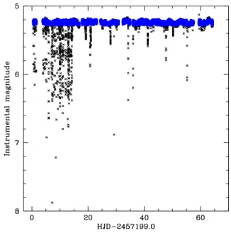
Fig. 1. Removal of outliers from the BRITE photometry of HD 149 404. The black symbols indicate the raw data, the blue symbols stand for the results after MAD filtering and an additional 3 σ clipping around the mean magnitude per spacecraft orbit.
The raw data were extracted with the dedicated pipeline (Popowicz et al. 2017). A periodogram of the raw photometry was computed with the method of Heck et al. (1985) and Gosset et al. (2001) that explicitly accounts for uneven sampling. The strongest peak is found at the orbital frequency (14.827 d−1) of the BRITE-Heweliusz satellite. This is due to extreme outliers appearing in the raw data. Additional cleaning of the data was therefore required.
To remove outliers, we first applied a median absolute de-viation (MAD) filtering, discarding values that deviate by more than
3 × median(|Xi− median(Xi)|), (1)
where Xiis the instrumental magnitude of HD 149 404. In this way, we mostly removed points with very low fluxes. As a sec-ond cleaning step, we then performed a 3 σ clipping around the mean magnitude per spacecraft orbit. This left us with a total of 19 902 data points (see Fig. 1).
The Fourier periodogram of the cleaned time series shows the strongest peak at a frequency of 0.2047 ± 0.0016 d−1 (i.e. a period of 4.885 ± 0.039 day), corresponding within the errors to half the orbital period of HD 149 404 (Porb/2 = 4.9074 ± 0.0004 day, Rauw et al. 2001)2.
2 The full BRITE time series spans∆ t = 63.5 days. The natural width
of the peaks in the periodogram is thus expected to be∆ νnat= 1/∆ t =
1.57 10−2d−1. In our analysis, we conservatively assume that we can
determine the position of a peak in the periodogram with an accuracy of∆ νnat/10.
G. Rauw et al.: BRITE photometry of the massive post-RLOF system HD 149 404
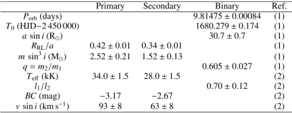
Table 1. Important parameters of HD 149 404
Primary Secondary Binary Ref.
Porb(days) 9.81475 ± 0.00084 (1) T0(HJD−2 450 000) 1680.279 ± 0.174 (1) asin i (R ) 30.7 ± 0.7 (1) RRL/a 0.42 ± 0.01 0.34 ± 0.01 (1) msin3i(M ) 2.52 ± 0.21 1.52 ± 0.13 (1) q= m2/m1 0.605 ± 0.027 (1) Teff(kK) 34.0 ± 1.5 28.0 ± 1.5 (2) l1/l2 0.70 ± 0.12 (2) BC(mag) −3.17 −2.67 (2) vsin i (km s−1) 93 ± 8 63 ± 8 (2)
Notes. RRL, m, and BC are the equivalent radius of the component’s Roche lobe, the mass of the star, and its bolometric correction in the V-band,
respectively. The orbital separation of the system is given by a, and the optical brightness ratio of the primary star to the secondary is l1/l2. The
references are (1) Rauw et al. (2001) and (2) Raucq et al. (2016).
Fig. 2. Top: Full detrended BRITE lightcurve of HD 149 404. All 19 414 data points are shown (red) along with their error bars (black). Bottom: Same, but for the data averaged per spacecraft orbit. This lightcurve contains 708 data points.
As a next step, we pre-whitened our data for the HD 149 404 orbital frequency and twice this frequency by fitting the expres-sion
A1 sin (2 π νorbt+ ψ1)+ A2 sin (4 π νorbt+ ψ2) (2) to the data, where Aj and ψj stand for the semi-amplitude and phase constant of the sine wave of frequency j × νorb. The resid-uals obtained in this way allowed us to check for trends with instrumental parameters such as detector temperature, x and y detector coordinates of the point spread function (PSF) centroid, spacecraft orbital phase, and the PSF smearing parameter. Only weak correlations were found. The strongest correlations con-cerned the detector temperature and x detector coordinates, and they amount to a small fraction (< 15%) of the actual disper-sion of the data. Decorrelation of the photometry with respect to these instrumental parameters was then performed according to the procedure outlined in the BRITE Cookbook 2.0 (Pigul-ski 2018) which is an updated version of the recipe described in Appendix A of Pigulski et al. (2016). In this procedure, we rejected outliers using the Generalized Extreme Studentized De-viate (GESD) algorithm described by Pigulski (2018), indepen-dently of the procedure described above. For this purpose, we
thus started again from the complete original data set (21 448 data points), and first cut off the most extreme values, either in terms of the magnitude or of one of the above instrumental pa-rameters (see Sect. 5.2 in Pigulski 2018). This left us with 20 598 data points. We then rejected the GESD outliers with a level of significance parameter α= 0.05 (see discussion on the choice of this parameter by Pigulski 2018). Next, we removed the space-craft orbits containing fewer than eight data points. A second GESD outlier rejection was performed with α = 0.3 during 1-D decorrelations. As a next step, we removed those spacecraft orbits that have a scatter σ higher than 0.020 mag. We finally performed a third GESD outlier rejection (again with α = 0.3) after 2-D decorrelations, and rejected those spacecraft orbits for which the scatter exceeded 0.017 mag. The full procedure re-sulted in a final set of 19 414 data points. In the following, we focus on these decorrelated data. The typical error bar on the in-dividual decorrelated magnitudes is 0.010 mag. These error bars are computed from the scatter about the decorrelation model for data within each spacecraft orbit (Popowicz et al. 2017). There-fore, all data from a given spacecraft orbit are assigned the same error bar.
2.2. SMEI data
To complement the BRITE data, we also analysed the photome-try coming from the Solar Mass Ejection Imager (SMEI, Jack-son et al. 2004) experiment on board of the Coriolis satellite. Coriolis was in operation between January 2003 and Septem-ber 2012. The SMEI instrument was designed for the imaging of coronal mass ejection (CME) events via the detection of so-lar light scattered by the free electrons in the ejected plasma. For this purpose, the instrument carried three wide field cameras that provided a nearly full sky coverage. To build maps of CME events, the light from background stars had to be subtracted. The sky was covered once per spacecraft revolution leading to a pho-tometric measurement every 101.6 min for each star within the accessible field of view. The PSF was about 1◦. Therefore, nearly eight years of optical photometry of bright stars were collected as a by-product of the SMEI operations3. The SMEI passband was defined by the response of the CCD. The latter reached a maximum quantum efficiency of ≥ 40% in the spectral
re-3 The data processed with the SMEI pipeline (Hick et
al. 2005) are available through the UCSD web page (http://smei.ucsd.edu/new_smei/data&images/stars/timeseries.html).
gion between 6000 and 7500 Å, and dropped below 10 % out-side the spectral range from 4500 to 9500 Å (Eyles et al. 2003). The SMEI passband is thus considerably broader than that of the BRITE-Heweliusz satellite, although they both peak at similar wavelengths.
The time series of SMEI data of HD 149 404 is essentially continuous, except for a gap of about 2.5 months every year due to the location of the star near the ecliptic. The original SMEI photometry contains many outliers and is subject to a number of instrumental variations (see Baade et al. 2018 for a description of these instrumental effects). The most prominent instrumental effect is a modulation by ∼ 0.5 mag with a 1-year period. To cor-rect for this effect, we first phase the raw data with a period of one year. Then, median values are calculated in 200 phase in-tervals. The annual effect is modelled via interpolation between these ‘anchor’ points. We assume that the maximum of the in-terpolated curve indicates the correct flux of the source and add the missing flux to each data point using the interpolated 1-year lightcurve. To remove the outliers in the resulting lightcurve and account for the residual long-term instrumental trends, we apply the following iterative procedure:
• Mean magnitudes over time intervals of a duration T are cal-culated. Following an initial detrending with T = 100 day, we use values of T which are multiples of the binary’s or-bital period, starting from five times the oror-bital period down to one orbital period. This strategy is adopted to avoid alter-ing the orbital signal in the lightcurve.
• The mean magnitudes are interpolated and sigma clipping is used to remove the outliers. We start with a large threshold (5 σ) and make it smaller for the final iterations (3.5 σ). • After a few iterations, the data were detrended for the binary
orbital frequency and its harmonic, and the residuals of this fit were used for further sigma clipping.
The typical error bar on the final detrended SMEI photometry is 0.026 mag.
3. The HD 149 404 lightcurve
The full detrended BRITE lightcurve of HD 149 404 in the red filter is illustrated in the top panel of Fig. 2. Variations with peak-to-peak amplitudes near 0.1 mag are apparent.
3.1. Frequency content of the lightcurve
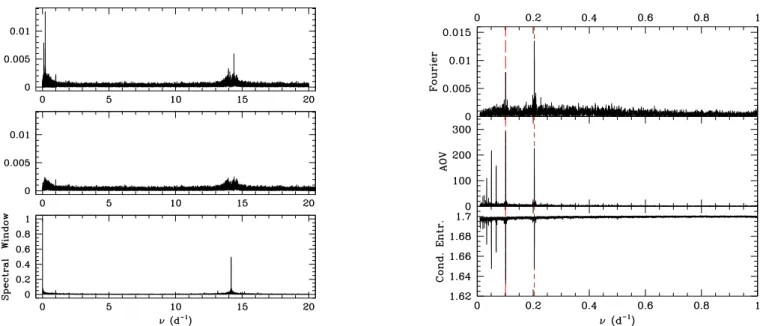
We analysed the decorrelated BRITE-Heweliusz time series of HD 149 404 with a suite of period search algorithms including Fourier periodograms designed for uneven sampling (Heck et al. 1985; Gosset et al. 2001), trial period phase-diagram string length methods (Lafler & Kinman 1965; Renson 1978), trial-period phase-diagram binned analyses of variances (Whittaker & Robinson 1944; Jurkevich 1971; Stellingwerf 1978; Cuypers 1987; Schwarzenberg-Czerny 1989), and conditional entropy (Cincotta 1999; Cincotta et al. 1999; Graham et al. 2013). All these period search methods reveal strong signals at the binary’s orbital period (Porb) and at its second harmonic (Porb/2). As an illustration, the Fourier periodogram, the analysis of vari-ance and the conditional entropy are shown in the right panel of Fig. 3. The entire Fourier power spectrum (top left panel of Fig. 3) is clearly dominated by low frequencies (< 3 d−1). The or-bital frequency of the BRITE-Heweliusz spacecraft (14.827 d−1) introduces a strong aliasing of these frequencies around 15 d−1 (see the spectral window function in the left panel of Fig. 3). The
Fourier periodogram is dominated by a progenitor peak at 2×νorb and a lower one at νorb. This is typical of the alternation of two minima of different depths. The power at the second harmonic frequency is mainly defined by the depth of the minima, whilst the power at the fundamental frequency mainly stems from the differences between the depths of the minima. In the analysis of variance (AoV) periodogram, the peak at the orbital frequency is more important because it is a blend of the genuine peak at νorb, which has a width equal to the natural width∆ νnat, with a narrower subharmonic of 2 × νorb. The presence of peaks at sub-harmonic frequencies is a well-known artefact of phase-diagram methods. Several narrower subharmonic peaks are also visible around 0.05 d−1.
We pre-whitened the decorrelated data for Porband Porb/2 by fitting Eq. 2 to represent the orbital modulation. In this way, we find semi-amplitudes of 0.0067±0.0001 and 0.0139±0.0001 mag for the variations at Porband Porb/2, respectively4.
The Fourier periodograms of the pre-whitened time se-ries (see middle panel of Fig. 3) indicate that any additional, non-orbital, variability in the photometric data occurs at fre-quencies below 3 d−1. There is no outstanding peak in the periodogram after pre-whitening the orbital variations, and for any given frequency the associated semi-amplitude is less than 5 mmag. Moreover, the residual power decreases towards higher frequencies. This situation is reminiscent of the red noise that was found in CoRoT photometry of several O-type stars: HD 46 223 [O4 V((f+))], HD 46 150 [O5.5 V((f))], HD 46 966 [O8 V] (Blomme et al. 2011). Quite recently a similar red noise component was also found in the BRITE photometry of the O4 Ief supergiant ζ Pup (Ramiaramanantsoa et al. 2018). We come back to this aspect in Sect. 3.2. We note that this red noise is not of instrumental origin as it is only rarely seen in BRITE data. For instance, the periodogram of the BRITE data of the β Cep pulsator σ Sco, which was observed in the course of the same campaign as HD 149 404, lacks any increase in the power towards lower frequencies (Pigulski et al. 2018).
The absence of short-period variations implies that, for the study of the orbital variability, we can improve the signal-to-noise ratio of the data by averaging over the duration of the spacecraft orbit (0.06745 day) without any loss of information. We confirmed this by checking that the periodograms of the data averaged over the spacecraft orbit remain essentially identical to those shown in Fig. 3. The typical error bars on the data averaged over the spacecraft orbit is 0.002 mag.
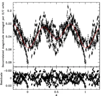
The lightcurve averaged over the duration of the spacecraft orbit contains a total of 708 data points (see the bottom panel of Fig. 2). Figure 4 illustrates this lightcurve as a function of binary orbital phase computed according to the ephemeris of Rauw et al. (2001) where phase 0.0 corresponds to the ON9.7 I secondary star being in inferior conjunction. Ellipsoidal variations with a semi-amplitude near 0.02 mag clearly dominate the lightcurve.
In the pre-whitening process (Eq. 2), we fit the semi-amplitudes A and phase constants ψ of the sine waves corre-sponding to the orbital frequency and its second harmonic si-multaneously for each of these frequencies. Applying the same method to the BRITE data averaged over the spacecraft or-bit, we find that the orbital frequency and its second harmonic have semi-amplitudes of A1 = 0.0070 ± 0.0005 mag and A2 = 0.0135 ± 0.0005 mag, respectively. The resulting best-fit curve
4 The errors on A
jwere determined from the interval of that parameter
that leads to a variation of χχ22n min
by one unit, where n is the number of degrees of freedom.
G. Rauw et al.: BRITE photometry of the massive post-RLOF system HD 149 404
Fig. 3. Left: Fourier periodogram of the decorrelated BRITE photometry of HD 149 404 in the frequency range 0 to 20 d−1(upper panel) and after
pre-whitening of Porband Porb/2 (middle panel). Semi-amplitudes are expressed in magnitudes. The lower panel illustrates the spectral window.
Right: Zoomed-in version of the frequency range between 0 and 1 d−1. The upper, middle, and lower panels illustrate the Fourier periodogram, the
analysis of variance (AoV), and the conditional entropy methods, respectively. In the Fourier and AoV method a detection of a signal corresponds to a peak, whereas in the conditional entropy method a detection is indicated by a minimum. The long- and short-dashed red lines correspond to νorband 2 × νorb, respectively.
Fig. 4. Decorrelated BRITE-Heweliusz photometry of HD 149 404, av-eraged over the spacecraft orbit, folded with the orbital period of the binary system. The red solid curve yields the best-fit Fourier reconstruc-tion consisting of two sine waves: one at the orbital frequency and one at its second harmonic (see Eq. 2). The lower panel illustrates the residuals between the data and this fit.
is illustrated in Fig. 4. There are several important remarks to be made here:
• This best-fit curve obtained through Eq. 2 yields a difference between the depth of the minima near 0.0 and 0.5 of 0.013 mag, and a difference in the maxima at phases 0.25
Fig. 5. Comparison between the BRITE (red open squares) and SMEI (filled blue dots) lightcurve folded with the orbital period of HD 149 404. The data points correspond to normal points built adopt-ing a phase bin of 0.02. To highlight the actual variations, the mean magnitudes are subtracted from both lightcurves.
and 0.75 of 0.005 mag (the maximum at phase 0.75 being brighter). This small difference between the maxima is not significant in view of the non-orbital variability that affects the lightcurve (see Sect. 3.2).
• According to this best fit, there is a slight shift of the phase of primary minimum compared to the ephemeris of Rauw et al. (2001) of 0.02, equivalent to 0.196 days. This shift could result from the uncertainty of Porbaccumulated over the long time interval (5525 days, i.e. 563 orbital cycles) between the
spectroscopic data of Rauw et al. (2001) and the photomet-ric data analysed here, or from the uncertainty of the time of conjunction T0given by Rauw et al. (2001, see Table 1), or from a combination of both effects. Since we cannot disen-tangle these possible causes of the shift, we simply applied a phase shift of 0.02 in our analysis of the lightcurve (Sect. 4). This leads to a revised value of T0 = 2 457 215.9943. An alternative would be a somewhat increased orbital period (9.81510 days, i.e. an adjustment of 0.0036% of Porb). In a binary system with a circular orbit, such as HD 149 404, a difference in depth of the photometric minima could result from several factors. A first possibility would be eclipses of stars of unequal surface temperature. As an alternative, mutual reflec-tion effects between distorted stars of unequal surface brightness will result in ellipsoidal variations with a deeper minimum when the hotter star is in superior conjunction. Finally, the properties of the orbital variations could hint at an asymmetry in the sys-tem. Such an asymmetry could result from a ‘spot’ on the surface of one of the stars (e.g. a bright spot could stem from the impact of the primary stellar wind on the secondary star; see Rauw et al. 2001; Nazé et al. 2002; Thaller et al. 2001).
However, before we accept these asymmetries as true, it is important to understand whether these deviations from a purely symmetrical ellipsoidal modulation are real or result from inter-ference with the remaining frequency content of the lightcurve. For this purpose, we turn to the data collected with the SMEI instrument. Although the SMEI data have much larger error bars than the BRITE data and are subject to possible contamination by neighbouring sources, their large number (21 906 data points after removing the outliers) and their very long time span offer an interesting complement to the BRITE data. To illustrate this point, we compare in Fig. 5 the BRITE and SMEI lightcurves phase-folded over the orbital cycle of HD 149 404 and consist-ing of normal points built by adoptconsist-ing a phase bin of 0.02. Both curves are in very good agreement. The SMEI lightcurve dis-plays slightly lower dispersion, probably because the SMEI data cover more than 200 orbital cycles of HD 149 404 making the normal points less sensitive to the effect of non-orbital variations (see Sect. 3.2).
Appendix A provides detailed information on the peri-odograms built from the SMEI data. The orbital frequency and the second harmonic clearly dominate the periodogram (Figs. A.1 and A.2). For these data, we determine semi-amplitudes of the modulations of A1= 0.0078 ± 0.0002 mag and A2 = 0.0135 ± 0.0002 mag for the orbital period and its second harmonic, respectively. The best-fit two-frequency relation for the SMEI data essentially confirms the conclusions drawn from the BRITE lightcurve with regard to the depth of the minima. In-deed, for the SMEI data, the difference between the depths of the minima at φ = 0.0 and φ = 0.5 amounts to ∼ 0.015 mag. How-ever, the asymmetry between the maxima at quadrature phases appears less pronounced in the SMEI data where the maximum at φ= 0.75 is only ∼ 0.001 mag brighter than that at φ = 0.25.
To get further insight into the origin of the slight di ffer-ences between the BRITE and SMEI lightcurves, we performed a Fourier analysis of the BRITE photometric time series, aver-aged over the duration of the spacecraft orbit, cut into sliding windows of twenty days. The length of the sliding window was chosen to cover at least two full orbital cycles. The resulting time-frequency diagrams are shown in Fig. 6.
From Fig. 6 it appears that the frequency corresponding to Porb/2 is always present, though with an apparently lower semi-amplitude between days 19 and 28. The frequency
correspond-ing to Porb has a more irregular visibility: whilst it is present at the ≥ 6 mmag level most of the time, it gets stronger than 9 mmag between days 22 and 37 (partially overlapping with the episode of reduced strength of the Porb/2 signal) and drops be-low 6 mmag after day 41. It seems thus that both frequencies are present most of the time, but their relevance seems to be affected by the non-orbital variations.
3.2. Non-orbital variability
Within the level of accuracy of the BRITE data, the periodograms of the HD 149 404 photometry reveal no obvious discrete peaks at frequencies other than those corresponding to the orbital mod-ulation. In particular, we note that there are no signals in the range of periods typically associated with β Cep-like pulsations (which span a range from ∼ 0.1 day to ∼ 0.25 day with a me-dian value near 0.17 day, Pigulski & Pojma´nski 2009). Instead, as pointed out above, the frequency content of the non-orbital variations of HD 149 404 is essentially consistent with red noise. In the case of early-type stars, this designation is used for ap-parently stochastic signals whose power increases towards lower frequencies. Several scenarios have been proposed to explain the origin of these variations. They include unresolved randomly ex-cited p-mode oscillations or internal gravity waves generated ei-ther in a subsurface convection zone or directly in the convective core of a massive star (see Ramiaramanantsoa et al. 2018, and references therein).
Though the power of the red noise is spread out over a range of frequencies, the residuals seen in Fig. 4 indicate that it can produce variations with peak-to-peak amplitudes up to 40 mmag. This is larger than the 20 mmag peak-to-peak amplitude reported by Ramiaramanantsoa et al. (2018) in the case of ζ Pup.
We model the non-orbital variations following the approach of Blomme et al. (2011) and Uuh-Sonda et al. (2014), which is based on the formalism of Stanishev et al. (2002). We thus fit the expression
A(ν)= A0
1+ (2 π τ ν)γ (3)
to the periodogram (see Fig. 7). Here A(ν) is the semi-amplitude derived from the Fourier periodogram, A0 is a scaling factor, γ is the slope of the linear part (in a log-log plot), and τ (in days) is an indication of the mean duration of the dominant features in the lightcurve. We perform the fit up to a frequency of 4.0 d−1. At higher frequencies, up to 7.414 d−1 (i.e. up to the Nyquist frequency of the spacecraft orbit), the periodogram is essentially consistent with white noise.
Our best-fit γ value (1.93 ± 0.11) is between the values (0.91 – 0.96) of the three early-type stars investigated by Blomme et al. (2011) and the value (2.3) obtained for Plaskett’s Star by Mahy et al. (2011). The τ value (0.138 ± 0.005 day) also falls in the range observed for these stars (0.08 – 0.17 day, Blomme et al. 2011; Mahy et al. 2011).
To assess the impact of the intrinsic variations on the orbital modulation, and more specifically to understand whether these intrinsic variations can explain the slight differences between the BRITE and SMEI lightcurves, we generated 10 000 synthetic BRITElightcurves using a Monte Carlo simulator. We assume that the orbital signal consists of the best-fit two frequency de-composition of the SMEI lightcurve and a red noise component simulated using the recipe of Timmer & König (1995) with the A(ν) formalism described in Eq. 3 above. We adopt the same sampling as for the spacecraft-orbit averaged BRITE lightcurve.
G. Rauw et al.: BRITE photometry of the massive post-RLOF system HD 149 404
Fig. 6. Time-frequency diagrams of the decorrelated photometry of HD 149 404, averaged over the spacecraft orbit before (upper panels) and after (lower panels) pre-whitening for Porband Porb/2. The left panels illustrate the evolution of the Fourier periodogram as a function of the heliocentric
Julian day at the middle of the 20-day sliding window (see text). Dark blue, light blue, and cyan stand respectively for semi-amplitudes ≥ 9 mmag, ≥ 6 mmag, and ≥ 3 mmag. The right panels yield the Fourier periodograms over the full duration of the BRITE campaign.
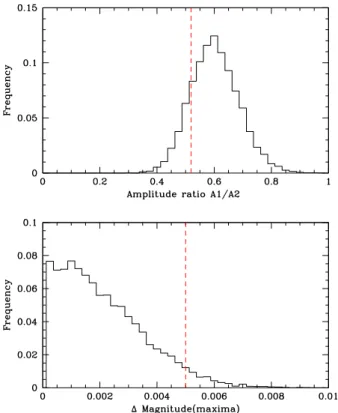
We then fit an expression equivalent to Eq. 2 to each synthetic lightcurve. The results are illustrated by the two histograms in Fig. 8. The top panel displays the ratio between the semi-amplitudes of the sine waves corresponding to the orbital period (A1) and its second harmonic (A2). As can be seen, the distribu-tion of the A1-to-A2 ratios for the simulated data peaks near the value determined for the SMEI data, (A1/A2)SMEI= 0.58, which we used as input in our simulations. The value determined from the BRITE data, (A1/A2)BRITE = 0.52 ± 0.05, is very close to the peak of the distribution of the simulated data and is thus not exceptional given the properties of the red noise.
The bottom panel of Fig. 8 illustrates the difference in mag-nitude between the two maxima of the simulated lightcurves. Among the 10 000 synthetic lightcurves, 568 yield a difference between the maxima that is equal to or larger than the observed value. We thus conclude that, in view of the non-orbital vari-ations, the significance level of the observed difference of the
maxima is about 5.7%. The slight asymmetry of the BRITE lightcurve around the maxima is thus likely insignificant.
From these simulations, we conclude that the red noise ponent can affect the apparent asymmetry of the orbital com-ponent of the lightcurve of HD 149 404 and can thus explain the slight differences between the fits of the BRITE and SMEI lightcurves. In Sect. 4, we consider various options to extract and model the orbital part of the lightcurve.
4. Modelling the orbital variations
In view of the above discussion about possible asymmetries in the orbital lightcurve, we considered several approaches to fit the orbital part of the photometric variations of HD 149 404. We first focused on the decorrelated BRITE photometry averaged over the spacecraft orbit (option I). Then we analysed the lightcurves consisting of normal points built by adopting phase bins of 0.02
0.001 0.01 0.1 1 0.0001 0.0005 0.001 0.005 0.01
Fig. 7. Log-log plot of the semi-amplitude spectrum of the decorrelated photometry, averaged over the spacecraft orbit. The semi-amplitude spectrum is shown out to the Nyquist frequency of the spacecraft orbit (7.414 d−1). The red line corresponds to the best-fit red-noise relation
with A0 = 0.0021, γ = 1.93 ± 0.11 and τ = 0.138 ± 0.005 day, fit up to
a frequency of 4.0 d−1.
Fig. 8. Top: Histogram of the ratio between the semi-amplitudes of the orbital frequency and its second harmonic as obtained with the Monte Carlo simulations. The dashed vertical line indicates the observed value of the semi-amplitude ratio obtained via pre-whitening of the lightcurve averaged over the BRITE spacecraft orbit (A1/A2)BRITE = 0.52 ± 0.05.
Bottom: Histogram of the difference between the two maxima of the simulated lightcurves. The observed value of this difference in the BRITElightcurve (' 0.005 mag) is again shown by the dashed verti-cal line.
(option II and III for the BRITE and SMEI lightcurves, respec-tively).
We analysed the lightcurve with the eclipsing binary star code nightfall (version 1.86) developed by R. Wichmann, M. Kuster and P. Risse5. This code uses the Roche potential to
de-5 The code is available at the URL: http:
//www.hs.uni-hamburg.de/DE/Ins/Per/Wichmann/Nightfall.html
scribe the shape of the stars, and for the simplest cases (two stars on a circular orbit with no stellar spots or disks), six parame-ters are required to describe the system: the mass-ratio, the or-bital inclination, the primary and secondary filling factors (de-fined as the ratio of the stellar polar radius to the polar radius of the associated Roche lobe), and the primary and secondary fective temperatures. We fixed the mass-ratio and the stellar ef-fective temperatures to the values obtained in the spectroscopic analyses of Rauw et al. (2001) and Raucq et al. (2016) listed in Table 1. We further adopted a quadratic limb-darkening law us-ing limb-darkenus-ing coefficients from Claret (2000). Reflection effects were accounted for by considering the mutual irradia-tion of all pairs of surface elements of the two stars (Hendry & Mochnacki 1992). To approximate the non-standard passbands of the BRITE and SMEI instruments in the nightfall calcula-tions, we used the Johnson-V passband as a proxy. Whilst this is clearly an approximation, it should not impact our conclusions as both components of HD 149 404 are relatively close in spec-tral type and thus have specspec-tral energy distributions in the optical that are quite similar. Finally, since we are analysing broadband photometry in a single passband, we used the black-body law to compute the relative contribution from each star to the total light. The spectroscopic optical brightness ratio of the system (see Table 1) can be converted into a bolometric luminosity ratio of Lbol,1/Lbol,2 = 1.11 ± 0.19 adopting the bolometric correc-tions inferred by Raucq et al. (2016). Then, knowing the effec-tive temperatures, we obtain the ratio between the stellar radii (R1/R2= 0.713 ± 0.116) and hence between the Roche lobe fill-ing factors: f1/ f2= 0.566 ± 0.093.
4.1. Models without spots
As a first step, we left the primary and secondary Roche lobe fill-ing factors and the orbital inclination unconstrained in the fittfill-ing procedure. The best fits obtained in this way yield primary filling factors that are close to, or even larger than, the secondary filling factor. These solutions are thus significantly at odds with the ra-tio of the filling factors inferred from the spectroscopic analysis ( f1/ f2= 0.566 ± 0.093, see above).
To search for solutions that are consistent with the spectro-scopic ratio of stellar radii, we thus constrained the values of the filling factors according to the considerations above. For this purpose, we scanned the parameter space in a systematic way. For each value of f2 between 0.60 and 1.00 (in steps of 0.02), we tested three values of f1, corresponding respectively to ratios f1/ f2−σf1/ f2, f1/ f2, and f1/ f2+ σf1/ f2. With these combinations
of filling factors fixed in the fitting procedure, the only remain-ing fittremain-ing parameter is the orbital inclination. We thus ran the nightfall code to search for the orbital inclination that yields the best-quality fit. As a first step, we included the detailed treat-ment of the mutual reflection between the stars, but omitted any spots on the stars.
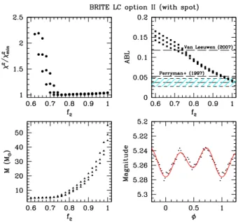
The results are illustrated in Fig. 9 for the three options of the lightcurve defined above. For each option, Fig. 9 provides the χ2/χ2
min, the astrometry-based luminosity (Arenou & Luri 1999)
ABL= 100.2 MV, (4)
where MV is the absolute magnitude of the system inferred from the lightcurve solution, the total mass of the binary, and a com-parison between the best-fit solution that has an ABL in agree-ment with the Gaia-DR2 parallax (see below) and the lightcurve. There are several results that are worth noting here. First of all, the larger the secondary filling factor, the lower the
or-G. Rauw et al.: BRITE photometry of the massive post-RLOF system HD 149 404
Fig. 9. Properties of the best-fit models (assuming no sur-face spots) of the lightcurves for option I (spacecraft-orbit-averaged BRITE photometry, upper left quadrant), option II (binned BRITE lightcurve, upper right quadrant), and option III (binned SMEI lightcurve, lower left quadrant). For each option, the panels illustrate the fit quality, the astrometry-based lumi-nosity ABL (see text), and the total mass of the system as a function of the secondary filling factor. The blue hatched area in the ABL panels indicates the value of ABLDR2and its associated
uncertainty. The lower right panel of each quadrant compares the lightcurve with the fit with the lowest χ2 that also agrees
with the value of ABLDR2(see Table 2).
bital inclination required to reproduce the observed lightcurves (see Fig. 10). For f2 = 1.00, we find the lowest values of i which range between 23 and 26◦, depending on the option of the lightcurve. Values of f2≤ 0.70 are generally associated with i ≥67◦and the corresponding synthetic lightcurves display graz-ing eclipses or even eclipses for the lowest values of f2. Except for the BRITE lightcurve built from the normal points (option II), the presence of these (grazing) eclipses leads to a rapid degrada-tion of the fit quality. In general, the values of the χ2of the fits are far from what is expected for a statistically good fit6. For lightcurve option I and probably also option II, this situation re-flects the presence of the strong red noise component on top of the ellipsoidal variations (see Sect. 3.2). In Sect. 4.2, we investi-gate how the fit quality changes when we include a spot on the secondary surface. Meanwhile, we note that it is generally di ffi-cult to identify an overall best-fit solution of the lightcurve based on the behaviour of the χ2value alone.
Additional constraints can be obtained from the dependence of the absolute magnitude on f2. Indeed, once we have ob-tained a full solution of the lightcurve, we can combine the
6 These values are nevertheless very close to those found for the best
solutions with f1and f2left unconstrained. Hence, constraining the ratio
f1/ f2does not impact the fit quality too much.
Roche lobe filling factors with the orbital solution of Rauw et al. (2001) and the bolometric corrections and effective tempera-tures of Raucq et al. (2016) to compute the absolute magnitude of the HD 149 404 binary system (see the parameters in Table 1). This absolute magnitude strongly varies as a function of f2, and can thus be compared to the absolute magnitude based on the apparent magnitude and a distance estimate. For this purpose, we use the apparent magnitude mV = 5.48 ± 0.02 and colour-index B − V = 0.39 ± 0.02 (Reed 2005). We further adopt the intrinsic colour (B − V)0 = −0.26 (Martins & Plez 2006) and assume RV = 3.1. Using the Hipparcos data, Perryman et al. (1997) quoted a parallax of $= 1.07 ± 0.89 milliarcsec, whilst the revised reduction of the Hipparcos data led to a parallax of $ = 2.40 ± 0.36 milliarcsec (Van Leeuwen 2007). A signifi-cantly larger distance (1753 ± 293 pc, corresponding to $ = 0.57 ± 0.10 milliarcsec) was estimated by Megier et al. (2009) based on the strength of the interstellar Ca ii H and K lines. Most recently, the second Gaia data release (DR2, Gaia Collaboration 2018) quoted a parallax of $= 0.760 ± 0.165 milliarcsec. This value overlaps within the errors with the original Hipparcos par-allax and the estimate of Megier et al. (2009), but rules out the value from the revised Hipparcos reduction. Whilst the DR2 cer-tainly provides the most accurate determination of the parallax of
Fig. 10. Secondary filling factor f2 as a function of orbital inclination
for the best-fit lightcurve models of option II (binned BRITE lightcurve) without a spot on the secondary (filled dots) and including a spot (red open diamonds). For each value of f2three models are shown,
corre-sponding to the three values of f1investigated.
HD 149 404 to date, we need to be careful when comparing our results with the DR2. Luri et al. (2018) pointed out that a Gaus-sian probability density function (PDF) of the measured paral-lax $ results in a non-Gaussian PDF for the distance estimator d= 1/$. Even worse, the shape of the PDF of d depends on the unknown value of the true parallax $true. As a way to avoid this problem, Luri et al. (2018) suggest expressing the quantity to be measured directly in the space of parallaxes. In our case, this can be done using the astrometry-based luminosity ABL (Arenou & Luri 1999). According to Eq. 4, it follows that
ABL= 100.2 MV = $ 100.2 (mV−AV+5) (5)
For HD 149 404, the DR2 parallax results in ABLDR2= (3.74 ± 0.98) 10−2. This value and its associated error are shown by the hatched area in the plots of Fig. 9. In a recent study, Stassun & Torres (2018) compared the Gaia-DR2 parallaxes of 89 eclips-ing binaries against the distances derived from analyses of the lightcurves. Stassun & Torres (2018) found evidence for a sys-tematic offset by 0.082 ± 0.033 milliarcsec with the Gaia-DR2 parallaxes being too small. Accounting for such a systematic shift, does not affect our conclusion regarding the value of f2: only solutions with f2≥ 0.96 agree with the ABLDR2value.
Table 2. Parameters of the best fit with a simple binary model consistent with ABLDR2
LC option f1 f2 i(◦) χ2
I 0.646 0.980 28.8 28.6
II 0.659 1.000 29.2 58.3
III 0.646 0.980 30.4 4.4
Notes. The models account for mutual reflection, but do not include any spots. The corresponding fits are illustrated in Fig. 9. The last column quotes the normalized χ2of the fit. For comparison, the χ2
minvalues for
the full parameter space that we explored are 28.6, 54.2, and 4.0 for lightcurve options I, II, and III, respectively.
4.2. Models with spots
We also test models with a spot on the surface of the secondary. We chose to put the spot on the secondary star because the anal-yses of the emission line profile variations of Rauw et al. (2001), Nazé et al. (2002), and Thaller et al. (2001) suggest that the wind of the primary dominates over that of the secondary, possibly leading to a crash of the primary wind onto the surface of the secondary. The spot is assumed to be located on the secondary’s equator, but we leave its size and longitude as free parameters. The spot can be either brighter or fainter than the surrounding stellar surface. In this way, we now have for each combination of f1 and f2, a total of four free parameters: the orbital incli-nation i, plus the longitude, radius, and dim-factor7of the spot. From the point of view of the fit quality, there is obviously some degeneracy between a dim-factor larger or less than 1.0 and the longitude of the spot. Finally, we note that there is a degeneracy between the size of the spot and the dim-factor: to the first or-der, bigger spots with dim-factors closer to unity yield the same effect on the lightcurve as smaller spots with dim-factors that deviate more from unity.
As a result of the degeneracies discussed above, the spot pa-rameters inferred from the fits are certainly not unique. Nev-ertheless, including such a spot substantially improves the fit quality (see Fig. 11 and Table 3). The only exception is option I, where the improvement is marginal because the high value of the χ2 in this case mostly reflects the impact of the red noise component.
In addition to the general trends for the fits discussed in Sect. 4.1, Fig. 11 reveals that the χ2 displays an even flatter be-haviour between f2 = 0.72 and f2 = 1.00 than in Fig. 9. This observation clearly emphasizes the need for additional indepen-dent constraints (provided by the Gaia-DR2 parallax) to over-come this degeneracy.
Whether we consider the models with or without a spot on the secondary’s surface, we reach the same general conclusions for each of the three lightcurve options: in order for the model parameters to agree with the Gaia-DR2 parallax, we need a secondary filling factor f2 ≥ 0.96 along with an orbital inclination i in the range between 23◦and 31◦.
5. Discussion
5.1. Brightness ratio
A puzzling problem that affects the analysis of several evolved massive binaries is the discrepancy between the visual bright-ness ratio inferred from spectroscopic and photometric analyses. For instance, in the case of LSS 3074, Raucq et al. (2017) found a spectroscopic brightness ratio between the primary and sec-ondary close to 2.5, whilst the photometric data favoured a value near 1.1. Raucq et al. (2017) tentatively attributed this effect to the impact of strong radiation pressure on the shape of the bi-nary components (see e.g. Fig. 3 in Palate et al. 2013). A very similar discrepancy was reported by Linder (2008) in the case of 29 CMa.
At first sight, this discrepancy is also present in the case of HD 149 404. As pointed out above, leaving the Roche lobe filling factors unconstrained in the fits of the orbital part of the lightcurve actually leads to situations where both stars have
7 The dim-factor is defined as the ratio of the effective temperature of
the spot region to the effective temperature of the surrounding stellar surface.
G. Rauw et al.: BRITE photometry of the massive post-RLOF system HD 149 404
Fig. 11. Same as Fig. 9, but for the fits including a spot on the secondary surface.
Table 3. Parameters of the best fit with a binary model including a spotted secondary and consistent with ABLDR2
LC option f1 f2 i(◦) Spot χ2
long. (◦) radius (◦) dim
I 0.646 0.980 28.4 95.6 7.6 0.65 28.3
II 0.464 0.980 27.0 212.9 22.9 1.12 27.9
III 0.646 0.980 29.2 203.4 51.9 1.03 1.6
Notes. The corresponding fits are illustrated in Fig. 11. For comparison, the χ2
minvalues for the full parameter space that we explored are 28.1,
27.1, and 1.5 for lightcurve options I, II, and III, respectively. Spot longitudes of 90◦
and 270◦
correspond to the trailing and leading side of the secondary star, respectively.
nearly identical filling factors. Given the mass-ratio and the ef-fective temperatures of the stars, these configurations would cor-respond to bolometric flux ratios lbol,1/lbol,2 ' 3.3, which in turn implies an optical brightness ratio l1/l2 ' 2.1, significantly at odds with the spectroscopic value of 0.70 ± 0.12. To check whether or not a visual brightness ratio of 2.1 could be consistent with the spectroscopic data, we performed test calculations with the CMFGEN code to fit the reconstructed spectra of the two components assuming l1/l2 = 2.1. We could not achieve a good fit of the strength of the spectral lines in the reconstructed spec-tra. Moreover, this brightness ratio would also affect the log g
of the primary star, which would change from 3.55 to 3.10 (er-ror of 0.15 dex, Raucq et al. 2016), leading to further difficulties in reproducing the reconstructed spectra. We thus favoured the solutions of the lightcurve where the filling factors were con-strained to be consistent with l1/l2 = 0.70 ± 0.12. In our case, the difference in the quality of the fits between constrained and unconstrained values of the filling factors is relatively small. We thus conclude, at least in the case of HD 149 404, that the photo-metric lightcurve is consistent with the spectroscopic brightness ratio.
5.2. Stellar parameters
The fits of the BRITE lightcurve combined with independent in-formation from the Gaia-DR2 lead to inclinations in the range between 23◦and 31◦. The confidence range on i, however, is not centred on that of the Gaia parallax. The lower the inclination i, the closer the ABL parameter is to the value corresponding to the Gaia parallax. While values of i below 23◦ would be al-lowed by the ABL parameter, they are excluded by the fact that f2should not exceed unity (a contact or overcontact configura-tion is ruled out by the spectroscopic brightness ratio and by the shape of the lightcurve). Therefore, whilst it appears likely that the actual value of i is closer to 23◦ than to 31◦, the currently available information does not allow us to formulate more strin-gent constraints on this parameter.
The remaining uncertainty on i has important consequences on our knowledge of the stellar masses. For i = 23◦, we obtain m1 = (42.2 ± 3.5) M and m2 = (25.5 ± 2.2) M , whilst i= 31◦ instead leads to m1 = (18.4 ± 1.5) M and m2= (11.1 ± 1.0) M . Rauw et al. (2001) inferred an inclination of 21◦ by compar-ing the minimum dynamical masses of the stars with typical masses of stars of the same spectral type as quoted by Howarth & Prinja (1989). However, this comparison could be biased. On the one hand, we now know that the present-day secondary star has undergone a Roche lobe overflow episode in the past (as the mass donor) and displays non-solar surface abundances (Raucq et al. 2016). The mass-luminosity relation of this star could thus strongly deviate from that of genuine O-stars. A sim-ilar but less extreme deviation could apply to the primary star (the mass gainer). On the other hand, the typical masses of O-type stars were revised by Martins et al. (2005). Therefore, if we instead compare the primary minimum mass with the spectro-scopic mass of an O7.5 I star as quoted by Martins et al. (2005), we find that an inclination of (24.3 ± 0.7)◦ is required for the primary to have a typical mass for its spectral type.
In summary, whilst we cannot rule out the possibility that the components of HD 149 404 might be overluminous for their masses, we find that by assembling all the currently available information, it seems likely that at least the mass of the primary is relatively close to typical, unlike the situation encountered in the post-RLOF contact binary LSS 3074 (Raucq et al. 2017).
For each lightcurve solution that falls into the acceptable range of ABL values, we compute the associated log g values of both stars. In this way, we obtain log g1 = 3.45 ± 0.14 and log g2= 2.94±0.03, which are in good agreement with the spec-troscopic values of log g1= 3.55 ± 0.15 and log g2= 3.05 ± 0.15 (Raucq et al. 2016). The same models have log L1/L = 5.47 ± 0.10 and log L2/L = 5.42 ± 0.08. We can visualize these results in the Hertzsprung-Russell diagram (HRD) and the log g–log Teff diagram (see Fig. 12). For qualitative comparison, we also show the evolutionary tracks of Ekström et al. (2012) with an initial rotational velocity of 0.4 × vcrit and of Brott et al. (2011) with initial rotational velocities that are closest to the v sin i values determined by Raucq et al. (2016) and corrected for i in the range between 23◦and 31◦. In addition to different assumptions on the solar metallicity and the evolution of angular momen-tum, these models also differ in terms of the adopted core over-shooting parameter: 0.1 for Ekström et al. (2012) and 0.335 for Brott et al. (2011). Such single-star evolutionary models are cer-tainly not representative of the evolution of the components of HD 149 404, especially for the present-day secondary which has undergone a RLOF episode; nonetheless, they can provide some interesting information.
For the primary, the position in the HRD falls between single-star evolutionary tracks of 30 – 40 M , in relatively good agreement with the mass estimates that we have obtained above. This result is supported by the position of the star in the log g– log Teffdiagram. All in all, the properties of this star seem in fair agreement with the expected value given its current mass. This conclusion is consistent with a scenario where the mass gainer was not totally mixed during the RLOF episode and thus rapidly settled onto an evolutionary track corresponding to its new mass (Vanbeveren et al. 1998).
The situation of the secondary is more complex. In the HRD its position suggests a mass between 25 and 30 M for the Ek-ström et al. (2012) tracks or between 30 and 35 M for the Brott et al. (2011) models. Not surprisingly, in view of its evolutionary state, the secondary thus appears overluminous for its mass. The secondary is also far away from the tracks corresponding to its mass in the log g–log Teffdiagram.
Assuming that the rotational axes of the stars are aligned with their orbital axis, we use the v sin i values determined by Raucq et al. (2016) along with the radii determined for the light curve solutions that fall into the acceptable range of ABL val-ues to assess the rotation rates of both stars. In this way, we find Prot,1 = (3.98 ± 0.52) days and Prot,2 = (8.13 ± 0.13) days. Our results thus confirm the strong asynchronicity of the rotation of the primary star noted by Raucq et al. (2016). This supports the idea that the primary was spun up during the mass and angu-lar momentum transfer. The above rotation periods correspond to roughly 36% of the critical rotation rates for both stars. This result, along with our discussion of the primary position in the HRD, suggests that the primary was not fully mixed during the mass transfer as it would otherwise display an even faster ro-tation. It might also imply that mass transfer was more conser-vative than suggested by the models of Petrovic et al. (2005). Finally, we note that the rotation of the secondary is faster than the orbital rate. This situation can be explained if the binary or-bital period increased as a result of the RLOF mass exchange as predicted by Vanbeveren et al. (1998).
5.3. Wind–wind and binary interactions
As shown in Sect. 4, including a spot on the surface of the sec-ondary improves the fits of the orbital lightcurve of HD 149 404. This spot asymmetry could also affect the strength of the spec-tral lines. Previous studies have noted variations in the equivalent widths (EWs) of the primary and secondary absorption lines with orbital phase (Stickland & Koch 1996; Nazé et al. 2002; Rauw et al. 2001), which were considered manifestations of the so-called Struve-Sahade effect. In the case of HD 149 404 these variations concern both the primary and secondary star, which vary in op-posite ways. For instance, the equivalent width of the He i λ 4471 line is larger at phase 0.25 than at phase 0.75 for the primary, whilst the reverse situation is seen for the secondary (Nazé et al. 2002). In Rauw et al. (2001), we considered the possibility that the variations in the equivalent widths could reflect variations in the continuum at the level of a few percent. Given the amplitude of the variations of the EWs (a factor of two for the He i λ 4471 line, Nazé et al. 2002), this scenario was deemed unlikely, and we instead favoured the possibility of blends with weak emis-sion wings. The results obtained in the present study confirm that the variations in the continuum are indeed rather modest, but they also highlight an aspect which was not considered in the previous work: the spotted region is not only brighter, but also hotter than the neighbouring parts of the stellar surface. For temperature-sensitive spectral lines, the amplitude of the change
G. Rauw et al.: BRITE photometry of the massive post-RLOF system HD 149 404
Fig. 12. Position of the components of HD 149 404 in the Hertzsprung-Russell diagram (upper panels) and in the log g – log Teffdiagram (lower
panels). The filled (resp. empty) symbols correspond to the primary (resp. secondary) star. In the left panels, evolutionary tracks for single massive stars at solar metallicity and initially rotating at 0.4 × vcritfrom Ekström et al. (2012) are overplotted. The dashed red lines correspond to isochrones
of 5.0 and 7.9 Myr. In the right panels we show evolutionary tracks from Brott et al. (2011). The solid lines yield tracks with initial equatorial rotational velocities near 100 km s−1(112, 111, 110, 109, and 109 km s−1 for the 15, 20, 25, 30, and 35 M
models), whilst the dashed tracks
correspond to initial equatorial rotational velocities near 200 km s−1(216, 214, and 213 km s−1for the 35, 40, and 50 M
models).
in EW can exceed the change in the level of the continuum by a significant factor.
In Sect. 4.2, we argue that the spot is likely related to the in-teraction between the stellar winds of HD 149 404. An alterna-tive could be a spot induced by a strong magnetic activity. How-ever, unless this feature comes from a localized magnetic field, this is rather unlikely to be the case here. Indeed, dedicated spec-tropolarimetric observations resulted in no detection of a global large-scale magnetic field associated with either the primary or the secondary star (Nazé et al. 2017). Therefore, interactions be-tween the stars and their wind interaction zone are more likely to be responsible for the spot. Since we show here that the sec-ondary is close to filling its Roche lobe, it seems rather unlikely that its stellar wind can reach a high speed before it collides with the primary’s wind. Given the short orbital period, the ratio of vorbto vwindmust be rather large and the wind interaction zone
in HD 149 404 must therefore be strongly bent by the Coriolis pseudoforces. This situation brings the strongly distorted inter-action region very close to the secondary’s surface on the leading side of the star and could thus lead to a strong local heating ef-fect.
An alternative explanation for the spot could be an ongoing Roche lobe overflow of the secondary. In such a configuration, the gas stream flowing through the first Lagrangian point L1 is expected to impact the primary star on its rear side (Lubow & Shu 1975), thereby leading to a hot spot on the rear of the mary (which is most visible around phases 0.75 when the pri-mary is receding from the observer). In Sect. 4.2 we assume the spot to be located on the surface of the secondary star. However, there is a degeneracy between a spot on the leading side of one star and a similar spot on the rear side of its companion. This ongoing RLOF scenario would explain the changes of the
ap-parent spectral type of the primary from O6.5 near φ = 0.75 to O7.5 around φ = 0.25 as reported by Nazé et al. (2002). Whilst we cannot discard this possibility with the currently available data, we do note that this scenario only works for a subfamily of the models considered here. The ongoing RLOF, and thus the hot spot on the primary star, only exist for a semi-detached con-figuration with the secondary exactly filling its Roche lobe (i.e.
f2= 1.0).
6. Summary and conclusions
The BRITE-Heweliusz lightcurve and archival SMEI data of HD 149 404 reveal two types of photometric variability: a deter-ministic modulation with the orbital period and a stochastic sig-nal consistent with red noise. The present study mainly focused on the orbital component, which we interpreted as ellipsoidal variations. These variations could be equally well explained by models covering a wide range of values of the filling factors and orbital inclination. However, combining the constraints from the BRITE and SMEI data with the Gaia-DR2 parallax, we were able to constrain the secondary filling factor to f2 ≥ 0.96 and the orbital inclination to 23◦ ≤ i ≤ 31◦. These constraints lead to a clearer view of the properties of the system and allow us to confirm and refine some of the previous assertions regarding the post-RLOF status of this binary. HD 149 404 should now be considered as a test case for theoretical binary evolution models: whilst many of its properties qualitatively agree with the expec-tations for post-RLOF systems, some quantitative aspects prob-ably require further theoretical modelling.
Acknowledgements. The operation of BRITE-Heweliusz is supported by a SPUB grant of the Polish Ministry of Science and Higher Education (MNiSW). This work has made use of results from the ESA space mission Gaia, the data from which were processed by the Gaia Data Processing and Analysis Consortium. The Liège team acknowledges financial support through an ARC grant for Con-certed Research Actions, financed by the Federation Wallonia-Brussels, from the Fonds de la Recherche Scientifique (FRS/FNRS) through an FRS/FNRS Re-search Project (T.0100.15), and through two PRODEX contracts (Belspo) re-lated to XMM-Newton and Gaia DPAC. GH acknowledges support from the Polish NCN grant 2015/18/A/ST9/00578. APi acknowledges support from the NCN grant 2016/21/B/ST9/01126. AFJM is grateful for financial aid from NSERC (Canada) and FQRNT (Québec). APo was supported by NCN grant 2016/21/D/ST9/0065. SMR and GAW acknowledge support from the NSERC (Canada). KZ acknowledges support from the Austrian Space Application Pro-gramme (ASAP) of the Austrian Research Promotion Agency (FFG).
G. Rauw et al.: BRITE photometry of the massive post-RLOF system HD 149 404
Appendix A: Fourier periodogram of the SMEI data
Figures A.1 and A.2 illustrate the Fourier periodogram of the SMEI time series of HD 149 404. The entire SMEI data set covers 2448 days, leading to a natural width of the peaks of 3.51 10−4d−1. In Fig. A.1, we consider the SMEI time series after correcting for the annual modulation and other long-term trends and removal of clear outliers. The strongest peaks are at frequen-cies of (0.203786±0.000035) d−1and (0.101912±0.000035) d−1, corresponding respectively to periods of (4.90711±0.00085) and (9.81239 ± 0.00338) days. These values agree within the error bars with half the orbital period and the orbital period as deter-mined from radial velocities (see Rauw et al. 2001, and Table 1). The periodogram further displays some peaks near integer multi-ples of 1 d−1. These features are of instrumental origin. We also note a peak at 0.227 d−1 which could be of astrophysical ori-gin. Given the coarse PSF of the SMEI instrument, we cannot exclude the possibility that this signal arises in another object, unrelated to HD 149 404. The SIMBAD catalogue lists 145 ob-jects within a radius of 400 around HD 149 404. The majority of these sources are fainter than 9th magnitude and should thus not affect the SMEI photometry in a significant way. There are, however, three exceptions: V 1061 Sco (M1, V = 8.26) at 15.20, HD 149 340 (A0 IV, V = 7.81) at 21.90, and HD 149 711 (≡ V 1003 Sco, B2 V, V= 5.83) at 39.50. V 1061 Sco is classified as a long-period variable and is therefore unlikely to be responsible for the 0.227 d−1peak. No information is available about vari-ability of HD 149 340. HD 149 711 is classified as an ellipsoidal variable, though no period of variability is available in the litera-ture. The International Variable Star Index (VSX) catalogue does not list any known variable star with a period corresponding to the 0.227 d−1frequency in the vicinity of HD 149 404.
In Fig. A.2, we provide the periodograms after removing the signals at the 1 d−1 (four peaks near that frequency) and 2 d−1 (a single peak) frequencies. Except for a small shift of the peak corresponding to the orbital period, the strongest peaks have the same frequencies as in Fig. A.1: (0.203786 ± 0.000035) d−1and (0.101911 ± 0.000035) d−1, corresponding respectively to peri-ods of (4.90711 ± 0.00085) and (9.81248 ± 0.00338) days. All these conclusions are backed up by the other period search meth-ods (see the right panels of Figs. A.1 and A.2). Using our pre-whitening routine with the frequencies corresponding to Porb(as quoted in Table 1) and its second harmonic, we determine semi-amplitudes of the modulations of A1= 0.0078 ± 0.0002 mag and A2= 0.0135 ± 0.0002 mag.
The periodograms of the SMEI data also display a red noise component. At first sight this looks similar to the red noise seen in the BRITE data; however, we note that SMEI data are affected by a red noise of instrumental origin and it is not possible to quantify the relative importance of the two contributions to the red noise seen in this periodogram.
References
Arenou, F., & Luri, X. 1999, in Harmonizing Cosmic Distance Scales in a Post-HIPPARCOS Era, eds. D. Egret & A. Heck, ASPC, 167, 13
Baade, D., Pigulski, A., Rivinius, T., et al. 2018, A&A, 610, A70 Blomme, R., Mahy, L., Catala, C., et al. 2011, A&A, 533, A4 Brott, I., de Mink, S.E., Cantiello, M., et al. 2011, A&A, 530, A115 Cincotta, P.M. 1999, MNRAS, 307, 941
Cincotta, P.M., Helmi, A., Mendez, M., Nunez, J.A., & Vucetich, H. 1999, MN-RAS, 302, 582
Claret, A. 2000, A&A, 363, 1081
Cuypers, J. 1987, Mededelingen van de Koninklijke academie voor Wetenschap-pen, Letteren en Schone Kunsten van België, Academiae Analecta, Jaargang 49, Nr 3
Ekström, S., Georgy, C., Eggenberger, P., et al. 2012, A&A, 537, A146
Eyles, C.J., Simnett, G.M., Cooke, M.P., et al. 2003, Solar Phys., 217, 319 Gaia Collaboration, Brown, A.G.A, Vallenari, A., Prusti, T., de Bruijne, J.H.J.,
Babusiaux, C., & Bailer-Jones, C.A.L. 2018, A&A, 616, A1
Gosset, E., Royer, P., Rauw, G., Manfroid, J., & Vreux, J.-M. 2001, MNRAS, 327, 435
Graham, M.J., Drake, A.J., Djorgovski, S.G., Mahabal, A.A., & Donalek, C. 2013, MNRAS, 434, 2629
Heck, A., Manfroid, J., & Mersch, G. 1985, A&AS, 59, 63 Hendry, P.D., & Mochnacki, S.W. 1992, ApJ, 399, 603
Hick, P.P., Buffington, A., & Jackson, B.V. 2005, SPIE, 5901, 340 Hillier, D.J., & Miller, D.L. 1998, ApJ, 496, 407
Howarth, I.D., & Prinja, R.K. 1989, ApJS, 69, 527
Jackson, B.V., Buffington, A., Hick, P.P., et al. 2004, Solar Phys., 225, 177 Jurkevich, I. 1971, Ap&SS, 13, 154
Lafler, J., & Kinman, T.D. 1965, ApJS, 11, 216 Linder, N. 2008, PhD thesis, University of Liège Lubow, S.H., & Shu, F.H. 1975, ApJ, 198, 383 Luna, H.G. 1988, A&AS, 74, 427
Luri, X., Brown, A.G.A., Sarro, L.M., et al. 2018, A&A, 616, A9 Mahy, L., Gosset, E., Baudin, F., et al. 2011, A&A, 525, 101 Martins, F., & Plez, B. 2006, A&A, 457, 637
Martins, F., Schaerer, D., & Hillier, D.J. 2005, A&A, 436, 1049
Massey, P., & Conti, P.S. 1979, IAU Symp. 83, Mass Loss and Evolution of O-Type Stars, eds. P.S. Conti, & C.W.H. de Loore, 271
Megier, A., Strobel, A., Galazutdinov, G.A., & Kre´lowski, J. 2009, A&A, 507, 833
Nazé, Y., Carrier, F., & Rauw, G. 2002, in Interacting Winds from Massive Stars, eds. A.F.J. Moffat, & N. St-Louis, ASP Conf. Proc., 260, 457
Nazé, Y., Neiner, C., Grunhut, J., et al. 2017, MNRAS, 467, 501 Pablo, H., Whittaker, G.N., Popowicz, A., et al. 2016, PASP, 128, 125001 Palate, M., Rauw, G., Koenigsberger, G., & Moreno, E. 2013, A&A, 552, A39 Penny, L.R., Gies, D.R., & Bagnuolo, W.G.Jr. 1996, in Wolf-Rayet Stars in the
Framework of Stellar Evolution, Proc. 33rd Liège Int. Astroph. Coll., eds. J.-M. Vreux et al., 289
Perryman, M.A.C., Lindegren, L., Kovalevsky, J., et al. 1997, A&A, 323, L49 Petrovic, J., Langer, N., & van der Hucht, K.A. 2005, A&A, 435, 1013 Pigulski, A. 2018, in Proceedings of the 3rd BRITE Science Conference,
Auberge du Lac Taureau, Canada, arXiv:1801.08496
Pigulski, A., & Pojma´nski, G. 2009, in Stellar Pulsation: Challenges for Theory and Observation, AIP Conf. Proc., 1170, 351
Pigulski, A., Cugier, H., Popowicz, A., et al. 2016, A&A, 588, A55
Pigulski, A., Cugier, H., Handler, G., Kgoadi, R., & BRITE Team 2018, in Pro-ceedings of the 3rd BRITE Science Conference, Auberge du Lac Taureau, Canada, arXiv:1801.08497
Popowicz, A., Pigulski, A., Bernacki, K., et al. 2017, A&A, 605, A26 Ramiaramanantsoa, T., Moffat, A.F.J., Harmon, R., et al. 2018, MNRAS, 473,
5532
Raucq, F., Rauw, G., Gosset, E., Nazé, Y., Mahy, L., Hervé, A., & Martins, F. 2016, A&A, 588, A10
Raucq, F., Gosset, E., Rauw, G., Manfroid, J., Mahy, L., Mennekens, N., & Van-beveren, D. 2017, A&A, 601, A133
Rauw, G., Nazé, Y., Carrier, F., Burki, G., Gosset, E., & Vreux, J.-M. 2001, A&A, 368, 212
Reed, B.C. 2005, AJ 130, 1652 Renson, P. 1978, A&A, 63, 125
Schwarzenberg-Czerny, A. 1989, MNRAS, 241, 153
Stanishev, V., Kraicheva, Z., Boffin, H.M.J., & Genkov, V. 2002, A&A, 394, 625 Stassun, K.G., & Torres, G. 2018, ApJ, 862, 61
Stellingwerf, R.F. 1978, ApJ, 224, 953
Stickland, D.J., & Koch, R.H. 1996, The Observatory, 116, 145
Thaller, M.L., Gies, D.R., Fullerton, A.W., Kaper, L., & Wiemker, R. 2001, ApJ, 554, 1070
Timmer, J., & König, M. 1995, A&A, 300, 707
Uuh-Sonda, J., Rauw, G., Eenens, P., Mahy, L., Palate, M., Gosset, E., & Flores, C.A. 2014, Rev. Mex. Astron. Astrofis., 50, 67
Vanbeveren, D., de Loore, C., & Van Rensbergen, W. 1998, A&ARv, 9, 63 Van Leeuwen, F. 2007, A&A, 474, 653
Weiss, W.W., Rucinski, S.M., Moffat, A.F.J., et al. 2014, PASP, 126, 573 Whittaker, E.T., & Robinson, G. 1944, The calculus of observations; a treatise
Fig. A.1. Same as Fig. 3, but for the SMEI photometry of HD 149 404 corrected for the annual modulation, outliers, and long-term trends. The long-dashed (respectively short-dashed) red lines in the right panels correspond to νorb(respectively 2 × νorb).
Fig. A.2. Same as Fig. A.1, but after an additional cleaning step to remove the instrumental signal at frequencies near integer multiples of 1 d−1