dynamics are discussed, considering the pattern/process paradigm, the patch-corridor-matrix model and the complementarity of landscape composition and configuration as conceptual benchmarks. Historically, noticeable anthropogenic effects are accepted to have appeared in landscapes after the invention of agricul-ture and further trends of landscape change could be linked to the development of agriculture. Through time, a sequence of landscape dynamics with three stages is expected, in which a natural landscape matrix is initially substituted by an agricul-tural one; urban patch types will later on dominate the matrix as a consequence of ongoing urbanization. The importance of the development of agriculture and its productivity for the evolution of settlements, villages and cities is emphasized. Anthropogenic change of landscapes confirms the status of geographical space as a limited resource.
Keywords Agriculture • Anthropogenic effects • Domestication • Land cover dynamics • Landscape metrics • Urbanization
J. Bogaert (*) • M. Andre´
Gembloux Agro-Bio Tech, Universite´ de Lie`ge, Gembloux, Belgium e-mail:[email protected];[email protected]
I. Vranken
Gembloux Agro-Bio Tech, Universite´ de Lie`ge, Gembloux, Belgium
Ecole Interfacultaire de Bioinge´nieurs, Universite´ Libre de Bruxelles, Brussels, Belgium e-mail:[email protected]
S.-K. Hong et al. (eds.),Biocultural Landscapes, DOI 10.1007/978-94-017-8941-7_8, ©Springer Science+Business Media Dordrecht 2014
8.1
Bio-cultural Landscapes and Anthropogenic Patterns
More than 75 % of the Earth’s ice-free land shows evidence of alteration as a result of human residence and land use, with less than a quarter remaining as wildlands (Ellis and Ramankutty 2008). Globally most landscapes are blends of human activities with the expression of biodiversity, i.e. they are bio-cultural landscapes (Bridgewater and Arico2002). This relationship between biological and cultural diversity has not been explored as biodiversity itself; this study of bio-cultural diversity involves a search for patterns across landscapes (Stepp et al.2005). An intrinsic reciprocal relationship between culture and landscape structure exists: culture changes landscapes and culture is embodied by landscapes (Nassauer1995). In the current contribution, the cultural component of landscapes is generalized to the large-scale spatial footprint of Man’s actions, which refer to agriculture, urbanization, industrial development, road infrastructure or any other substitution or alteration of an original natural land cover by an anthropogenic type. This latter process is denoted as “anthropization” (Bogaert et al.2011b); the modification of landscapes by human action leads to anthropogenic landscapes, in which man-made features dominate and the original natural patch types often are reduced to a scattered pattern.
A series of typical changes in landscape and biological characteristics during the conversion of natural lands to human-dominated landscapes has been reported (August et al.2002). Hobbs and Hopkins (1990) in McIntyre and Hobbs (1999) expressed the range of human effects on landscapes in terms of the prevalent land use and using four levels: conservation of a more or less unmodified system, utilization of components of the system (e.g., forestry), replacement of the system by another type (e.g., agriculture), and complete destruction (e.g., urban develop-ment). Anthropogenic activities that require much space and which destroy or replace original land covers will consequently dominate human-driven landscape dynamics; they are considered exogenous disturbances (McIntyre and Hobbs1999; Fischer and Lindenmayer2007). This human impact on ecosystems and landscapes has lead to the recognition of 18 “anthropogenic biomes”, grouped in dense settlements, villages, croplands, rangelands and forested (Ellis and Ramankutty
2008).
Landscape ecology focuses on landscape pattern (Bogaert et al.2011b; Bogaert and Andre´2013). Its central hypothesis is known as the pattern/process paradigm, which states that patterns and processes in landscapes are related in a way that landscape patterns condition those processes characterized by a spatial dimension, and that processes occurring in a landscape can modify landscape patterns (Turner
1989; Coulson et al. 1999; Noon and Dale 2002). The propagation of fire in a landscape as a function of vegetation and soil patterns (Diouf et al.2012), biodi-versity patterns as a function of landscape fragmentation (Barima et al. 2010a; Bogaert et al. 2011a), edge effects on soil parameters (Alongo et al.2013), gap pattern dynamics in stressed vegetations (Van Peer et al.2001), vegetation pattern change due to atmospheric deposits of heavy metals (Vranken et al. 2013), or
2004,2006; Bamba et al.2009; Bogaert et al.2011b) or percolation theory (e.g., Bogaert and Impens1998; Bogaert et al.1999b,2000b).
Landscape elements are generally classified as patches, corridors or matrix (Forman and Godron 1986; Urban et al. 1987; Forman 1995). Patches form the basic units of landscape pattern, and reflect homogeneous conditions significantly different from their surroundings. Patches representing a same land cover form a patch type or class. The definition of patches and patch types requires an application of the contrast concept, which corresponds to the magnitude of the difference between two patch types with regard to an ecologically significant characteristic (Forman1995; Farina2000b). Generally, morphological or structural characteris-tics are considered, such as vegetation type, density or height (Reino et al.2009; Watling and Orrock 2010). A high contrast between adjacent land cover types generates edge effects, considered a main consequence of patch type fragmentation (Bogaert et al. 2011a); metrics have been developed by the current authors to quantify its impact (e.g., Bogaert et al. 1999a, 2001a, c, 2011a; Bogaert 2001; Salvador-Van Eysenrode et al. 2002; Barima et al. 2011; Vranken et al. 2011; Iyongo Waya Mongo et al.2012,2013).
Corridors can be considered a special type of patches, characterized by linear forms, and crucial for the connectivity of a patch type (Bogaert and Mahamane
2005). It should be noted that in most analyses, patch type connectedness is quantified instead of connectivity; the former concept refers to the physical links between landscape elements while the latter concept refers to the perception of connectedness by a particular species or group (Fig.8.1) (Bogaert et al. 2000d). Therefore, the difference between patches and corridors is merely functional and often ignored in pattern analysis. In Fischer and Lindenmayer (2007), a third type is distinguished, “ecological connectivity” which refers to the connectedness of ecological processes across multiple scales, including trophic relationships, distur-bance processes and hydro-ecological flows; its measurement remains however complicated.
The landscape matrix is formed by these patch types (generally one single type but a co-dominance of two or more types cannot be excluded) dominating the landscape by their extent (Bogaert and Mahamane2005); in case of the absence of a dominant patch type, the landscape is often considered a mosaic.
Urban et al. (1987) stated that the primary influence of Man is to rescale patterns in space and time. This relationship between temporal and spatial patterns is a key concept in landscape ecology (Turner et al.2001; Wiens2009). Every process is characterized by a particular temporal and spatial scale or range which defines its frequency or duration, and its extent (August et al.2002). In general, larger time steps are characteristic for processes concerning larger areas, and vice versa. For example, global temperature change increases slowly while smaller areas have already shown significant changes over shorter time periods (Bogaert et al. 2002c). This space-time relationship can be used to detect anthropogenic landscape dynamics, since the speed and extent of land cover change indicate the cause of the dynamics, anthropogenic causes leading to rapid land cover change on a large extent (August et al.2002; Wiens2009).
The attention of landscape ecology for large scale patterns is directly related to the spatial scale that corresponds to landscapes. Hierarchy theory (Allen and Starr
1982; Urban et al. 1987; Forman 1995; Burel and Baudry 2003; Bogaert and Mahamane2005) states that the biosphere can be considered a sequence of scales reflecting a range of complexity or spatial levels, starting with the biosphere itself and going down to the elementary particles composing atoms. Different levels are distinguished among which the landscape, situated directly above the ecosystem level. Thus, landscapes are composed of ecosystems, a vision which corresponds to the definition put forward by Forman and Godron (1986) and which can be shortened as “landscapes are eco-complexes”; small-scale pattern features are
Fig. 8.1 Landscape connectivity and connectedness. Connectivity depends on patch type con-nectedness and its interaction with species traits. Concon-nectedness depends on patch and patch type characteristics which can be related. Patch and patch type area, patch shape, patch density and the spatial dispersion of patches determine patch type connectedness
level. Juxtaposition between patch types can also be considered as a component of landscape configuration. Patch dispersion assessment is often limited to the detection of aggregated, random or uniform patterns (Havyarimana et al.2013; Kumba et al.2013; Rakotondrasoa et al.2013).
Patch definition is the first step of a configuration analysis; it is based upon technical aspects such as the type of pixel connectivity considered in raster based data (4-connectivity is generally applied) and the application (or not) of the minimum mapping unit technique (Bogaert and Hong2004; Bamba et al.2008; Bogaert et al.2008). Patch orientation and spatial resolution also influence the final size and shape of the patches.
The definition of patch types directly affects their number and areas (Colson et al. 2009; Bastin et al.2011) and consequently, landscape composition. Land-scape composition change is preferably assessed by a transition matrix (e.g., Forman and Godron 1986; Dale et al. 2002; Bamba et al. 2008; Barima et al.2009,2010b; Bogaert et al.2011a; Diallo et al.2011), which has two entries in a diachronic analysis, one for each land cover map. It is composed of three groups of values. Firstly, the row and column totals refer to the patch type areas for the first and second map, respectively. These data can be used for landscape matrix identification or for composition analysis by means of heterogeneity metrics, such as the Simpson or Shannon indices. Secondly, the central part of the transition matrix should be observed. Its values reflect transitions from the patch types on the rows to the patch types on the columns. This core part can be split up in two groups: the values on the diagonal, reflecting those areas which did not go through a change of their land cover, and the values outside the diagonal, representing land cover change. The higher the values on the diagonal relatively to those outside from it, the less dynamic a landscape was in the time period considered. To deal with a new patch type (i.e. a patch type not present on the first land cover map but appearing on the second map), a row should be inserted which contains only zero values. Patch types disappearing from the landscape will be characterized by the overall presence of zero values in their columns.
The interpretation of the transition matrix can be visualized by a scheme in which arrows indicate the areal exchanges between patch types. Metrics based on the transition matrix could be suggested. The ratio of the sum of the values outside the diagonal to the value on the diagonal could be used to express the dynamics of an individual patch type. Row and column values will enable distinct interpretation. The row values will reflect the tendency of the patch type to lose area to other types; the column values will reflect the tendency of the patch type to increase its extent through land cover change of other patch types. Analogously, the ratio of the sum of the values on the diagonal to the sum of the values outside the diagonal will reflect overall landscape dynamics; in case of maximum dynamics (every areal unit of the landscape is converted into another patch type), this ratio will equal zero; in case of a perfectly static landscape, the ratio will equal infinity.
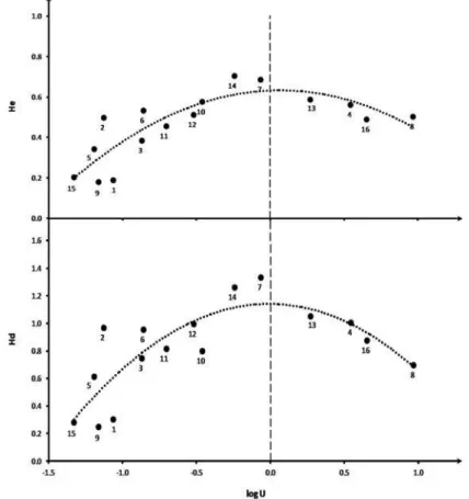
To detect anthropogenic effects, the nature of the patch types should be taken into account. Exchanges in favor of anthropogenic classes such as urban zones or agricultural patch types will reflect a decrease in the degree of naturalness of the landscape. An application of the landscape disturbance index (O’Neill et al.1988; August et al.2002; Barima et al. 2011; Bogaert et al.2011b; Mama et al. 2013) seems useful in this context. It can be used to verify the hypothesis which relates increasing landscape entropy, i.e. spatial compositional heterogeneity, to higher levels of anthropogenic impact (Bogaert et al.2005). Figure8.3shows that max-imum entropy is to be observed at intermediate levels of anthropogenic influence. The aforementioned trends observed by Bogaert et al. (2005) seem to correspond to the upward parts of the curves. The bell-shaped trends in Fig.8.3are not unex-pected: the extremities of the curves correspond to landscapes with high
Fig. 8.2 Landscape pattern is determined by landscape composition (patch type dominance, definition, and richness) and configuration (shapes, sizes, dispersion and densities of patches; patch type juxtaposition). Patch type definition depends on the contrast between patch types
dominance, hence low heterogeneity; in between, equilibrium of anthropogenic and natural types is expected, characterized by higher index values for heterogeneity and evenness. This has noteworthy perspectives since entropy is considered a driver of biodiversity (Fahrig et al.2011).
The transition matrix can be used to simulate future landscape evolution (Urban and Wallin 2002; Barima et al. 2010b, 2011; Vranken et al. 2011;
Fig. 8.3 Impact of anthropogenic landscape disturbance on landscape entropy. Compositional spatial heterogeneity is used as a proxy for landscape entropy and is measured by means of the Shannon evenness index (He) and the Shannon diversity index (Hd). Anthropogenic impact is
measured by a logarithmic transformation of the U disturbance index (O’Neill et al.1988) which is the ratio between the cumulative area of anthropogenic patch types and the cumulative area of natural patch types. Sixteen study zones from classified Landsat TM scenes in the Democratic Republic of the Congo (labels 4, 8, 9, 10, 14, 15, 16) and Benin (labels 1, 2, 3, 5, 6, 7, 11, 12, 13) have been used. A higher dispersion for landscapes dominated by natural land covers is observed; while natural patterns are generally site-specific and rather unique, patterns of urbanization and agricultural development can be site-independent, leading to pattern uniformity across sites within the same cultural area (Bridgewater and Arico2002; Grimm et al.2008). The different relative positions of landscapes in both graphs emphasize the interaction of the number of patch types with evenness
Toyi et al.2013a). To decouple simulations from the time periods characterizing the transition matrix, annual probabilities of landscape change are to be determined. This operation is still subject to debate. The algorithm proposed by Urban and Wallin (2002) could not always be validated (data not shown). The determination of these annual probabilities seems more difficult than expected, and requires a profound mathematical analysis, as shown by Takada et al. (2010).
Patch shape analysis represents a central activity in pattern assessment. Two main analysis types can be distinguished. Firstly, patch shape can be compared to a reference shape, generally an isodiametric one such as a disk or square (Patton
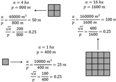
1975; Bogaert et al.2000c; Bogaert2001). This analysis is useful when estimating edge effects, which are proportionally larger for elongated or complex shapes than for isodiametric ones of equal area (Forman and Godron1986; Toyi et al.2013b). The difference between both shapes can then be expressed by means of a perimeter-to-area ratio, obligatory dimensionless to avoid size effects (Fig.8.4). Perimeter-to-area ratios are generally based on the isoperimetric principle, which states that of all shapes with an equal perimeter, the disk is characterized by the largest area (Fig.8.5); the principle could also be interpreted otherwise: of all shapes with an equal area, the disk is characterized by the shortest perimeter. For raster based data, the reference perimeter does not correspond to a circular shape but is a function of the number of pixels composing the patch (Bogaert et al.2000c; Bogaert and Hong
2004).
The second type of shape analysis consists of the determination of the fractal dimension. Since it cannot be determined for a single patch (i.e. when multi-scalar information is not available), a regression technique is applied to estimate it for a group of patches with similar geometry (Krummel et al.1987; Imre and Bogaert
2004; Bamba et al.2009,2010; Bogaert et al.2011b; Colson et al.2011; Diallo et al.2011). The statistical regression parameters can consequently be interpreted to validate this hypothesis; to guide the analyst in its selection, a common origin of the patches, i.e. a common shape-forming process, could be suggested. In case of shape regularity, which indicates anthropogenic effects, the fractal dimension will tend towards one; for increasing patch complexity, associated with natural patch forming processes, fractal dimension will be significantly higher, with two as its upper bound.
A relationship has been shown between patch size and fractal dimension (Krummel et al.1987); larger patches are expected to be characterized by a larger fractal dimension since their shapes are determined by natural patterns, such as geomorphologic discontinuities; small patches are often anthropogenic and even when they are natural, their shape is usually determined by adjacent anthropogenic patches. Nevertheless, it should be noted that aggregation of anthropogenic patches can generate complex patch geometries which could be confounded with natural landscape elements (Fig.8.6).
The dynamics of a patch type can be characterized by the identification of the corresponding transformation process (Forman 1995; Jaeger 2000; Bogaert et al.2004,2008; Koffi et al.2007; Vranken et al.2011). As for a transition matrix, two land cover maps are needed in a diachronic analysis; the analysis is done per
patch type. The current technique has the advantage that it is based on basic pattern information (number of patches, patch type area, patch type perimeter) and that it is applicable to patch types with decreasing or increasing area, hence for natural and anthropogenic types, the latter generally characterized by an increase in their extent in time when anthropogenic effects become more dominant. A second advantage is the availability of a decision tree model which guides the analyst directly to the spatial transformation process for the patch type considered; in order to determine the transformation process, the model uses comparisons of the number of patches, patch type area and patch type perimeter before and after transformation of the type (e.g., Bogaert et al.2004,2008; Barima et al.2009; Diallo et al.2011).
Fig. 8.4 The impact of patch size on patch shape assessment. a is the patch area, p is the patch perimeter. The three square shapes should generate an identical shape index value when their shape is quantified. This is observed for ffiffiffi
a
p =p, which is dimensionless. When a/p is used (a non dimensionless metric), larger patches are characterized by larger values, which is to be avoided
Fig. 8.5 The isoperimetric principle. (a) Circular shape with area ac and perimeter pc. (b)
Irregular shape with perimeterp ¼ pc; consequentlya< ac. (c) Irregular shape with area a ¼ ac;
8.3
Historical Perspective on Anthropogenic Effects
in Landscapes
Anthropogenic effects refer to those land use and land cover dynamics which are caused by human activities. Since Man replaces natural land covers by anthropo-genic ones, and since this substitution is not a random one, landscape pattern can be used to detect anthropogenic influence. Historically, noticeable anthropogenic effects are accepted to be associated with the start of agriculture (Fig.8.8). No other activity has transformed humanity, and the Earth, as much as agriculture (Tilman1998). In ecological terms, agriculture represents a symbiotic relationship between humans and domesticated plants and animals (Cox and Atkins1979). It is evident that also earlier in time, i.e. before the invention of agriculture, anthropo-genic effects should have occurred; however, due to the low population density, the local (or even sub-patch) character of the land cover changes and the non-sedentary character of the populations involved, they can be accepted of little or no signifi-cance. Before the invention of agriculture, it is supposed that Man lived in equi-librium with its environment and that all landscapes were natural landscapes.
Three ages are generally distinguished to subdivide the Holocene: the Paleolithic pre-agricultural era, which ended about 10,000 years BP, the agricultural era, between 10,000 years BP and the industrial revolution (~1800), and the agro-industrial era, since the agro-industrial revolution (Cox and Atkins1979; Smith1989; Gupta 2004; Pinhasi et al. 2005; Sheaffer and Moncada 2009; Balaresque et al. 2010). Landscape-scale dynamics have occurred since man has become sedentary. This change of life style is accepted to have been directly related to
Fig. 8.7 Spatial transformation processes generally observed for natural and anthropogenic patch types.Arrows indicate causal relationships and expected sequences in time. Solid arrows refer to processes characterizing natural patch types.Dashed arrows refer to processes characterizing anthropogenic patch types
the invention of agriculture in the Neolithic era. Early hominids were hunters and gatherers who relied on naturally occurring vegetation, fruits, nuts, carrion and game for subsistence (Gupta 2004; Sheaffer and Moncada 2009). Hunters and gatherers did not establish permanent settlements such as villages. They moved their camps in response to changes in the season and climate (Gupta2004).
Among the most significant examples of human impact on the evolution of ecological niches come from domestication of animals and plants; domestication refers to the process of reciprocation, by which animal and plant species come to depend on humans for survival, while providing humans with numerous benefits in turn (Cox and Atkins1979; Gupta2004). The process of domestication has been markedly important for spatial expansion and population increase of humans during the Holocene (Soja2003; Gupta2004; Sheaffer and Moncada2009). It is however noteworthy that this link between agricultural development and population growth is still subject to debate (Childe 1950; Kohl and Wright 1977; Armelagos et al. 1991). Domesticated species were of prime importance for agriculture: without agriculture, the complex, technically innovative societies and large human populations that exist today could not have evolved (Gupta 2004). Hus-bandry is consequently defined as the cultivation of domesticated plants and
Fig. 8.8 Relationships between the development of agriculture, the evolution of Man’s sedentary lifestyle and landscape change. After a period of hunting and gathering food in which nature and its biomass production were observed, Man developed a sedentary lifestyle through domestication of plants and animals. The natural landscape matrix was consequently replaced by an agricultural one. The use of animal energy enabled Man to increase agricultural productivity, leading to rural exodus and the development of villages and cities. After the industrial revolution, agriculture increasingly integrated with industrial activities. Urban development in recent times was only possible by these earlier developments in husbandry. Urbanization actually introduces new landscape dynamics replacing agricultural landscapes by urban ones
and diversification of the plant communities (Gupta2004; Sheaffer and Moncada
2009).
It is appealing to detail these links between the start of husbandry, the founding of settlements, the development of villages, and the origin of cities. Increasing agricultural productivity is suggested as a key concept in this sequence. While agricultural production itself refers to the total quantity of biomass produced, the productivity concept expresses this quantity as a function of the production factors used (e.g., Van Zanden1991). These factors can be numerous and heterogeneous, such as the time between the preparation of the land and the final yield, the number of farmers involved in production, the production surface used, energy inputs, or the quantities and types of fertilizers used. The nomadic lifestyle of Man before the development of agriculture and its dependence on natural rhythms and production had taught Man to observe and understand its environment. Through this necessity to adapt his life style to nature, Man acquired knowledge on the production of biomass in nature (Braidwood 1979; Sheaffer and Moncada 2009). Later on, agricultural productivity was increased, e.g. by use of energy provided by domes-ticated animals (Demangeon 1933; Childe 1950; Davis 1955; Kohl and Wright
1977; Smith 2009). This enabled individuals to leave the agricultural sector. Through this tendency, the initial agricultural settlements, which were still domi-nated by farmers and their families, were converted into (non-agricultural) villages, and later on, into urbanized zones. Between 6000 and 4000 B.C., certain innova-tions (such as the ox-drawn plow) facilitated, when taken together, a more intensive and more productive use of the Neolithic elements themselves; the rise of cities and towns required in addition to highly agricultural conditions, a form of social organization in which certain strata could appropriate part of the produce grown by the cultivators (Davis1955).
One can agree with the dominant view that the diverse technological innovations constituting the Neolithic culture were necessary to the existence of settled com-munities (Davis1955). Surprisingly, Soja (2003) states that no agricultural surplus was necessary for the development of cities, but that cities were necessary for the
production of an agricultural surplus, at least in certain regions in the world. This hypothesis is denoted a persistent error in the non archeological literature: archeological records show quite clearly and consistently throughout the world that the Neolithic revolution (agriculture) occurred first, and only afterwards did the first cities emerge (Smith2009).
It should be noted that land change to build cities and to support the demands of urban populations itself drives other types of environmental change: urban dwellers depend on the productive and assimilative capacities of ecosystems well beyond their city boundaries (ecological footprint concept), to provide the flows of energy, material goods and nonmaterial services that sustain human well-being and quality of life (Grimm et al.2008; Vranken et al.2011; Seto et al.2012).
Agriculture also evolved throughout history. A tendency towards uniformity (of production systems and crops) on large scales has been observed (Ramade
2005), stimulated, amongst others, by the green revolution (Evanson and Gollin
2003), the sustainability and socioeconomic impacts of which have been criticized. New technologies have been applied, and high levels of energy input have become characteristic for production. The use of energy in multiple farming systems and for different crops has been debated (Cox and Atkins1979; Cleveland1995; Ramade
2005; Gliessman2006; Pimentel and Pimentel2008; Pimentel et al.2008; Pimentel
2009; Sheaffer and Moncada2009); larger energy inputs are not always coupled to higher energy efficiency. Moreover, a shift towards the production of feed and biofuels instead of food has been observed, despite their less favorable energy balance and environmental issues (Pimentel 2003; Pimentel and Patzek 2005; Gliessman 2006; Groom et al. 2008; Pimentel et al.2009). Growing crops for biofuel not only ignores the need to reduce natural resource consumption, but exacerbates the problem of malnourishment worldwide by turning food grain into biofuel (Pimentel et al.2009): this raises major ethical and moral issues (Pimentel
2003; Pimentel and Patzek2005). The aforementioned trends, combined with the increasing demographic pressure, will have profound impacts on landscapes, since larger areas will be required to produce biomass to directly feed humans, to grow livestock, and to provide alternatives for fossil fuels. This potential spatial impact of biofuel production is discussed in Groom et al. (2008).
8.4
Agriculture and Urbanization: Matrix Competitors
Agricultural development from a local, low productive activity to an extensive, high yielding production process based on high energy inputs, has put his footprint on societies and landscapes. Through technical developments and concomitant fossil fuel consumption, one farmer has nowadays become able to produce more per unit area and on larger extents than ever before. Therefore, it can be accepted that agricultural land uses became dominant in landscapes through time and have replaced the original natural patch types, such as forests, by anthropogenic ones, such as fields, fallow lands, pasture lands or agricultural buildings. This tendency,
often detected as deforestation, has been frequently observed (Lepers et al.2005). This increase of patch types related to farming consequently decreased the cumu-lative area of natural areas; often only non fertile areas or difficultly accessible zones such as mountains or swamps were not converted into farmland. Land accessibility is often cited as the main cause of landscape change, next to their intrinsic properties (August et al. 2002). The landscape matrix, which has been dominated exclusively by natural patch types before the arrival of agriculture, was consequently systematically replaced by an anthropogenic, agricultural matrix (Figs8.9 and 8.10). The area increase of the anthropogenic type(s) was mainly caused by patch creation, enlargement and aggregation. The decreasing overall area for the natural patch types was the consequence of perforation, dissection, frag-mentation, shrinkage and attrition.
Not only total patch type area, but also the number of patches per type was influenced by this substitution (Fig.8.11). Initially, both types, natural and anthro-pogenic, were characterized by an increase in their number of landscape elements. This increase could have been expected to be faster for the natural than for the anthropogenic types, since anthropogenic activities, especially farming, are con-sidered to have been more efficient when aggregated in space: short distances between farmlands were preferred and adjacent lands even more. This increase in the number of patches slowed down when patches started aggregating (for anthro-pogenic types) or disappearing (for natural types). When the substitution had continued, finally both types would have been characterized by a low(er) number of patches, and the final frequencies of patches could then be described using the typology of Forman and Godron (1986) categorizing them in disturbance patches, remnant patches, introduced patches and environmental resource patches, according to their origin or cause of existence (Fig.8.12).
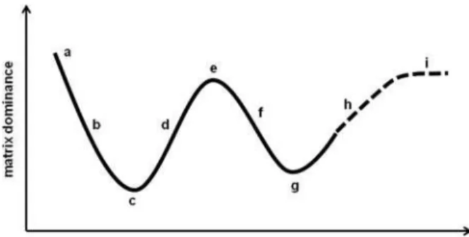
intrinsic urban population growth after an initial period of settlement (d ). Trends shown are not to be interpreted quantitatively, since their magnitudes are not representative and intend to illustrate expected landscape dynamics only. Model mainly inspired on northern hemisphere landscapes
This substitution of a natural matrix (of which the land cover types were mainly determined by the abiotic context, such as the climate or geomorphology) by an agricultural one could have been repeated later on, but this time when an urban matrix was replacing the formerly dominant agricultural one. Urbanization is namely expected to be dominant in contemporary landscapes, with a dominant
Fig. 8.10 Schematic representation of the historical evolution of the landscape matrix in which anthropogenic patch types have become dominant (theoretical model). (a) dominance of the initial natural patch types; (b) decrease of the matrix dominance of natural patch types due to area increase of agricultural patch types; (c) co-dominance of natural and agricultural patch types; (d ) increasing dominance of agricultural patch types; (e) maximum dominance of agricultural patch types; (f ) decrease of agricultural patch types because of substitution by urbanization; (g) co-dominance of urban and agricultural patch types; (h) increasing dominance of urban patch types;i) equilibrium state (hypothesis). Trends shown are not to be interpreted quantitatively, since their magnitudes are not representative and intend to illustrate expected landscape dynamics only. Model mainly inspired on northern hemisphere landscapes
Fig. 8.11 Evolution of patch density when a natural land cover (A) is replaced by an anthropo-genic one (B). Theoretical model of the replacement of a natural landscape matrix by an agricultural one. Initial patch density increase of natural patch types is mainly caused by dissection and fragmentation; the later decrease of patch density is caused by patch attrition. The initial increase of anthropogenic patch density is expected to be caused by patch creation. Due to patch proximity, patch enlargement, and ongoing patch creation, anthropogenic patches are hypothe-sized to aggregate more rapidly to form large contiguous landscape elements forming the land-scape matrix, which decreases patch density of this type. Crossing curves should not be excluded
limited physical extents; this trend has been reversed over the last 30 years with urban areas that are nowadays expanding on average twice as fast than their populations (Seto et al.2012). For the United States, a>30 % of increase of the amount of land devoted to urban and built-up uses between 1982 and 1997 was noted (Alig et al.2004).
Two major pathways of urban impacts on land cover are to be considered. In the developed world, large-scale urban agglomerations and extended peri-urban settle-ments fragment the landscapes of such large areas that various ecosystem processes are threatened; however, ecosystem fragmentation in peri-urban regions may be offset by urban-led demands for conservation and recreational land uses; on the other hand, in less developed countries, urbanization seems to outbid all other uses for land adjacent to the city, including prime croplands (Lambin et al.2001). Urban zones are characterized by rapid enlargement and the management of peri-urban zones, where rural and urban areas meet and conflict, announces itself as a key issue for landscape ecology in the near future, although an unambiguous functional and morphological definition and identification of peri-urban zones remains subject to debate (Fig.8.13) (Forman 2008; Andre´ et al. 2012). These peri-urban environ-ments are the glue that link core cities in extended urbanized regions (Grimm et al.2008): the “edge” of the city expands into the surrounding rural landscape, including changes in soils, built structures, markets, and informal human settle-ments, all of which exert pressure on fringe ecosystems.
Thus, according to the aforementioned landscape dynamics model, which can be denoted as the “nature-agriculture-urban model”, natural landscapes are replaced by anthropogenic ones, initially dominated by agriculture, later on by land covers reflecting urban development. It should be noted, however, that there are different trajectories of land cover change in different parts of the world (e.g., decrease of cropland in temperate areas and increase in the tropics) (Lepers et al.2005). This observation confirms the aforementioned model with tropical countries still expanding their agricultural matrix while in temperate zones the urbanization has
already taken over, although a co-dominance of both agriculture and urbanization should not be excluded. Agricultural development and urbanization are not syn-chronized between developed and developing countries but since both hemispheres seem to follow the same model, the outcome of both evolutions is predictable. In Forman and Godron (1986) a similar, five-step anthropization gradient was presented, with natural, managed, cultivated, suburban and urban landscapes.
8.5
Concluding Commentary: Space Is a Limited Resource
The concept of limited (or not renewable) resources refers to those elements that can be extracted or consumed but for which the available quantity is considered well-defined. When a fraction of the resource is used, the remaining quantity consequently declines. Sometimes, this consumed quantity can be restored after a long period, but the delay is often too long to consider the resource as renewable. This concept of resource limitation can also be applied in landscape ecology. Landscapes are composed of different types of land cover which each occupy a fraction of a geographical space. This geographical space is limited, i.e. it corre-sponds to a well-defined extent. Consequently, space could and should be
Fig. 8.13 Urbanization and agriculture alter the composition and configuration of natural patch types. A disintegration and area decrease of natural patch types is observed and contiguous zones are replaced by isolated patches subject to edge effects. The natural matrix is transformed into a scattered pattern of remnant patches. An anthropogenic matrix dominates now the landscape. Urban growth leads to functional and structural rural-urban conflicts in peri-urban areas
References
Alig RJ, Kline JD, Lichtenstein M (2004) Urbanization in the urban landscape: looking ahead in the 21st century. Landsc Urban Plan 69:219–234
Allen TFH, Starr TB (1982) Hierarchy: perspectives for ecological complexity. University of Chicago Press, Chicago
Alongo S, Visser M, Drouet T et al (2013) Effets de la fragmentation des foreˆts par l’agriculture itine´rante sur la de´gradation de quelques proprie´te´s physiques d’un Ferralsol e´chantillonne´ a` Yangambi, R.D. Congo. Tropicultura 31:36–43
Andre´ M, Mahy G, Lejeune P, et al (2012) Vers une de´finition unique des zones pe´riurbaines ? L’apport de l’e´cologie du paysage pour la segmentation du gradient urbain-rural. In: APERAU (ed) Journe´es APERAU 2012. Penser et Produire la Ville au XXIe`me Sie`cle. Modernisation e´cologique, qualite´ urbaine et justice spatiale. Lausanne
Armelagos GJ, Goodman AH, Jacobs KH (1991) The origins of agriculture: population growth during a period of declining health. Popul Environ 13:9–22
August P, Iverson L, Nugranad J (2002) Human conversion of terrestrial habitats. In: Gutzwiller KJ (ed) Applying landscape ecology in biological conservation. Springer, New York Balaresque P, Bowden GR, Adams SM et al (2010) A predominantly neolithic origin for European
paternal lineages. PLoS Biol 8:e1000285
Bamba I, Mama A, Neuba DFR et al (2008) Influence des actions anthropiques sur la dynamique spatio-temporelle de l’occupation du sol dans la province du Bas-Congo (R.D. Congo). Sci Nat 5(1):49–60
Bamba I, Iyongo Waya Mongo L, Imre A et al (2009) La variabilite´ du facteur de graduation utilise´ dans la me´thode d’estimation de la dimension fractale des mosaı¨ques paysage`res. Ann ISEA Bengamisa 4:168–176
Bamba I, Barima YSS, Bogaert J (2010) Influence de la densite´ de la population sur la structure spatiale d’un paysage forestier dans le bassin du Congo en R. D. Congo. Trop Conserv Sci 3:31–44
Barima YSS, Barbier N, Bamba I et al (2009) Dynamique paysage`re en milieu de transition foreˆt-savane ivoirienne. Bois For Trop 299:15–25
Barima YSS, Barbier N, Ouattara B et al (2010a) Relation entre la composition floristique et des indicateurs de la fragmentation du paysage dans une re´gion de transition foreˆt-savane ivoirienne. Biotechnol Agron Soc Environ 14:617–625
Barima YSS, Egnankou MW, N’Doume´ CTA et al (2010b) Mode´lisation de la dynamique du paysage forestier dans la re´gion de transition foreˆt-savane a` l’est de la Coˆte d’Ivoire. Rev Teledetec 9:129–138
Barima YSS, Djibu JP, Alongo S et al (2011) Deforestation in Central and West Africa: landscape dynamics, anthopogenic effects and ecological consequences. In: Daniels JA (ed) Advances in environmental research, volume 7. Nova Science Publishers, Hauppauge
Bastin JF, Djibu JP, Havyarimana F et al (2011) Multiscalar analysis of the spatial pattern of forest ecosystems in Central Africa justified by the pattern/process paradigm: two case studies. In: Boehm DA (ed) Forestry: research, ecology and policies. Nova Science Publishers, Hauppauge Bogaert J (2001) Size dependence of interior-to-edge ratios: size predominates shape. Acta
Biotheor 49:121–123
Bogaert J, Andre´ M (2013) Landscape ecology: a unifying discipline. Tropicultura 31:1–2 Bogaert J, Impens I (1998) Generating random percolation clusters. Appl Math Comput 91:197–
208
Bogaert J, Mahamane A (2005) Ecologie du paysage: cibler la configuration et l’e´chelle spatiale. Ann Sci Agron Benin 7:1–15
Bogaert J, Van Hecke P, Impens I (1999a) A reference value for the interior-to-edge ratio of isolated habitats. Acta Biotheor 47:67–77
Bogaert J, Van Hecke P, Moermans R et al (1999b) Twist number statistics as an additional measure of habitat perimeter irregularity. Environ Ecol Stat 6:275–290
Bogaert J, Moermans R, Van Hecke P (2000a) Fractal dimension of patches based on area and perimeter: evaluation of the non-regression technique. In: Ceulemans R, Bogaert J, Deckmyn G et al (eds) Topics in ecology: structure and function in plants and ecosystems. University of Antwerp (UIA), Wilrijk
Bogaert J, Rousseau R, Van Hecke P (2000b) Percolation as a model for informetric distributions: fragment size distribution characterized by Bradford curves. Scientometrics 47:195–206 Bogaert J, Rousseau R, Van Hecke P et al (2000c) Alternative area–perimeter ratios for
measure-ment of 2-D shape compactness of habitats. Appl Math Comput 111:71–85
Bogaert J, Van Hecke P, Salvador-Van Eysenrode D et al (2000d) Landscape fragmentation assessment using a single measure. Wildl Soc B 28:875–881
Bogaert J, Salvador-Van Eysenrode D, Impens I et al (2001a) The interior-to-edge breakpoint distance as a guideline for nature conservation policy. Environ Manag 27:493–500
Bogaert J, Salvador-Van Eysenrode D, Hecke V et al (2001b) Land-cover change: quantification metrics for perforation using 2-D gap features. Acta Biotheor 49:161–169
Bogaert J, Salvador-Van Eysenrode D, Van Hecke P et al (2001c) Geometrical considerations for evaluation of reserve design. Web Ecol 2:65–70, Erratum Web Ecol 2:74
Bogaert J, Myneni RB, Knyazikhin Y (2002a) A mathematical comment on the formulae for the aggregation index and the shape index. Landsc Ecol 17:87–90
Bogaert J, Van Hecke P, Ceulemans R (2002b) The Euler number as an index of spatial integrity of landscapes: evaluation and proposed improvement. Environ Manag 29:673–682
Bogaert J, Zhou L, Tucker CJ et al (2002c) Evidence for a persistent and extensive greening trend in Eurasia inferred from satellite vegetation index data. J Geophys Res 107:14. doi:10.1029/ 2001JD001075
Bogaert J, Hong SK (2004) Landscape ecology: monitoring landscape dynamics using spatial pattern metrics. In: Hong SK, Lee JA, Ihm BS (eds) Ecological issues in a changing world. Status, response and strategy. Kluwer, Dordrecht
Bogaert J, Ceulemans R, Salvador-Van Eysenrode D (2004) A decision tree algorithm for detection of spatial processes in landscape transformation. Environ Manag 33:62–73 Bogaert J, Farina A, Ceulemans R (2005) Entropy increase of fragmented habitats signals human
impact. Ecol Indic 5:207–212
Childe VG (1950) The urban revolution. Town Plann Rev 21:3–17
Cleveland CJ (1995) Resource degradation, technical change, and the productivity of energy use in U.S. agriculture. Ecol Econ 13:185–201
Colson F, Bogaert J, Carneiro Filho A et al (2009) The influence of forest definition on landscape fragmentation assessment in Rondoˆnia, Brazil. Ecol Indic 9:1163–1168
Colson F, Bogaert J, Ceulemans R (2011) Fragmentation in the Legal Amazon, Brazil: can landscape metrics indicate agricultural policy differences? Ecol Indic 11:1467–1471 Costanza R, d’Arge R, de Groot R et al (1997) The value of the world’s ecosystem services and
natural capital. Nature 387:253–260
Coulson RN, Saarenmaa H, Daugherty WC et al (1999) A knowledge system environment for ecosystem management. In: Klopatek JM, Gardner RH (eds) Landscape ecological analysis. Issues and applications. Springer, Berlin
Cox GW, Atkins MD (1979) Agricultural ecology. An analysis of world food production systems. W.H. Freeman and Company, San Francisco
Dale VH, Fortes DT, Ashwood TL (2002) A landscape-transition matrix approach for land management. In: Lui J, Taylor WW (eds) Integrating landscape ecology into natural resource management. Cambridge University Press, Cambridge
Davis K (1955) The origin and growth of urbanization in the world. Am J Sociol 60:429–437 Deblauwe V, Barbier N, Couteron P et al (2008) The global biogeography of semi-arid periodic
vegetation patterns. Glob Ecol Biogeogr 17:715–723
Deblauwe V, Couteron P, Lejeune O et al (2011) Environmental modulation of self-organized periodic vegetation patterns in Sudan. Ecography 34:990–1001
Deblauwe V, Couteron P, Bogaert J et al (2012) Determinants and dynamics of banded vegetation pattern migration in arid climates. Ecol Monogr 82:3–21
Demangeon A (1933) Villages et communaute´s rurales. Ann Geogr 42:337–349
Diallo H, Bamba I, Barima YSS et al (2011) Effets combine´s du climat et des pressions anthropiques sur la dynamique e´volutive de la ve´ge´tation d’une zone prote´ge´e du Mali (Re´serve de Fina, Boucle du Baoule´). Se´cheresse 22:97–107
Diouf A, Barbier N, Mahamane A et al (2010) Caracte´risation de la structure spatiale des individus ligneux dans une « brousse tachete´e » au sud-ouest du Niger. Rev Can Rech For 40:827–835 Diouf A, Barbier N, Lykke AM et al (2012) Relationships between fire history, edaphic factors and woody vegetation structure and composition in a semi-arid savanna landscape (Niger, West Africa). Appl Veg Sci 15:488–500
Ellis EC, Ramankutty N (2008) Putting people in the map: anthropogenic biomes of the world. Front Ecol Environ. doi:10.1890/070062
Evanson RE, Gollin D (2003) Assessing the impact of the green revolution, 1960 to 2000. Science 300:758–762
Fahrig L (2005) When is a landscape perspective important? In: Wiens JA, Moss M (eds) Issues and perspectives in landscape ecology. Cambridge University Press, Cambridge
Fahrig L, Baudry J, Brotons L et al (2011) Functional landscape heterogeneity and animal biodiversity in agricultural landscapes. Ecol Lett 14:101–112
Farina A (2000a) Principles and methods in landscape ecology. Kluwer Academic, Dordrecht Farina A (2000b) Landscape ecology in action. Kluwer Academic, Dordrecht
Farina A, Bogaert J, Schipani I (2005) Cognitive landscape and information: new perspectives to investigate the ecological complexity. Biosystems 79:235–240
Fischer J, Lindenmayer DB (2007) Landscape modification and habitat fragmentation: a synthesis. Glob Ecol Biogeogr 16:265–280
Forman RTT (1995) Land mosaics. The ecology of landscapes and regions. Cambridge University Press, Cambridge
Forman RTT (2008) Urban regions. Ecology and the planning beyond the city. Cambridge University Press, Cambridge
Forman RTT, Godron M (1986) Landscape ecology. Wiley, New York
Gliessman SR (2006) Agroecology. The ecology of sustainable food systems. CRC Press, Boca Raton
Grimm NB, Faeth SH, Golubiewski NE et al (2008) Global change and the ecology of cities. Science 319:756–760
Groom MJ, Gray EM, Townsend PA (2008) Biofuels and biodiversity: principles for creating better policies for biofuel production. Conserv Biol 22:602–609
Gupta AK (2004) Origin of agriculture and domestication of plants and animals linked to early Holocene climate amelioration. Curr Sci 87:54–59
Havyarimana F, Bogaert J, Ndayishimiye J et al (2013) Impact de la structure spatiale de Strombosia scheffleri Engl. et Xymalos monospora (Harv.) Baill. sur la re´ge´ne´ration naturelle et la coexistence des espe`ces arborescentes dans la re´serve naturelle forestie`re de Bururi, Burundi. Bois For Trop 316:49–61
Hobbs RJ, Hopkins JM (1990) From frontier to fragments: European impact on Australia’s vegetation. Proc Ecol Soc Aust 16:93–114
Hufkens K, Bogaert J, Dong QH et al (2008) Impacts and uncertainties of upscaling of remote-sensing data validation for a semi-arid woodland. J Arid Environ 72(2008):1490–1505 Imre AR, Bogaert J (2004) The fractal dimension as a measure of the quality of habitats. Acta
Biotheor 52:41–56
Imre AR, Bogaert J (2006) The Minkowski-Bouligand dimension and the interior-to-edge ratio of habitats. Fractals 14:49–53
Iyongo Waya Mongo L, Visser M, De Cannie`re C et al (2012) Anthropisation et effets de lisie`re: impacts sur la diversite´ des rongeurs dans la Re´serve Forestie`re de Masako (Kisangani, R.D. Congo). Trop Conserv Sci 5:270–283
Iyongo Waya Mongo L, De Cannie`re C, Ulyel J et al (2013) Effets de lisie`re et sex-ratio de rongeurs forestiers dans un e´cosyste`me fragmente´ en Re´publique De´mocratique du Congo (Re´serve de Masako, Kisangani). Tropicultura 31:3–9
Jaeger J (2000) Landscape division, splitting index, and effective mesh size: new measures of landscape fragmentation. Landsc Ecol 15:115–130
Koffi KJ, Deblauwe V, Sibomana S et al (2007) Spatial pattern analysis as a focus of landscape ecology to support evaluation of human impact on landscapes and diversity. In: Hong SK, Nakagoshi N, Fu B et al (eds) Landscape ecological applications in man-influenced areas. Linking man and nature systems. Springer, Dordrecht
Kohl P, Wright RP (1977) Stateless cities: the differentiation of societies in the near eastern Neolithic. Dialect Anthropol 2:271–283
Krummel JR, Gardner RH, Sugihara G et al (1987) Landscape patterns in a disturbed environment. Oikos 48:321–324
O’Neill RV, Krummel JR, Gardner RH et al (1988) Indices of landscape pattern. Landsc Ecol 3:153–162
Patton DR (1975) A diversity index for quantifying habitat “edge”. Wildl Soc B 3:171–173 Pimentel D (2003) Ethanol fuels: energy balance, economics, and environmental impacts are
negative. Nat Resour Res 12:127–134
Pimentel D (2009) Energy inputs in food crop production in developing and developed nations. Energies 2:1–24
Pimentel D, Patzek TW (2005) Ethanol production using corn, switchgrass, and wood; biodiesel production using soybean and sunflower. Nat Resour Res 14:65–76
Pimentel D, Pimentel M (2008) Food, energy, and society. CRC Press, Boca Raton
Pimentel D, Wilson C, McCullum C et al (1997) Economic and environmental benefits of biodiversity. Bioscience 47:747–757
Pimentel D, Williamson S, Alexander CE et al (2008) Reducing energy inputs in the US food system. Hum Ecol 36:459–471
Pimentel D, Marklein A, Toth MA et al (2009) Food versus biofuels: environmental and economic costs. Hum Ecol 37:1–12
Pinhasi R, Fort J, Ammerman AJ (2005) Tracing the origin and spread of agriculture in Europe. PLoS Biol 3:2220–2228
Rakotondrasoa OL, Malaisse F, Rajoelison GL et al (2013) Identification des indicateurs de de´gradation de la foreˆt de tapia (Uapaca bojeri) par une analyse sylvicole. Tropicultura 31:10–19
Ramade F (2005) Ele´ments d’e´cologie applique´e. Dunod, Paris
Reino L, Beja P, Osborne PE et al (2009) Distance to edges, edge contrast and landscape fragmentation: Interactions affecting farmland birds around forest plantations. Biol Conserv 142:824–838
Salvador-Van Eysenrode D, Bogaert J, Van Hecke P et al (1998) Influence of tree-fall orientation on canopy gap shape in an Ecuadorian rain forest. J Trop Ecol 14:865–869
Salvador-Van Eysenrode D, Kockelbergh F, Bogaert J et al (2002) Canopy gap edge determination and the importance of gap edges for plant diversity. Web Ecol 3:1–5
Seto KC, Gu¨neralp B, Hutyra LR (2012) Global forecasts of urban expansion to 2030 and direct impacts on biodiversity and carbon pools. Proc Natl Acad Sci U S A 109:16083–16088 Sheaffer CC, Moncada KM (2009) Introduction to agronomy: food, crops and, environment.
Delmar Cengage Learning, Clifton Park
Smith ME (2009) V. Gordon Childe and the urban revolution: a historical perspective on a revolution in urban studies. Town Plann Rev 80:3–29
Soja EW (2003) Putting cities first: remapping the origins of urbanism. In: Bridge G, Watson S (eds) A companion to the city. Blackwell, Oxford
Stepp JR, Castaneda H, Cervone S (2005) Mountains and biocultural diversity. Mt Res Dev 25:223–227
Takada T, Miyamoto A, Hasegawa SF (2010) Derivation of a yearly transition probability matrix for land-use dynamics and its applications. Landsc Ecol 25:561–572
Tilman D (1998) The greening of the green revolution. Nature 396:211–212
Toyi MS, Barima YSS, Mama A et al (2013a) Tree plantation will not compensate natural woody vegetation cover loss in the Atlantic Department of Southern Benin. Tropicultura 31:62–70 Toyi MS, Bastin JF, Andre´ M et al (2013b) Effets de lisie`re sur la productivite´ du teck (Tectona
grandis L.f.): e´tude de cas des teckeraies prive´es du Sud-Be´nin. Tropicultura 31:71–77 Tratalos J, Fuller RA, Warren PH et al (2007) Urban form, biodiversity potential and ecosystem
services. Landsc Urban Plan 83:308–317
Turner MG (1989) Landscape ecology: the effect of pattern on process. Annu Rev Ecol Syst 20:171–197
Turner MG, Gardner RH, O’Neill RV (2001) Landscape ecology in theory and practice. Pattern and process. Springer, New York
Urban DL, Wallin DO (2002) Introduction to Markov models. In: Gergel SE, Turner MG (eds) Learning landscape ecology. A practical guide to concepts and techniques. Springer, New York Urban DL, O’Neill RV, Shugart HH Jr (1987) Landscape ecology. A hierarchical perspective can
help scientists understand spatial patterns. Bioscience 37:119–127
Van Peer L, Nijs I, Bogaert J et al (2001) Survival, gap formation, and recovery dynamics in grassland ecosystems exposed to heat extremes: the role of species richness. Ecosystems 4:797–806
Van Zanden JL (1991) The first green revolution: the growth of production and productivity in European agriculture, 1870–1914. Econ Hist Rev 44:215–239
Vranken I, Djibu Kabulu JP, Munyemba Kankumbi F et al (2011) Ecological impact of habitat loss on African landscapes and diversity. In: Daniels JA (ed) Advances in environmental research, volume 14. Nova Science Publishers, Hauppauge
Vranken I, Amisi YM, Munyemba FK et al (2013) The spatial footprint of the non-ferrous mining industry in Lubumbashi. Tropicultura 31:20–27
Watling JI, Orrock JL (2010) Measuring edge contrast using biotic criteria helps define edge effects on the density of an invasive plant. Landsc Ecol 25:69–78
Wiens JA (2009) Introduction: framing the issues. In: Collinge SK (ed) Ecology of fragmented landscapes. Johns Hopkins University Press, Baltimore