All authors: Université Laval, Department of Economics, Pavillon J.-A.-DeSève, Québec, QC, Canada G1V 0A6; and CIRPÉE
Bellemare: [email protected] Bissonnette: [email protected] Kröger: [email protected]
Part of the paper was written at the Institute of Finance at the School of Business and Economics at Humboldt Universität zu Berlin and at the Department of Economics at Zurich University. We thank both institutions for their hospitality. We thank Nicolas Couët for his valuable research assistance. We are grateful to participants at the ASFEE conference in Montpellier (2012), ESA meeting in New York (2012), the IMEBE in Madrid (2013), and seminar participants at the Department of Economics at Zurich University (2013) and at Technische Universität Berlin (2013).
Cahier de recherche/Working Paper 14-25
Statistical Power of Within and Between-Subjects Designs in
Economic Experiments
Charles Bellemare Luc Bissonnette Sabine Kröger
Abstract:
This paper discusses the choice of the number of participants for within-subjects (WS) designs and between-subjects (BS) designs based on simulations of statistical power allowing for different numbers of experimental periods. We illustrate the usefulness of the approach in the context of field experiments on gift exchange. Our results suggest that a BS design requires between 4 to 8 times more subjects than a WS design to reach an acceptable level of statistical power. Moreover, the predicted minimal sample sizes required to correctly detect a treatment effect with a probability of 80% greatly exceed sizes currently used in the literature. Our results suggest that adding experimental periods in an experiment can substantially increase the statistical power of a WS design, but have very little effect on the statistical power of the BS design. Finally, we discuss issues relating to numerical computation and present the powerBBK package programmed for STATA. This package allows users to conduct their own analysis of power for the different designs (WS and BS), conditional on user specified experimental parameters (true effect size, sample size, number of periods, noise levels for control and treatment, error distributions), statistical tests (parametric and nonparametric), and estimation methods (linear regression, binary choice models (probit and logit), censored regression models (tobit)).
Keywords: Within-subjects design, Between-subjects design, sample size, statistical
power, experiments
1
Introduction
Researchers planning an experimental study have to decide about the number of subjects, treatments, experimental periods to employ and whether to conduct a within or between-subjects design. All these decisions require a careful balancing between the chance of finding an existing effect and the precision with which this effect can be measured.1 For
example, subjects taking part in a within-subjects (WS hereafter) design are exposed to several treatment conditions while subjects in a between-subjects (BS hereafter) design are exposed to only one. WS designs thus offer the possibility to test theories at the individual level and can boost statistical power, making it more likely to correctly reject a null hypothesis in favor of an alternative hypothesis. They can, however, also gen-erate spurious treatment effects, notably order effects. BS designs, on the other hand, can attenuate order effects but may have lower statistical power as we illustrate in this paper. Charness, Gneezy, and Kuhn (2012) summarize the tradeoff between both designs by saying: “Choosing a design means weighing concerns over obtaining potentially spu-rious effects against using less powerful tests.”(p.2.) In addition, the number of subjects and the number of periods (McKenzie, 2012) affect the statistical power of a study. As a result, understanding the statistical power of WS and BS designs in relation to sample size and periods is an essential step in the process of designing economic experiments.
More generally, recent work has raised awareness about the relationship between power of statistical tests and optimal experimental designs (e.g., List, Sadoff, and Wagner (2011); Hao and Houser (forthcoming)). Yet, statistical power remains largely undis-cussed or reported in published experimental economic research. Zhang and Ortmann (2013), for example, reviewed all articles published in Experimental Economics between 2010 and 2012 and fail to find a single study discussing optimal sample size in relation to statistical power.2 We conjecture that this can partly be explained by the incompati-1The former influence is referred to in the literature as the power of a study, that is the probability
of not rejecting the Null hypothesis when in fact it is false, in other words of not committing a Type II error. The latter influence refers to the width of the confidence interval, i.e., the conviction with which we are confident not committing a Type I error, i.e., rejecting the Null hypothesis when in fact it is true.
bility of existing power formulas derived under very specific conditions with experimental data. The formulas are not adapted for the diversity of experimental data (with WS and BS designs; discrete, continuous, and censored outcomes; multiple periods; non-normal errors) nor are they available for the variety of statistical tests (nonparametric and para-metric) used in the literature. This incompatibility poses challenges to experimentalists interested in predicting power for the designs they consider. As a result, researchers may unknowingly conduct underpowered experiments which lead to a waste in scarce resources and potentially guide research in unwanted directions.3
The main objective of this paper is to provide experimental economists with a simple unified framework to compute ex-ante power of an experimental design (WS or BS) using simulation methods. Simulation methods are general enough to be used in conjunction with a variety of statistical tests (nonparametric and parametric), estimation methods (for linear and non-linear models), and samples sizes used in experimental economics. It can also easily handle settings with non-normal errors. Conversely, closed form expressions for statistical power computation are typically derived for simple statistical models and tests and tend to be valid under specific conditions (e.g., large sample sizes, normally distributed errors). For other conditions, power computation using closed form expressions may overestimate the level of power in finite samples (see, e.g., Feiveson, 2002). The simulation approach to power computation is simple and well known in applied statistics and can help researchers determine the number of subjects, the number of periods, and the design (WS or BS) required to reach an acceptable level of statistical power. In this paper we focus on simulating the statistical power of a test for the null hypothesis of no treatment effect against a specific alternative.4 For our simulations, we consider a population of
economics, and applies more widely to other fields such as education (Brewer and Owen, 1973), market-ing (Sawyer and Ball, 1981), and various sub-fields in psychology (Mone, Mueller, and Mauland, 1996; Cohen, 1962; Chase and Chase, 1976; Sedlmeier and Gigerenzer, 1989; Rossi, 1990).
3Long and Lang (1992) reviewed 276 articles (not necessarily experimental) published in top journals
in economics and proposed a method to estimate the share of papers falsely failing to reject the null hypothesis. Their estimates suggest that all non-rejection results in their sample of articles are false, a consequence of low statistical power.
agents whose outcome variable is generated using a possibly non-linear panel data model which depends on a binary treatment variable, individual unobserved heterogeneity, and idiosyncratic shocks. From this population, researchers sample subjects and assign them to either treatment or control over several periods. In this setup a BS design assigns subjects to either treatment or control conditions for all periods while a WS design assigns subjects to a minimum of one period to both treatment and control conditions. We look at both balanced and unbalanced WS designs – subjects in a balanced WS design are observed for the same number of periods under both treatment conditions while subjects in an unbalanced design are observed for different number of periods on both treatment conditions. Additionally, we look at the relationship between the statistical power of both designs and the number of experimental periods. All other aspects of the model (treatment effect sizes and noise parameters) require calibration using data from existing economic experiments.
We illustrate the approach in the context of gift exchange experiments and calibrate our model using data from two existing field experiments. We find that the BS design re-quires approximately 4 times more subjects than the WS design to reach acceptable levels of power (80%) when the number of experimental periods is small (2 periods). Power of the WS design is found to increase substantially with the number of experimental periods. Power of the BS design is found to be less sensitive to an increase in experimental periods. As a result, the BS design requires approximately 12 times more subjects compared to a WS design when the number of experimental periods is larger (6 periods). We find that these results are relatively robust to the true treatment effect sizes. Increasing the noise level requires a larger sample size in both designs, however, the ratios become less large. Then, the BS design requires approximately 3 times more observations with a low number of periods and 6 times more when the number of experimental periods is larger. Our analysis suggests that the number of subjects needed to reach an acceptable level of power in this research area can be large. For example, we find that minimal sample sizes required to reach a power of 80% with a BS design range from 232 to 1054 subjects under our low noise scenario and range from 458 to 2200 subjects under our high noise scenario.
Corresponding sample sizes with a WS design ranged from 20 to 218 subjects under our low noise scenario and ranged from 66 to 738 subjects for our high noise scenario.
Finally, we present the powerBBK package for STATA that we developed to simulate power with the needs of economists in mind. This package allows to simulate the minimal necessary sample size to reach a user-specified level of statistical power or to compute the statistical power of a particular design, given information on sample size, variances, and minimal detectable effect size. The package can handle panel data and can be used for non parametric (e.g., Wilcoxon Sign test or Mann-Whitney-U test) and parametric tests. It can also be used in the context of linear regression models with or without normal errors, binary response models (probit and logit) and censored regression models (tobit). The paper is organized as follows. Section 2 presents a brief survey of the experimental parameters used in recent articles published in Experimental Economics, the top field journal for experimental work in economics, to illustrate typical sample sizes and design choices employed in this field. Section 3 discusses the simulation of statistical power and introduces the powerBBK package. Section 4 presents our application to gift exchange. Section 5 concludes.
2
Brief survey of experimental designs in
Experi-mental Economics
In this section we present a brief analysis of sample sizes and design choices of all papers published in Experimental Economics in volumes 15 and 16 (2012 and 2013). We focus on three aspects affecting statistical power: the choice of experimental design (WS vs. BS), the average number of subjects per treatments and the distribution of the subjects across treatments. In the two volumes we surveyed, a total of 71 papers were published. Our analysis focus on papers with original data and which provided sufficient information to determine the number of subjects in each treatments, leaving us with a sample of 58 papers (36 in 2012, 22 in 2013).
designs. In some cases where elements of both designs are applied, we classified the papers as mixed design. The first two columns of Table 2 present the frequency of each type of designs in each year.
We see from this table that the majority of the paper (41 out of 58) used a BS design. The central part of Table 2 reports some summary statistics on the number of treatments and active subjects per treatments (e.g., excluding receivers who do not take decisions in a dictator game). The table provides mean, median, minimum and maximum values. The following analysis is based on the median, as this measure is less sensitive to outliers. We find that the median number of treatments amongst papers using a BS design is 3 with a median number of subjects of 43.5. These values are respectively 2 and 50 for papers using a WS design, and 4 and 66 for papers using mixed designs.
In the following, we illustrate how those studies divide the total number of their participants across the various treatments. We separate studies in two groups: those where the allocation of subjects to treatments was based on equal repartition and those where repartition is unequal. To proceed, we allow for some small differences in group size when deciding wether a study relied on equal repartition or not by using a simple rule. For instance, a problem would arise with a study in which an odd number of subjects has to be divided into two treatment groups, as it would necessarily lead to a unequal repartition under a strict equality condition. Suppose that you have N subjects to split in T treatments. Denote N\T the integer division of N by T (e.g., 10\3 = 3) We consider that a study used an equal repartition when treatment sizes fall in the interval defined by N\T − 1 and N\T + T − 1. Consider a case with 100 subjects to be split over r 4 treatments. Any study where treatment sizes fall between 24 and 28 subjects would then be considered as one with an equal repartition of subjects. While this simple rule is certainly ad hoc, we found that it leads to a classification very close to our intuitive judgment when looking at the distribution of subjects in a study. The last part of Table 2 presents our classification using this rule. We find that 59% percent of studies using a BS design and 75% of studies using a WS design are classified as using an equal repartition of subjects.
Design Y ear Num b er of treatmen ts Sub jects p er treatmen t Equal repartition 2012 2013 T otal Median Mean Min Max Median Mean Min Max P ercen t Bet w een 26 15 41 3 3.2 2 6 43.5 77.0 18.7 420.3 59% Within 4 4 8 2 2.4 2 4 50.0 73.6 13.5 175.5 75% Mixed 6 3 9 4 4.4 2 12 66 81 29 150 56% T otal 36 22 58 3 3.2 2 12 51 77.2 13.5 420.3 60% T able 1: Summary statistics of exp erimen tal parameters used in articles published in Exp erimental Ec onomics in v olumes 15 and 16 (2012 and 2013).
Several observations emerge from the analysis above. First, the BS design is predom-inantly used. Second, the number of subjects does not seem to be related to the choice of design (WS or BS), despite the fact that WS design tend to be more powerful (as il-lustrated in the following section). Third, assigning the same number of subjects to each treatment appears to be a dominant practice. This hints that assignment of subjects to treatments was not done in a way that would maximize the statistical power of the test, but rather on other concerns.5
It is important to emphasize that the results presented here do not imply that exper-iments we surveyed are underpowered. Even if we would be interested in computing the statistical power of those studies as reference point of the statistical power in the litera-ture, we could not do so as in many cases, at least one information necessary to compute statistical power (e.g., variance of treatment and control outcomes) was not reported.
3
Power in regression models
Our analysis is based on the following treatment effect regression model
y∗it= β0+ β1dit+ µi+ ϵit (1)
where yit∗ denotes the latent outcome variable of subject i at period t, dit is a binary
treatment variable taking a value of 1 when subject i receives treatment at period t and 0 otherwise, µi represents time-invariant unobserved heterogeneity with the cumulative
distribution function Fµ. The remaining errors ϵit are drawn from a cumulative
distri-bution Fϵ|d(a). We allow the errors to be heteroscedastic : the variance of the errors
5We also pursued more informal ways to learn about the usage of power analysis in experimental
economics, e.g., the ESA mailing list and searching for results of power analysis reported by experimental studies published in economic journals. Outcomes were not conclusive given the low number of observa-tions. We found only two studies reporting results of ex-ante power analysis used to compute minimal necessary sample sizes (Rutstr¨om and Wilcox, 2009; Ferraro and Price, 2013) and a handful of studies conducting ex-post power analyses to determine whether absence of statistical significance can be related to low sample sizes (Smith, Williams, Bratton and Vonnoni, 1982; Bossaerts, Plott and Zame, 2007; Voors et al 2012; Trautmann, van de Kuilen, and Zeckhauser, 2013; Stoop, 2014).
ϵit can depend on treatment conditions dit. Let σϵ,02 and σ2ϵ,1 denote the variance of ϵit
under control and treatment conditions respectively. We maintain the assumption that
µi is independent of dit. This assumption is typically motivated by the randomization
of subjects to treatment conditions. It is possible to relax this assumption and allow for some dependance between µi and dit(letting for example the variance of µi vary with the
treatment). It is also possible to add other regressors to (1). Implementing these changes requires minor adjustments to the simulation algorithm presented below, but for the sake of exposition, we focus on the simple specification.
The observable outcome variable yit may differ from y∗it. We consider three leading
cases.
Case 1. yit = yit∗ - a linear model
Case 2. yit = 1 if yit∗ ≥ 0, and 0 otherwise - a binary choice model Case 3. yit = max(a, y∗it) - a model with censoring from below at a
We assume throughout that β1 does not vary across the population, but this could be
easily relaxed. This parametrization allows us to generate samples for different sequences
{dit : t = 1, 2, . . . , T} given values of (β0, β1) and (Fµ, Fϵ|d). Identification of (β0, β1)
requires some minimal restrictions on the functions (Fµ, Fϵ|d). Mean independence with
the treatment indicator is sufficient for the linear model (Case 1). Independence between
ϵit is typically assumed for Cases 2 and 3. Note that Cases 1 and 3 allow the variance of
ϵit to differ between control and treatment conditions. The probit and logit models result
from setting Fϵ to the standard normal and logistic distribution respectively for Case 2.
Setting Fϵ|d to mean zero normal distribution with variance σϵ,d2 in Case 3 leads to the
tobit model. The distribution Fµ is often assumed to be a normal distribution with mean
zero and variance σ2
µ.
A BS design implies that {dit : t = 1, 2, . . . , T} does not vary across t, a subject
is either assigned only to the control condition (dit = 0 for all t) or to the treatment
condition (dit = 1 for all t). In the presence of homoscedastic errors ϵit, the noise level
µi + ϵit is the same for treatment and control conditions. In this case it is reasonable to
conditions. In the presence of heteroscedastic errors ϵit, statistical power can possibly be
improved by assigning more subjects to the conditions where the noise level is higher. A WS design implies that {dit: t = 1, 2, . . . , T} varies across t for each subject. In the
presence of homoscedastic errors ϵit, it is reasonable to use a balanced WS design with
dit = 0 for T /2 periods. In the presence of heteroscedastic errors ϵit, statistical power
may be improved by assigning subjects to the more noisy conditions for a higher number of periods.
3.1
Power computation
It is straightforward to compute power curves using the following steps.
Step 1. Fix N and T and generate for a given design (WS or BS) a sample {{(yit, dit) :
t = 1, . . . , T} : i = 1, 2 . . . , N} given values of (β0, β1) and choice of (Fµ, Fϵ).
Step 2 - parametric. Estimate (β0, β1) and the parameters of (Fµ, Fϵ|d) and compute
ˆ
z = ˆβ1/se( ˆβ1) and the corresponding p-value of the null hypothesis H0 : β1 = 0 against
either a one-sided or two-sided alternative. Here se( ˆβ1) denotes the standard error of the
estimate.6
Step 2 - nonparametric. Aggregate the individual data over T and use nonparametric
rank-based tests (e.g., Wilcoxon rank-sum test for BS data, Wilcoxon signed-rank test for WS data) of the null hypothesis that the distribution of the aggregated values of y are the same under control and treatment conditions and compute the p-value of the test.
Step 3. Repeat steps 1 and 2 for a large number of samples. Compute the fraction of p-values which are less than the significance level of the test (e.g., 5%). This represents
the power of the test.
Repeating the three steps above for a range of N and T values for each design, enables the researcher to plot power curves. Power curves are useful for comparing the designs
6Note, that the estimators used in step 2 will depend on the nature of the outcome variable. The
maximum likelihood estimator can be used in all three cases. Linear regression with clustered standard errors can also be used in the case of the linear model. This is a popular choice for experimental economists, as the distributions (Fµ, Fϵ|d) are often unknown in practice.
for a given sample size, for determining the minimal sample size needed to reach a certain statistical power separately for each design, or to look at the effect of the number of periods and how to balance the number of participants in the treatments.
Simulations can be conducted using any statistical software which integrates Monte Carlo simulations (e.g., GAUSS, OX, Matlab, STATA). We developed a user-friendly pack-age for STATA users called powerBBK packpack-age that executes Steps 1 to 3 for given values of
β1, σ2µ, σϵ2, etc. It was designed with flexibility in mind and can be used to simulate power
for a class of popular data-generating processes encountered in experimental economics using a single command line. The powerBBK package is provided as an .ado file along with a help file and can be downloaded here (http://www.ecn.ulaval.ca/en/luc.bissonnette). As expected, powerBBK requires the user to specify details concerning the experimental design, such as the number of subjects, number of periods, WS or BS design, balance of WS design and so on. There are options to evaluate the statistical power over a range of values N and to assess simultaneously power of both WS and BS designs. The user can specify whether or not to include individual heterogeneity by means of random-effects terms (i.e., the variance of µi is greater than 0) or to include treatment-specific
het-eroscedasticity (i.e., the variance of ϵit depends on the treatment received). Users can
also specify the distribution of errors (Fµ, Fϵ|d) they require for their simulations, thus
allowing for example heavy-tailed distributions in linear models. The package further allows to simulate power of nonparametric rank-based tests and can accommodate sev-eral common non-linear models (i.e., logit, probit, tobit).7 Additional information and
examples are available in the help-file provided with the package.
4
Illustration : gift exchange in the field
When possible, researchers planning new experiments can perform an ex-ante power analy-sis using data from pilot experiments conducted in the exact setting where the experiment is scheduled to take place. Alternatively, they can perform their power analysis using data
7In those cases, the distributions are (F
from other related studies. We illustrate the power analysis presented in section 3 with an application in the context of field experiments designed to measure reciprocal pref-erences of workers. Our analysis exploits data from two different studies in this area. Gneezy and List (2006) use a BS design in the context of a single day spot labor market experiment with a data entry task. They assign 9 workers to their treatment condition (gift) and 10 workers to the control condition (no gift). They estimate a linear random-effects panel data model (Case 1 in Section 3) with individual specific random-effects µi and where
t indexes the hour of work within the experimental day. Bellemare and Shearer (2009)
use a WS design with 18 subjects. They test how workers (tree-planters) respond to a gift from their employer. Their WS design is unbalanced : workers planted first for 5 days under control conditions (no gift). Workers then received a gift on the final day of planting on the experimental block. Bellemare and Shearer (2009) estimate a linear fixed-effects panel data model (Case 1) with individual specific effects µi and where t
indexes the day of work during the experiment. Both studies use roughly the same total number of subjects and time periods, but the notion of time varies across studies.
We first estimated a random-effects panel data model of equation (1) using the Gneezy and List data with the dependent variable being the natural lof of productivity. We get ( bβ0, bβ1) = (3.674, 0.055), bσ2µ= 0.088, bσ2ϵ = 0.018. The corresponding estimates using the
Bellemare and Shearer data are ( bβ0, bβ1) = (6.955, 0.061), bσ2µ = 0.046, bσ2ϵ = 0.018. The
estimated treatment effect (β1) and estimated error variance σϵ2 are very similar for both
studies. The estimated value of σ2
µ(unobserved heterogeneity) on the other hand is twice
as high in the Gneezy and List data.8
We next used the estimated model parameters from both datasets to simulate power of WS and BS designs for two scenarios. The low noise scenario sets (σ2
µ = 0.045 and 8Both studies estimate regression models using the variable y
itin level – they do not use the natural
logarithm of productivity as the dependent variable. Using the natural logarithm of productivity sim-plifies the comparison of the estimated treatment effect of both studies. Bellemare and Shearer (2009) additionally control for weather effects while Gneezy and List (2006) allow the effect of the gift to vary across time. Estimated model parameters with those additional controls are very similar to the results we report here.
σ2
ϵ = 0.02 while the high noise scenario sets σ2µ= 0.09 and σϵ2 = 0.02. The variance of µi
in the high noise scenario is thus exactly twice the corresponding value for the low noise scenario. We will consider three values for β1 (0.05, 0.1 and 0.15) for both scenarios. The
value of β0 plays no role in our analysis and will be set to 6.3 in all our simulations. We
will also consider setting T to 2 and 6. Setting T = 6 proxies the number of time periods used in both studies used for our calibration. The case T = 2 is interesting because it proxies experiments which take place on a single day while still allowing a meaningful comparison of WS and BS designs.9 It also represents a case where researchers have little information to control for the presence of unobserved individual heterogeneity µi. It is
straightforward to consider other values of T . We perform a separate power analysis for each scenario for a double-sided test with a 5% level of significance. We implement the BS design by assigning the same number of subjects to control and treatment conditions. We implement a balanced WS design by assigning subjects to the same number of periods under control and treatment conditions. We also simulated power for an “unbalanced” WS design assigning subjects to the treatment condition for only one out of six time periods. Simulated power of the unbalanced WS design was not very different to power of the balanced WS we report here. This is to be expected as the variance of the outcome variable is kept constant under control and trial conditions. We thus focus our analysis on the balanced WS design. Finally, we use the OLS estimator with standard errors clustered at the individual level. All our results are very similar when using the (asymptotically more efficient) GLS estimator.
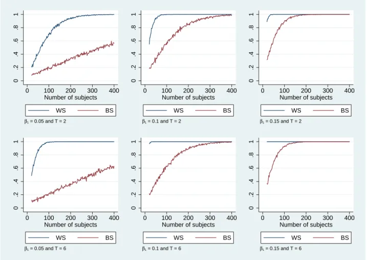
Figure 1 presents the simulated power curves for the low noise scenario. Several regularities emerge. First, we find that power is systematically higher for the WS design for all 6 combinations of β1 and T values used. This result is expected given the WS
design exploits within-subject variation in decisions for a given individual (for a given level of µi). This advantage of the WS design over the BS design is well documented (see,
e.g., Keren (1993)). We also find that increasing the number of periods raises power of the WS design but has relatively minor impact on power of the BS design. The quantitative
differences in power between both designs are perhaps more surprising. A natural way to compare both designs is to compare the minimal number of subjects (MNS) required to reach a given level of power. Social scientists often argue that an experiment should aim to correctly detect a treatment effect 80% of the time (see Cohen, 1988) when using a double-sided test along with a 5% significance level. Table 2 presents the simulated MNS required to reach this power threshold derived from the curves in Figure 1. We find that the MNS exceeds 400 subjects for the BS design for both values of T when β = 0.05. In comparison, the MNS of the WS design is 122 subjects when T = 2, and 42 subjects when T = 6. As expected, the required MNS decrease with β. The MNS of the BS design when β = 0.1 are 182 subjects and 162 subjects for 2 and 6 periods respectively. The corresponding MNS of the WS design are 30 subjects and less than 20 subjects, thus 6 to 8 times less than the corresponding MNS of the BS design. Finally, MNS of the BS when
β = 0.15 are 84 subjects and 74 subjects for 2 and 6 periods respectively. Corresponding
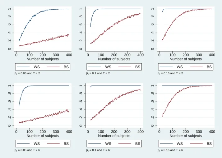
MNS of the WS design are both below 20 subjects, roughly 4 time less than the BS design. Figure 2 presents the simulated power curves for the high noise scenario. Several interesting regularities emerge. First, power curves of the WS design in the high noise scenario are very similar to those of the WS in the low noise scenario. Power of the BS design on the other hand is substantially worse under the high noise scenario than under the low noise scenario. These regularities are captured by the corresponding MNS of both designs (see Table 2). We find that the MNS of the WS in the high noise scenario are very similar to the corresponding values in the low noise scenario. The MNS of the BS design on the other hand and considerably higher. In particular, we find that the BS design requires between 286 and 302 subjects to detect a value of β = 0.1 with power of 80%. This is roughly 120 subjects more (approx. 65% more) than required in the low noise scenario. Similarly, we find that MNS of the BS design lays between 130 and 140 subjects when β1 = 0.15. This is roughly 60 subjects more (approx. 70% more) than required
in the low noise scenario. These results suggest that researchers planning to conduct BS design experiments in this area should carefully consider the level of noise they expect to be present in the data.
Finally, we repeated the power analysis using nonparametric rank based tests. We used the Wilcoxon rank-sum test when testing for the presence of a treatment effect under BS designs, and used the Wilcoxon signed-rank test under WS designs. Both tests maintain that distributions of y (averaged over T ) for control and treatment conditions are the same under the null. Table 2 presents the simulated MNS for both designs. All results are very similar to those of Table 2, suggesting that they are robust to the test used given the assumed data-generating process.10
5
Conclusion
Underpowered experimental designs can have important consequences for the representa-tiveness of published experimental research (Fanelli and Ioannidis, 2013). In particular, it may result in publication bias if papers failing to detect a significant treatment effect face a lower acceptance probability in academic journals (Button et al., 2013; Nosek, Spies, and Motyl, 2012). This in turn may discourage researchers from even submitting papers reporting insignificant treatments effects, leading to a waste of limited resources.
Our brief survey of design practices of the experiments published in the 2012 and 2013 volumes of Experimental Economics suggests that current practice in experimental economics to determine the sample size is based on other concerns rather than statistical power. Given the advantages of power analysis, the lack of attention to power analysis when designing an experiment might be surprising.
Several reasons have been put forward to explain why the applied statistics literature in general does not systematically discuss power. First, assessing statistical power is more complex than deciding on significance levels. Conceptually, it requires to stipulate an alternative hypothesis with an anticipated effect size, or at least a minimal effect size below which it is not worth the effort conducting the study. Second, researchers may have developed other ways to decide upon the sample size. Sawyer and Ball (1981) conducted
10Simulated power curves of both rank based tests are also very similar to those presented in Figures
a survey amongst researchers and suggest as one reason that researchers rely on their intuition and experience when determining the sample size and the design of a study rather than computing statistical power. However, relying on intuition might lead astray even high profile statisticians. Tversky and Kahneman (1971) observed that researchers who were well trained in statistics often had wrong intuition about the sample size necessary to conduct a replication study. Finally, (un)awareness of statistical power or the publishing culture can be responsible for the lack of power analysis. Mone, Mueller, and Mauland (1996) for example examine the perception of statistical power usage amongst researchers in psychology and find relatively little concern for statistical power.
In response to those reasons, the current study aims at raising awareness among exper-imental economists about the effects of design choice on statistical power. We propose to compute ex-ante power using standard simulation methods which can be easily adapted to various econometric models and statistical tests. Additionally, we present a flexible STATA package (powerBBK) which can be used to perform these simulations.
It is important to emphasize that the advantage of the high flexibility of the simulation approach to conduct proper power analysis for follow-up studies comes at the expense of some knowledge of the underlying data generating process to calibrate the necessary pa-rameters. One source of such information are existing experimental results. The common practice of sharing collected experimental data either via journal websites or directly be-tween experimental economists is one way of gaining access to such information. Some researchers advocate compulsory checklists before submitting manuscripts to journals for publication (e.g., Simmons, Nelson, and Simonsohn, 2011; Nosek, Spies, and Motyl, 2012) to standardize reported statistics and to counter the problem that published articles rarely provide all necessary information that are required to perform ex-ante power analysis for follow-up studies. Alternatively, when previous results are not available, running pilot ex-periments represents another way to gather information on the data-generating process, which can be used to predict the sample size and the design required to detect various possible treatment effects with sufficient power.
by calibrating the model parameters using data from two studies in this area. Our analysis has focused on minimal sample sizes required to detect an existing treatment effect with a power of 80%. Our results suggest that BS designs in field experiments on gift-giving can require between 4 to 8 times more subjects than the WS design to reach a power of 80%. The BS design was particularly sensitive to the noise levels present in the data we considered. Corresponding nonparametric tests provide very similar results. We note that our illustration was purposefully simple and more complex simulations (binary choice, censored or interval regression, models with heteroscedasticity) can be performed using the same basic principle.
Ex-ante power analysis requires a separate analysis for each setting using different values of the model parameters. Thus, the simulation results reported in this paper cannot be directly extrapolated to other experimental settings. They demonstrate however that the differences in minimal sample sizes required between both designs can be sizable, and that there are important differences in the ability to raise power by increasing sample sizes or adjusting the number of periods.
By focusing on statistical power, we also purposefully neglected other potentially im-portant pros and cons of both designs which require consideration when implementing an experiment. The relative importance of these pros and cons is again context specific. WS designs for example can induce treatment order effects and demand effects, both of which are undesirable. Yet, implementing a WS may seem more natural in settings where there is a natural ordering of the treatment conditions (Greenwald, 1976). BS designs -by construction- are not affected by order effects, but they are not immune to demand effects. Ultimately it is up to researchers to weigh the pros and cons of each design for their specific experimental context.
Lo w noise scenario High noise scenario β = 0 .05 β = 0 .1 β = 0 .15 β = 0 .05 β = 0 .1 β = 0 .15 Betwe en-subje cts design T = 2 > 400 182 84 > 400 302 140 T = 6 > 400 162 74 > 400 286 130 Within-subje cts design T = 2 122 30 < 20 122 34 < 20 T = 6 42 < 20 < 20 44 < 20 < 20 T able 2: Minimal sample sizes required to reac h a p o w er of 80% for a double-sided test with 5% significance lev el (GLS estimator). Sim ulations for the lo w noise scenario based on v alues σ 2 µ = 0 .045 and σ 2 ϵ = 0 .02. Sim ulations for the high noise scenario based on v alues σ 2 µ = 0 .09 and σ 2 ϵ = 0 .02. Results for the BS design are computed b y allo cating the same n um b er of sub jects to con trol and treatmen t conditions. Results for the WS design are computed b y assigning sub jects to the same n um b er of con trol and treatmen t p erio ds.
Lo w noise scenario High noise scenario β = 0 .05 β = 0 .1 β = 0 .15 β = 0 .05 β = 0 .1 β = 0 .15 Betwe en-subje cts design T = 2 > 400 174 84 > 400 318 150 T = 6 > 400 158 72 > 400 306 140 Within-subje cts design T = 2 130 36 < 20 134 34 < 20 T = 6 46 < 20 < 20 46 < 20 < 20 T able 3: Minimal sample sizes required to reac h a p o w er of 80% for a double-sided test with 5% significance lev el. The Wilco xon rank-sum test is used to compute p o w er of the BS design. The Wilco xon signed-rank test is used for the WS design. Sim ulations for the lo w noise scenario based on v alues σ 2 µ = 0 .045 and σ 2 ϵ = 0 .02. Sim ulations for the high noise scenario based on v alues σ 2 µ = 0 .09 and σ 2 ϵ = 0 .02. Results for the BS design are computed b y allo cating the same n um b er of sub jects to con trol and treatmen t conditions. Results for the WS design are computed b y assigning sub jects to the same n um b er of con trol and treatmen t p erio ds.
0 .2 .4 .6 .8 1 0 100 200 300 400 Number of subjects WS BS β1 = 0.05 and T = 2 0 .2 .4 .6 .8 1 0 100 200 300 400 Number of subjects WS BS β1 = 0.05 and T = 6 0 .2 .4 .6 .8 1 0 100 200 300 400 Number of subjects WS BS β1 = 0.1 and T = 2 0 .2 .4 .6 .8 1 0 100 200 300 400 Number of subjects WS BS β1 = 0.1 and T = 6 0 .2 .4 .6 .8 1 0 100 200 300 400 Number of subjects WS BS β1 = 0.15 and T = 2 0 .2 .4 .6 .8 1 0 100 200 300 400 Number of subjects WS BS β1 = 0.15 and T = 6
Figure 1: Simulated statistical power of BS and WS designs with T = 2 and T = 6 for the low noise scenario. Simulations based on values σµ2 = 0.045 and σϵ2 = 0.02. Results for the BS design are computed by allocating the same number of subjects to control and treatment conditions. Results for the WS design are computed by assigning subjects to the same number of control and treatment periods.
0 .2 .4 .6 .8 1 0 100 200 300 400 Number of subjects WS BS β1 = 0.05 and T = 2 0 .2 .4 .6 .8 1 0 100 200 300 400 Number of subjects WS BS β1 = 0.05 and T = 6 0 .2 .4 .6 .8 1 0 100 200 300 400 Number of subjects WS BS β1 = 0.1 and T = 2 0 .2 .4 .6 .8 1 0 100 200 300 400 Number of subjects WS BS β1 = 0.1 and T = 6 0 .2 .4 .6 .8 1 0 100 200 300 400 Number of subjects WS BS β1 = 0.15 and T = 2 0 .2 .4 .6 .8 1 0 100 200 300 400 Number of subjects WS BS β1 = 0.15 and T = 6
Figure 2: Simulated statistical power of BS and WS designs with T = 2 and T = 6 for the high noise scenario. Simulations based on values σµ2 = 0.09 and σ2ϵ = 0.02. Results for the BS design are computed by allocating the same number of subjects to control and treatment conditions. Results for the WS design are computed by assigning subjects to the same number of control and treatment periods.
References
Bellemare, C., and B. Shearer (2009): “Gift giving and worker productivity: Evi-dence from a firm-level experiment,” Games and Economic Behavior, 67(1), 233–244.
Bossaerts, P., C. Plott, and W. R. Zame (2007): “Prices and Portfolio Choices in Financial Markets: Theory, Econometrics, Experiments,” Econometrica, 75(4), 993– 1038.
Brewer, J., and P. Owen (1973): “A Note on the Power of Statistical Tests in the ”Journal of Educational Measurement”,” Journal of Educational Measurement, 10(1), 71–74.
Button, K. S., J. P. A. Ioannidis, C. Mokrysz, B. A. Nosek, J. Flint, E. S. J. Robinson, andM. R. Munafo (2013): “Power failure: why small sample size under-mines the reliability of neuroscience.,” Nature Reviews Neuroscience, 14(5), 365–376.
Charness, G., U. Gneezy, and M. A. Kuhn (2012): “Experimental methods: Between-subject and within-subject design,” Journal of Economic Behavior &
Organi-zation, 81, 1–8.
Chase, L., and R. Chase (1976): “A statistical power analysis of applied psychological research.,” Journal of Applied Psychology.
Cohen, J. (1962): “The statistical power of abnormal-social psychological research: A review,” Journal of abnormal and social psychology, 65(3), 145–153.
(1988): Statistical power analysis for behavioral sciences, 2nd edition. Routledge Academic, New Jersey.
Fanelli, D., and J. P. A. Ioannidis (2013): “US studies may overestimate effect sizes in softer research,” Proceedings of the National Academy of Sciences, 110(37), 15031–15036.
Feiveson, A. (2002): “Power by simulation,” Stata Journal.
Ferraro, P. J., and M. K. Price (2013): “Using nonpecuniary strategies to influence behavior evidence from a large-scale field experiment,” The Review of Economics and
Statistics, 95(1), 64–73.
Gneezy, U., and J. A. List (2006): “Putting Behavioral Economics to Work: Testing for Gift Exchange in Labor Markets Using Field Experiments,” Econometrica, 74(5), 1365–1384.
Greenwald, A. G. (1976): “Within-Subjects Designs: To Use or Not To Use?,”
Hao, L., and D. Houser (forthcoming): “Adaptive Procedures for Wilcoxon-Mann-Whitney Tests: Seven Decades of Advances,” Communications in Statistics: Theory
and Methods.
Keren, G. (1993): “Between- or Within-Subjects Design: A Methodological Dilemma,” in A Handbook for Data Analysis in the Behavioral Sciences, ed. by G. Keren, and
C. Lewis, p. Chapter 8. Lawrence Erlbaum Associates Inc., New Jersey.
List, J., S. Sadoff, and M. Wagner (2011): “So You Want to Run an Experi-ment, Now What? An Introduction to Optimal Sample Arrangements,” Experimental
Economics, 14, 439–457.
Long, J. D., and K. Lang (1992): “Are all economic hypotheses false?,” Journal of
Political Economy, 100(6), 1257–1272.
McKenzie, D. (2012): “Beyond baseline and follow-up : The case for more T in exper-iments,” Journal of Development Economics, 99(2), 210–221.
Mone, M., G. Mueller, and W. Mauland (1996): “The perceptions and Usage of Statistical Power in Applied Psychology and Management Research,” Personnel
Psy-chology.
Nosek, B. a., J. R. Spies, and M. Motyl (2012): “Scientific Utopia: II. Restructur-ing Incentives and Practices to Promote Truth Over Publishability,” Perspectives on
Psychological Science, 7(6), 615–631.
Rossi, J. (1990): “Statistical power of psychological research: what have we gained in 20 years?,” Journal of Consulting and Clinical Psychology, 58, 646–656.
Rutstr¨om, E. E., and N. T. Wilcox (2009): “Stated beliefs versus inferred beliefs: A methodological inquiry and experimental test,” Games and Economic Behavior, 67, 616–632.
Sawyer, A., and A. Ball (1981): “Statistical power and effect size in marketing research,” Journal of Marketing Research, XVIII(August), 275–290.
Sedlmeier, P., and G. Gigerenzer (1989): “Do studies of statistical power have an effect on the power of studies?,” Psychological Bulletin, 105(2), 309–316.
Simmons, J., L. Nelson,andU. Simonsohn (2011): “False-positive psychology undis-closed flexibility in data collection and analysis allows presenting anything as signifi-cant,” Psychological science.
Smith, V. L., A. W. Williams, W. K. Bratton, and M. G.Vannoni (1982): “Competitive Market Institutions: Double Auctions vs. Sealed Bid-Offer Auctions,”
Stoop, J. (2014): “From the lab to the field: envelopes, dictators and manners,”
Exper-imental Economics, 17(2), 304–313.
Trautmann, S. T., G. van de Kuilen,and R. J. Zeckhauser (2013): “Social Class and (Un)Ethical Behavior: A Framework, With Evidence From a Large Population Sample,” Perspectives on Psychological Science, 8(5), 487–497.
Tversky, A., and D. Kahneman (1971): “Belief in the law of small numbers.,”
Psy-chological bulletin.
Voors, M. J., E. E. M. Nillesen, P. Verwimp, E. H. Bulte, R. Lensink, and
D. P. Van Soest (2012): “Violent Conflict and Behavior: A Field Experiment in Burundi,” American Economic Review, 102(2), 941–64.
Zhang, L., and A. Ortmann (2013): “Exploring the Meaning of Significance in Ex-perimental Economics,” UNSW Australian School of Business . . . .