Analyse de la rupture dynamique fragile via les modèles d'endommagement à gradient : principes variationnels et simulations numériques

HAL Id: tel-01487449

https://pastel.archives-ouvertes.fr/tel-01487449

HAL is a multi-disciplinary open access archive for the deposit and dissemination of sci-entific research documents, whether they are pub-lished or not. The documents may come from teaching and research institutions in France or abroad, or from public or private research centers.

L’archive ouverte pluridisciplinaire HAL, est destinée au dépôt et à la diffusion de documents scientifiques de niveau recherche, publiés ou non, émanant des établissements d’enseignement et de recherche français ou étrangers, des laboratoires publics ou privés.

d’endommagement à gradient : principes variationnels et

simulations numériques

Tianyi Li

To cite this version:

Tianyi Li. Analyse de la rupture dynamique fragile via les modèles d’endommagement à gradient : principes variationnels et simulations numériques. Mécanique des solides [physics.class-ph]. Université Paris-Saclay, 2016. Français. �NNT : 2016SACLX042�. �tel-01487449�

THÈSE DE DOCTORAT

DE

L’UNIVERSITÉ PARIS-SACLAY

PRÉPARÉE À

L’ÉCOLE POLYTECHNIQUE

ÉCOLE DOCTORALE N°579

Sciences mécaniques et énergétiques, matériaux et géosciences

Spécialité de doctorat : Mécanique des solides

Par

Monsieur Tianyi LI

Gradient Damage Modeling of Dynamic Brittle Fracture

Variational Principles and Numerical Simulations

Thèse présentée et soutenue à Palaiseau, le 6 octobre 2016 Composition du Jury :

M. Gilles DAMAMME Directeur de recherche, CEA/DAM Président du Jury

M. Alain COMBESCURE Professeur émérite, INSA de Lyon Rapporteur

M. Corrado MAURINI Professeur, Université Pierre et Marie Curie Rapporteur Mme Laura DE LORENZIS Prof. Dr.-Ing., TU Braunschweig Examinatrice M. Jean-Jacques MARIGO Professeur, Ecole Polytechnique Directeur de thèse M. Daniel GUILBAUD Ingénieur de recherche, CEA Saclay Co-encadrant M. Serguei POTAPOV Ingénieur de recherche, EDF Lab Paris-Saclay Co-encadrant

Introduction

Une bonne tenue mécanique des structures du génie civil en béton armé sous chargements dynamiques sévères est primordiale pour la sécurité et nécessite une évaluation précise de leur comportement en présence de propagation de fissures dynamiques. Dans ce travail, on se focalise sur la modélisation constitutive du béton assimilé à un matériau élastique-fragile endommageable en tension seulement. La rupture fragile s’accompagne de très peu de déformations loin de fissures et d’une localisation du tenseur des déformations le long des fissures. La modélisation et l’analyse décrites dans cette étude s’appliquent aux matériaux fragiles vérifiant ces comportements à la rupture.

Une étude bibliographique sur la rupture dynamique fragile est proposée dans le chapitre 1. Plusieurs modèles physiques sont comparés quant à leur aptitude à modéliser la rupture fragile : la théorie classique de Griffith, l’approche variationnelle de la rupture et les modèles d’endommagement à gradient formulés initialement dans un cadre quasi statique. Plusieurs objectifs de cette présente étude sont classifiés en fonction de l’approche utilisée (théorique ou numérique) et en utilisant les sujets thématiques suivants

• Vers la dynamique,

• Établir un lien avec les approches « champ de phase »,

• Meilleure compréhension des modèles d’endommagement à gradient, et • Validation expérimentale.

Modèles d’endommagement à gradient en dynamique

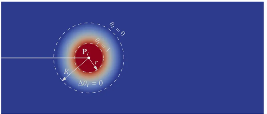
Le chapitre 2 regroupe les contributions théoriques de cette these. On postule que l’évolution spatio-temporelle de la localisation des déformations dans un solide fragile est régie par un modèle d’endommagement à gradient. Il consiste à introduire un nouveau champ scalaire 0 ≤ αt ≤ 1 réalisant

une description régularisée entre la partie saine de la structure αt =0 et la région fissurée αt =1.

Γt Ω αt= 0 αt= 1 O (`) `/L = 10% `/L = 5% `/L = 1% L

On propose une formulation variationnelle des modèles d’endommagement à gradient en dynamique à l’aide de trois principes physiques d’irréversibilité, de stabilité et de bilan d’énergie

1. Irréversibilité : l’endommagement t ↦→ αt est non-décroissant du temps.

2. Stabilité d’ordre un : la variation première de l’action est non-negative par rapport aux évolutions arbitraires et admissibles du couple déplacement-endommagement

A′(u, α)(v − u, β − α) ≥ 0 for all v ∈ C(u) and all β ∈ D(α). iii

H_t = H0+ ∫ t 0 (∫ Ω (σs·ε( ÛUs) −ρ Ûus · ÜUs)dx − Ws( ÛUs) − ÛWs(us) ) ds + ∫ Ω ρ( Ûut· ÛUt− Ûu0· ÛU0)dx

où l’énergie totale est définie par

H_t = E(ut, αt) + S(αt) + K( Ûut) − Wt(ut).

Il s’agit d’une extension en dynamique du formalisme existant en statique via la variation de l’intégrale temporelle d’un lagrangien généralisé prenant en compte l’énergie cinétique K et aussi l’énergie dissipée S due au processus d’endommagement. Grâce au caractère variationnel de la formulation, ces modèles d’endommagement permettent de rendre compte de toute l’évolution de la fissuration avec des trajets et topologies complexes et non-présupposés d’un point de vue modélisation de l’évolution du défaut.

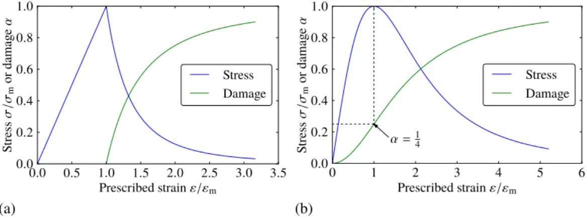
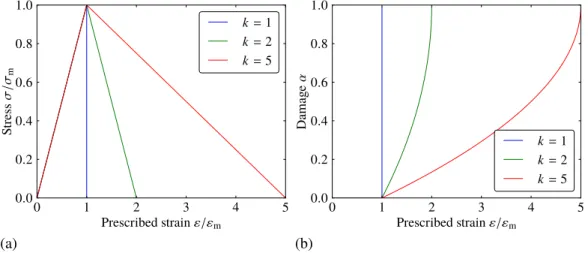
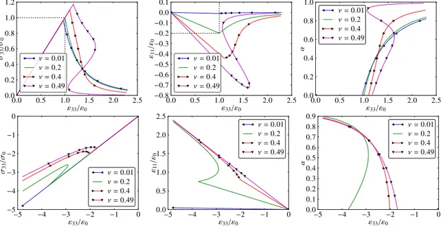
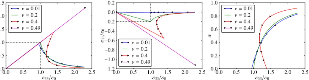
Pour modéliser le comportement asymétrique des matériaux fragiles en traction et en compression, plusieurs formulations basées sur la dépendance de l’énergie élastique vis-à-vis de l’endommagement sont revues et un cadre unificateur est proposé via un principe variationnel. Ces modèles sont vus comme un paramètre matériau en soi décrivant différents mécanismes d’endommagement déterminés par la microstructure. Une meilleure compréhension de leur comportement est obtenue via un essai de traction/compression unidimensionnel.

On s’intéresse ensuite à l’équation d’évolution de fissures régularisées par le champ d’endommage-ment durant la phase de propagation. On démontre que la pointe de la fissure dynamique est régie par un critère de Griffith faisant intervenir le taux de restitution d’énergie dynamique conventionnel Gαt =

∫

Ω\Γt

(

( κ( Ûut)−ψ(ε(ut), αt) )div θt+σt·(∇ut∇θt)+div(ft⊗θt)·ut+ ρÜut·∇utθt+ ρ Ûut·∇ Ûutθt) dx,

et le taux de dissipation d’endommagement γt = ∂ ∂lt S∗(α∗_t,lt) = ∫ Ω\Γt ( ς(αt, ∇αt)div θt−qt · ∇θt∇αt)dx.

La démonstration et la dérivation rigoureuse de ces concepts dans le modèle d’endommagement reposent sur les techniques de dérivation lagrangienne par rapport au domaine basée sur la configuration fissurée initiale et une séparation d’échelles lorsque la longueur interne est petite par rapport à la taille de la structure.

Implémentation numérique

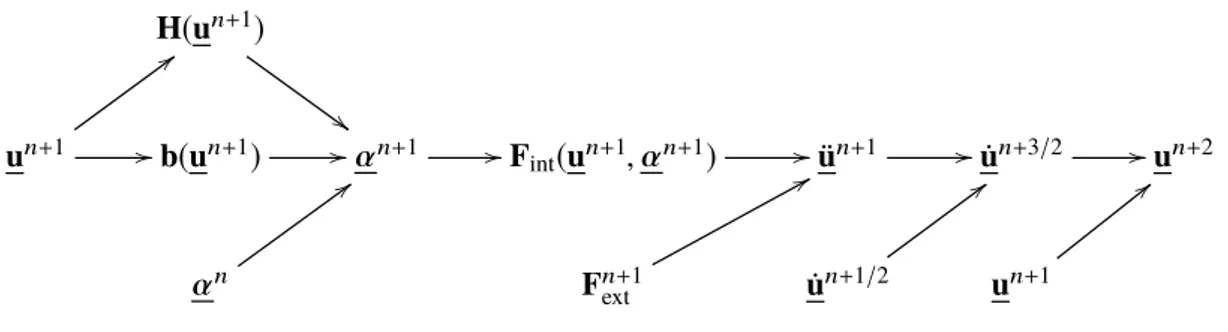
Le caractère variationnel de l’approche permet aussi une implémentation numérique directe et de manière consistante pour des problèmes bi et tri-dimensionnels, cf. le chapitre3. Elle est basée sur une discrétisation par éléments finis standards en espace et le schéma de β-Newmark en temps. Le problème d’endommagement qui détermine l’état de fissuration à l’instant actuel est résolu à l’échelle de la structure par la méthode du gradient conjugué projeté. L’architecture informatique est basée sur la librairie d’algèbre linéaire numérique PETSc qui assure une gestion uniforme des vecteurs et des matrices lors d’un calcul séquentiel ou parallèle. Dans le cas explicite, le modèle discrétisé résumé par l’algorithme suivant est implémenté dans le code de dynamique rapide EuroPlexus, cf. (CEA & EC, 2015)

1: for chaque pas de temps n ≥ 0 do 2: M-à-j Ûun+1/2 = Ûun+ ∆t₂uÜn.

4: Obtenir α via la minimisation d’énergie. 5: Obtenir Üun+1via l’équilibre dynamique. 6: M-à-j Ûun+1= Ûun+1/2+ ∆t₂uÜn+1.

7: end for

Une implémentation open source est aussi disponible dans le code d’éléments finis FEniCS, voir (Li, 2015).

Simulations numériques

Les résultats de simulation obtenus issu des calculs parallèles sont alors discutés d’un point de vue numérique et physique dans le chapitre4. L’efficacité du modèle numérique est démontrée via une analyse de scalabilité. On montre en particulier que la résolution du problème d’endommagement à l’échelle

1 2 4 8 16 Number of cores 0 50 100 150 200 250 300 350 400 450 Time (minutes)

MPI calculation with 106_elements

Perfect scaling Elastodynamics Damage assembly Damage solving Communication 52% 32% 16% 48% 37% 12% 47% 36% 13% 46% 31% 13% 42% 30% 13%

de la structure n’est pas pénalisante pour un calcul explicite de fissuration fragile dynamique. Les lois constitutives d’endommagement et les formulations d’asymétrie en traction et en compression sont comparées quant à leur aptitude à modéliser la rupture fragile. On confirme que la loi d’endommagement intégrant une zone purement élastique est préférable aussi d’un point de vue numérique. Pour un comportement asymétrique en traction et en compression, le modèle basé sur la décomposition spectrale (contraintes/déformations principales) inscrit dans le cadre variationnel du chapitre2permettrait de mieux modéliser la rupture des matériaux fragiles. Cela permettrait un rapprochement avec les modèles « champ de phase » issue de la communauté mécanique numérique.

Pour mieux comprendre les approches d’endommagement à gradient en dynamique en tant qu’un modèle de rupture per se, on adopte une stratégie « divide ut regnes » et leurs propriétés spécifiques sont analysées séparément pour différentes phases de l’évolution du défaut : nucléation, initiation, propagation, arrêt, branchement et bifurcation.

Initiation

Propagation

Nucleation

Branching

Arrest

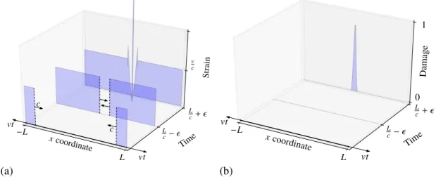
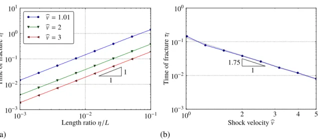
En particulier, la nucléation d’une fissure dans un solide sain est régie par un critère en contrainte accompagné des effets d’échelle introduits par la longueur interne. Cela est illustré par les simulations d’une barre sous choc et d’un essai brésilien sur un cylindre sous compression.

0 5 10 15 20 25 30 Time t/tref 0.0 0.2 0.4 0.6 0.8 1.0 1.2 Applied force F /Fref D= 200 mm

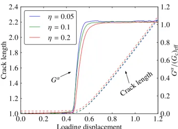
Via un calcul antiplan d’une plaque, on vérifie que la propagation de fissure satisfait la loi de Griffith démontrée dans le chapitre2. Une analyse numérique de convergence vers le modèle quasi-statique y

0.0 0.5 1.0 1.5 2.0 2.5 Loading speed k/c 0.2 0.4 0.6 0.8 1.0 Crac k speed ˙ l/c

Shear wave speed c =pµ/ρ

Num. Theo.

(a)

Quasi-static crack speed vQS= pµH/Gc

Num. Theo.

(b)

Quelques observations numériques au tour d’un zoom spatio-temporel des phénomènes de branchement ou de bifurcation sont décrites et on propose une comparaison avec des critères classiques en mécanique de la rupture. α∗ P0 Pt_c Micro-branching Macro-branching

Des confrontations avec les résultats expérimentaux sont aussi réalisées afin d’évaluer le modèle et proposer des axes d’amélioration. En particulier, on envisage d’utiliser les lois d’endommagement plus sophistiquées pour pouvoir contrôler la bande d’endommagement pour le béton.

Research Background and Outline

From a modeling point of view, the present work concerns the formulation of mathematical models of the physical phenomenon in an industrial context. Due to the complexity of the problem, numerical simulation is also needed to provide an approximate solution of the previous theoretical models. To ensure the faithfulness of the numerically discretized computer model with respect to the theoretical one, the verification step should be first carried out in terms of numerical convergence properties. Finally, validation of the physical and the numerical models will be achieved via the comparison between simulation results and experimental observations. All these steps are covered in the present study.

In civil engineering, mechanical performance and integrity of the reinforced concrete structures are of paramount importance for safety. Severe transient dynamic loading conditions (such as impact or explosion) often lead to crack nucleation and its further space-time evolution in the most vulnerable area, which results in ultimate structural failure. A better understanding of the mechanics of defects would thus guide the civil engineers to optimize the dimensioning, the shape and the topology of the initial design. An accurate assessment of structural behaviors in the presence of dynamic crack propagation calls for more advanced physical models and their corresponding efficient computer implementations. In this aspect, the present work contributes thus to an improvement of the existing modeling of fracture in industrial structures, both from theoretical and numerical approaches.

Numerical simulation of reinforced concrete structures requires in general a separate modeling of the concrete, the reinforcement and the steel-concrete interaction. Due to the broadness of the subject, we will only focus here on the fracture behaviors of concrete itself. A coupling with the existing steel reinforcement models and in particular the phenomenon of interfacial fracture will be thoroughly investigated in the future. The mechanical behaviors of concrete fall into the category of brittle materials. Defect evolution in these materials with dynamical or inertia effects are commonly studied in the branch “dynamic fracture” of physics of solids. Very little deformation is present away from the fractured region and the strain tensor is essentially localized along the crack band. Without loss of generality, the methodology, modeling and analyses described in the present work should apply to a large class of materials that can be characterized by such constitutive and fracture behaviors.

Concretely, the mathematical modeling of dynamic brittle fracture will be performed in the framework of solid continuum mechanics with the usual Cauchy stress as the main stress measure. Adopting an engineering approach, we concentrate on a macroscopic phenomenological characterization of the constitutive behavior of brittle materials in the presence of fracture. In particular, the spatial and temporal evolution of strain localization in a brittle solid will be modeled by the gradient-damage approach that is gaining popularity in the recent years. It consists of introducing a new spatial scalar field αtthat indicates and tracks the location of cracks. It can be considered as a damage variable since

αt =0 refers to an intact material point whereas αt =1 stands for a totally damaged region, i.e. a crack

or a strain-localization area. Compared to other existing approaches of dynamic fracture, the advantage of such gradient damage models lies in the crack path prediction with arbitrary crack topologies from a theoretic defect evolution modeling point of view. Its variational formulation also permits a direct and consistent numerical implementation both for two-dimensional and three-dimensional problems.

A brief bibliographical study of dynamic brittle fracture is provided in Chapter1. We describe first the kinematics and physics of fracture in brittle materials with inertia, since the objective consists of faithfully and efficiently charactering those phenomena. In order to motivate the present work and

variational approach to fracture originated from the pioneer work of (Francfort & Marigo, 1998) and the current gradient damage model formulated in the quasi-static setting (Pham & Marigo, 2010b). Based on the literature investigation, the objectives of the present work can then be defined. They are classified depending on the methodology used (theoretical or numerical approach) and using the following four thematic subjects

• Going dynamical,

• Bridging the link with phase field approaches,

• Better understanding of gradient damage modeling of fracture, and • Experimental validation.

To facilitate the presentation, the main novelty brought by the present study will be summarized at the beginning of each section by using the above classification.

Chapter2 regroups the main theoretical contribution of this work. It concerns first a dynamic extension of the previous quasi-static gradient damage model in a variationally consistent framework. In quasi-statics, static equilibrium and the crack evolution of a solid corresponds to a minimum of the potential energy functional. In dynamics, this principle is generalized using an augmented space-time action integral and the temporal evolution of the coupled (u, α) field is governed by the stationarity of the former. As we shall see in the sequel, the benefits originating directly from the variational nature of the formulation are multi-fold. In explicit dynamics in the presence of violent loading conditions, finite rotations of fractured regions are often observed. We also propose a possible approach to incorporate geometrical nonlinearities through the introduction of the Hencky logarithmic strain. The concrete as well as other brittle materials are characterized by asymmetric behaviors in tension and in compression. Accounting for such effects is essential especially in dynamics due to wave reflections at the boundary. We then provide a systematic review of several existing approaches and carry out a theoretic study during a uniaxial traction/compression experiment. Finally we propose a theoretic exploration of the previous variational framework in the case when the damage band is localized along a spatially propagating path. A generalized Griffith criterion is obtained in the dynamic case that governs the temporal evolution of the gradient-damage crack tip. A separation of scales is then achieved by assuming that the internal length is small by comparison with the dimension of the body.

Then in Chapter3, we present an efficient numerical implementation of the theoretic model described in the previous chapter. We follow a typical decoupling of the spatial and temporal discretization of the original continuous model and describe separately these two discretization procedures. Since the gradient damage approach consists of describing material constitutive behaviors inside the strain localization region, a relatively fine mesh is needed at least along the potential fracture path. In the present work, high computational needs will be overcome via parallel computing techniques. Efficiency of the numerical model is illustrated and demonstrated by a strong scaling analysis. In terms of final numerical implementation, we provide on the one hand an open-source Python implementation of dynamic gradient damage models based on the FEniCS Project, see (Li, 2015). On the other hand, the development is also conducted in the industrial explicit dynamics software EPX, cf. (CEA & EC, 2015).

Chapter4constitutes another main contribution of the present work through several well-chosen numerical experiments. These simulations are tailored to highlight specific properties of the dynamic gradient damage model during a complete defect evolution. A divide and conquer strategy is adopted and different temporal and spatial phases or events of dynamic fracture are investigated independently: nucleation, initiation, propagation, arrest, kinking, branching, . . . To facilitate the reading, the ordering of the chapter as well as the objectives of each experiment is first explained. The four thematic subjects initially devised are also used to classify these numerical simulations. Verification of the numerical discretized model is achieved through convergence studies and comparison with theoretical results. We also provide an experimental validation of the proposed model via correlations between numerical

Finally some concluding remarks are given in Chapter5. It consists of a general overview of the gradient damage approach to dynamic fracture both from a theoretical formulation/analysis and numerical implementation/investigation point of view. The presentation is classified using the four thematic subjects given in Chapter1. Possible future work arising from the present study is also indicated.

Notation Conventions

General notation conventions adopted in the present work are summarized as follows:

• Scalar-valued quantities will be denoted by italic Roman or Greek letters. It concerns not only the mathematical and physical constants such as the Young’s modulus E but also the temporal and spatial dependence of such scalars. Several examples include a temporal evolution of the crack length l, a particular one-dimensional stress measure σ and the spatial damage field αt.

• Vectors and second-order tensors as well as their matrix representation will be represented by boldface letters. This concerns for example a particular material point in a three-dimensional body x, the displacement field ut, the velocity field Ûutand the stress tensor at that point σt(x).

• Higher order tensors will be indicated by sans-serif letters: the elasticity tensorAfor instance. • Tensors are considered as linear operators and intrinsic notation is adopted. If the resulting quantity

is not a scalar, the contraction operation will be written without dots, such as σt =Aεt =Ai jklεkl

(the summation convention is assumed).

• Inner products between two tensors of the same order will be denoted with a dot, such as Aεt·εt =Ai jklεklεi j(the summation convention is assumed).

• Time dependence of the involved quantity will be indicated by a subscript, like u : (t, x) ↦→ ut(x).

In particular, the notation ut is understood as the displacement field at a fixed time t, whereas u

refers to the time evolution of the displacement field.

Publications and License Information

The present PhD work leads to the publication of the following journal papers. The author declare that only the personal contributions are used in this thesis.

• Li, T., Marigo, J.-J., Guilbaud, D., & Potapov, S. (2015). Variational Approach to Dynamic Brittle Fracture via Gradient Damage Models. Applied Mechanics and Materials, 784, 334–341. doi:10.4028/www.scientific.net/AMM.784.334.

• Li, T., Marigo, J.-J., Guilbaud, D., & Potapov, S. (2016a). Gradient damage modeling of brittle fracture in an explicit dynamics context. International Journal for Numerical Methods in

Engineering. doi:10.1002/nme.5262.

• Li, T. & Marigo, J.-J. (2016). Crack Tip Equation of Motion in Dynamic Gradient Damage Models. Journal of Elasticity. doi:10.1007/s10659-016-9595-0.

• Li, T., Marigo, J.-J., Guilbaud, D., & Potapov, S. (2016b). Numerical investigation of dynamic brittle fracture via gradient damage models. Advanced Modeling and Simulation in Engineering

Sciences, 3, 26. doi:10.1186/s40323-016-0080-x.

The present PhD thesis is written with TEX. The source files are available in a public Bitbucket repository:

This work is licensed under a Creative Commons “Attribution 4.0 International”license.

Licensees may copy, distribute, display and perform the work and make derivative works and remixes based on it only if they give the author the credits (attribution). The following BibTeX code can be used to cite the current document:

@PhdThesis{Li:2016, author = {Li, Tianyi},

title = {{G}radient-{D}amage {M}odeling of {D}ynamic {B}rittle {F} racture: {V}ariational {P}rinciples and {N}umerical {S}imulations}, school = {Université Paris-Saclay},

year = {2016}, month = oct, }

Interested readers can freely use or adapt the document structure, the title page, etc., to their own needs.

PhD Metadata

Warning: According to the dictionary, the word “metadata” refers to a set of data that describes and gives information about other data. This section provides information behind the present PhD work and has nothing to do with the rest of the document. Serious readers concerned with la Patrie, les Sciences et la Gloire1are sincerely invited to skip this section.

Statistics

Several text-based work (Fortran/Python scripts, journal articles, public presentations) is stored and tracked in a private Bitbucket repository from the day I was introduced to the Mercurial version control system (approximately 2 months after the beginning of the thesis, i.e. in December 2013). Every

commit to the repository represents some tasks done and can be used as a work unit. Of course, all

commits are not born equal and some commits represent more important contributions than others (in terms of quantity and/or quality). However this effect is not taken into account here. Future work could

be devoted to a better quantification or discrimination of different commits.

Up to August 10, 2016, a total of 636 commits are contributed to the present PhD thesis repository in the past 3 years minus 2 months. We are here interested in the distribution of these commits with respect to different temporal spans, see Figure1.

(a) Per year: The law of large numbers in probability theory seems to be verified: approximately an average of 250 commits are performed per year, according to the information for 2014 (total), 2015 (total) and 2016 (up to August). Thanks to the excellent working conditions in France, only ≈ 215 work days (excluding public holidays, weekends, and all vacations) are totalized per year. This means more than 1 commit is done per work day. Of course I do work also during holidays. (b) Per month: The most productive months are concentrated in the spring season, from March to

June. I’m less productive during summer and autumn and least efficient when it’s cold. A quick literature search with Google doesn’t seem to confirm this finding.

(c) Per day: Mysteriously the 15th of each month contributes least to the current PhD work. 1Motto of l’Ecole Polytechnique.

the weekend to come.

(e) Per hour: Logically most commits are performed around 18 o’clock when I leave work, to make sure that I can still work after work: the second most commits are contributed around 22 o’clock. Remerciements

Mes remerciements vont tout d’abord à Jean-Jacques, cher directeur de thèse. Je lui remercie d’avoir assuré la qualité scientifique dans ce travail et de m’avoir également confié les responsabilités de mes productions scientifiques. Je ne vais pas répéter ce qui a été dit le jour de la soutenance, mais grâce à lui j’ai pu découvrir le campus et le cercle Polytechniciens, un paysage autrefois méconnu et fort lointain.

J’aimerais ensuite remercier tous les membres du jury d’avoir bien examiné le travail. Je remercie Monsieur Damamme de s’être déplacé de Gramat afin de présider mon jury de thèse. J’adresse aussi mes remerciements à Madame de Lorenzis d’avoir participé physiquement au jury à une distance d’environ 900 km de son lieu de travail. Merci aussi à Monsieur Francfort qui a accepté d’examiner cette thèse.

Je remercie également les deux rapporteurs : Monsieur Combescure de l’INSA de Lyon et Monsieur Maurini de Paris VI. Je les remercie d’avoir apprécié en général le manuscrit et d’avoir formulé les remarques scientifiques appropriées. J’en profite pour dire merci à Corrado ; sans lui je n’aurais probablement pas pu contribuer aussi au projet FEniCS et découvrir le cercle des chercheurs numériciens HPC.

Je voudrais remercier ensuite mes deux co-encadrants industriels : Daniel (CEA Saclay) et Serguei (EDF Lab Clamart puis Paris-Saclay). Sans eux, cette thèse se serait déroutée vers une thèse purement académique. Merci à Serguei, Hariddh et Vincent pour leurs conseils et aides concernant EuroPlexus.

J’exprime aussi mes remerciements à Patrick, directeur de l’IMSIA (presque vrai), et Marie-Line, pour leur aide précieuse. J’ai pu ainsi participer à plusieurs et suffisamment de colloques et congrès nationaux et internationaux durant ces trois années de thèse.

J’aimerais remercier les co-occupants-de-bureau, les co-travailleurs, les co-FEniCSiens, les co-mangeurs (cantine comprise, couscous compris, pizza authentique faite maison comprise), les co-buveurs (café compris, et dont le vieillissement n’est pas forcément exceptionnellement prolongé), les co-fumeurs, les co-rigoleurs et co-blagueurs (Tokyo University), les co-voyageurs-d’AMA, les co-dormeurs-à-l’aéroport-de-Marseille, les co-randonneurs et co-promeneurs, le co-enquêteur-du-M (un truc RATP), les pongistes (joueur de ping-pong), les cinéphiles et peut-être aussi le co-cataphile. . . Sans vous ces trois années au LaMSID 8193 Clamart et à l’IMSIA 9219 Palaiseau seraient sans doute moins drôles.

Ô cher dsp0647318 (à tel point que je l’ai encore mémorisé jusqu’aujourd’hui, soit 5760 mn après la soutenance), un vieux Debian Squeeze, qui m’a accompagné dans le froid du R013 et qui a dû beaucoup souffert grâce à FEniCS (cancer de disques RAID). Tu t’es libéré un mois avant l’échéance mais je te remercie quand même pour ta loyauté. Monsieur Hérisson à oeil unique, ne m’en veuille pas si je t’ai lassé sur mon bureau O2C.10A. Avant de se jeter dans la poubelle de Saclay, dis merci à quiconque qui voudra prendre quelques articles sur la mécanique des milieux continus, la rupture. . .

感谢支持鼓励我的家庭，尤其是我的母亲、父亲，以及贵宾拉菲胖子阁下。

Merci à ma famille, et surtout à ma mère, mon père et Sa Majesté le caniche Laffi le Gros pour leur soutien et encouragement.

Enfin, j’aimerais remercier tous ceux et celles que j’ai côtoyés et auxquels je n’ai pas eu de chance de dire merci.

2013 2014 2015 2016 Year 0 50 100 150 200 # of commits (a)

Jan FebMarAprMayJun Jul AugSepOctNovDec Month 0 10 20 30 40 50 60 70 # of commits (b) 1 3 5 7 9 11 13 15 17 19 21 23 25 27 29 31 Day 0 5 10 15 20 25 30 35 # of commits Total # of commits: 636 (c)

Mon Tue Wed Thu Fri Sat Sun Weekday 0 20 40 60 80 100 120 140 # of commits Total # of commits: 636 (d) 0 2 7 9 11 13 15 17 19 21 23 Hour 0 20 40 60 80 100 120 140 160 # of commits Total # of commits: 636 (e)

Figure 1 – Distribution of commits up to August 10, 2016: (a) per year, (b) per month, (c) per day, (d) per weekday and (e) per hour

Résumé en français iii

Avant-propos vii

1 Introduction 1

1.1 Dynamic Brittle Fracture in a Nutshell . . . 2

1.2 Griffith’s Theory of Dynamic Fracture . . . 5

1.3 Variational Approach to Fracture . . . 11

1.4 Gradient Damage Modeling of Fracture . . . 15

1.5 Research Scope and Objectives . . . 20

2 Dynamic Gradient Damage Models 23 2.1 Variational Framework Based on Physical Principles . . . 23

2.2 Tension-Compression Asymmetry . . . 35

2.3 Griffith’s Law in Gradient Damage Models. . . 43

3 Numerical Implementation 59 3.1 Spatial Discretization . . . 59

3.2 Temporal Discretization. . . 62

3.3 Implementation . . . 66

4 Simulation Results 71 4.1 Crack Nucleation in a Bar Under Impact . . . 72

4.2 Antiplane Tearing . . . 81

4.3 Plane Crack Kinking . . . 93

4.4 Dynamic Crack Branching . . . 96

4.5 Edge-Cracked Plate Under Shearing Impact . . . 105

4.6 Crack Arrest Due to the Presence of a Hole . . . 111

4.7 Brazilian Splitting Test on Concrete Cylinders . . . 113

4.8 Dynamic Fracture of L-Shaped Concrete Specimen . . . 117

4.9 CEA Impact Test on Beams. . . 121

5 Conclusion and Future Work 129 5.1 Going Dynamical . . . 129

5.2 Link with Phase-Field Approaches . . . 132

5.3 Better Understanding of Gradient Damage Modeling . . . 133

5.4 Experimental Validation . . . 135

A Griffith Revisited 137

B Detailed Calculations 143

1

Introduction

Contents

1.1 Dynamic Brittle Fracture in a Nutshell . . . . 2

1.1.1 Kinematics and physics. . . 2

1.1.2 Classification of different modeling approaches . . . 4

1.2 Griffith’s Theory of Dynamic Fracture. . . . 5

1.2.1 Boundary-value evolution problem. . . 6

1.2.2 Theoretical and experimental critiques. . . 8

1.2.3 Numerical aspects . . . 10

1.3 Variational Approach to Fracture . . . 11

1.3.1 Crack evolution as an energy minimization movement . . . 11

1.3.2 Elliptic regularization . . . 13

1.3.3 Extension to dynamics . . . 14

1.4 Gradient Damage Modeling of Fracture . . . 15

1.4.1 Variational formulation and its justification . . . 16

1.4.2 Two different interpretations of the damage gradient . . . 17

1.4.3 Modeling of tension-compression asymmetry . . . 19

1.5 Research Scope and Objectives . . . 20

This chapter exposes the reader to the general physical context and outlines the motivation and objectives of the present work. The fundamental background of dynamic brittle fracture is first recalled in Section1.1, where a classification of different modeling approaches is also given. Some representative models are then discussed with respect to their aptitude to approximate dynamic brittle fracture phenomena both from a physical and numerical point of view. The Griffith’s theory is first recalled in Section1.2. It constitutes the most classical approach to fracture mechanics and provides a reference model for comparisons with other formulations. With the help of modern tools of the Calculus of Variations, its main idea based on energetic competition is formalized and extended to a general setting within the variational approach to fracture, of which an introductory presentation is given in Section1.3. Finally we turn to the main objective of this present work and provide a general presentation and physical motivations of the gradient damage model in Section1.4. Finally the scope and objectives of the present contribution is summarized in Section1.5.

1.1 Dynamic Brittle Fracture in a Nutshell

The concept of cracks constitutes the raison d’être of fracture mechanics. Specifically, fracture mechanics focuses on the evolution of cracks as well as their impact on the structural behaviors. The objective of fracture mechanics is to better understand different crack evolution phases by providing their corresponding governing physical criteria. They can then be used by civil engineers and material scientists to optimize the structural dimensioning and design, and to readjust the chemical composition to ensure integrity of the composite for instance. From a kinematic point of view, cracks Γtare naturally

defined in the reference configuration as a moving interface in the uncracked configuration Ω, see Figure1.1. Due to external loading conditions, the deformed configuration ϕt(Ω \ Γt)of the cracked

body may be described by the usual displacement vector ut. The presence of cracks often leads to

separation of the body into two or more pieces, where the displacement vector defined in the reference configuration becomes discontinuous across them. This constitutes a major difficulty when modeling cracks and their evolutions in a continuum mechanics framework, since displacements are in general considered to be at least continuous inside the body.

Γt Ω\ Γt Pt x ut ϕt(x) ϕ_{t(Ω \ Γt}) ϕ_t(x) = x + ut(x) ϕ_t(Pt) C

Figure 1.1 – Current cracked reference configuration Ω \ Γt and its deformation defined by the

displacement vector ut

Cracks can be regarded as a macroscopic manifestation of material defects at a microscopic scale. Hence different materials are in general associated with a different failure mechanism. In the present work only brittle fracture phenomenon is considered, as opposed to ductile fracture.

• Generally speaking brittle fracture occurs without significant deformation of the material. Structural failure with such materials is accompanied by little energy dissipation. Quasi-brittle materials, by definition, satisfy these characteristics. It concerns ceramics, glass, rock, concrete and some polymers such as polymethyl-methacrylate (PMMA). Metals may as well observe a brittle behavior at low temperatures.

• Ductile fracture, on the contrary, is accompanied by moderate plastic (inelastic) deformation which takes place before the ultimate failure. It concerns mostly metals at room or higher temperatures. The ductile-to-brittle transition depends on the temperature, on the composition, but also on the strain rate the material is subject to, see for example (Kalthoff, 2000).

• To discriminate between brittle and ductile fracture, near-tip behaviors of the mechanical fields can be analyzed, see Figure1.2. Brittle fracture can be characterized by a globally nearly elastic behavior, possibly expect inside a small region, called fracture process zone, where non-elastic effects (plasticity, damage, . . . ) take place. It is called the small-scale yielding condition where the elasticity dominates the structural behavior and the crack evolution. However, in ductile fracture, plasticity plays an essential role since a significant plastic zone surrounds the crack tip. Inelastic material behaviors must be taken into account in order to predict the evolution of the cracked body.

In this work inertial effects are taken into account in the structural analysis of cracked bodies. This is the object of dynamic fracture. As opposed to the traditional quasi-static approach, the framework of dynamic fracture focuses on some specific problem settings and may present some theoretic advantages.

Ω ut=Ut

Nonelastic zone (a)

Ω ut =Ut

Plastic zone (b)

Figure 1.2 – Comparison between brittle fracture (a) and ductile fracture (b) in terms of near-tip behaviors of the mechanical fields

• The introduction of kinetic energy brings a physical time scale to the fracture problem. Inertial effects could not be ignored if one wants to analyze the transient behavior of structures due to external dynamic loadings such as impact or the interactions between stress waves and the crack (Ravi-Chandar & Knauss, 1984d).

• Even though the structure is subject to slowly applied loads such that the quasi-static hypothesis is verified, the crack itself may still propagate at a speed comparable to that of the mechanical waves. In the classical fracture mechanics theory, such situations refer to an unstable propagation since crack evolution is no longer controllable through external hard or soft devices applied to the body. A complete theoretic framework for analyzing such unstable propagations necessarily includes dynamics.

Dynamic fracture is not only reserved for industrial civil structures. It also concerns daily objects whenever they are subject to extreme loading conditions. A broken screen of a smartphone due to impact is illustrated in Figure1.3. The screen is made of glass and the failure can be characterized as

Branching Curvedpropagation Nucleation site Merging Straight propagation

Figure 1.3 – Several (dynamic) fracture mechanics phenomena displayed by the post-mortem crack patterns on the broken screen of a Google Nexus 5 phone obtained after an unintentional drop test brittle fracture. The temporal and spatial evolution of cracks can be characterized by several stages or events which are summarized as follows. The temporal evolution focuses on when cracks propagate:

• Nucleation and/or initiation concerns the appearance of a propagating crack inside a body (or on its boundary) due to external loading. On the one hand, nucleation refers to the formation of cracks from a perfectly flawless configuration. From a material point of view, the nucleation event should be considered as a macroscopic modeling simplification since micro cracks or flaws may be present at a lower scale and may eventually evolve into macro-cracks under the influence

of external loading. These material or structural imperfections are in general not accounted for in a continuum mechanics approach and we consider that a body is initially sound when stress singularity is absent from an elastic modeling viewpoint. On the other hand, crack initiation refers to the time at which the existing macro-crack or the defect begins to propagate in the structure.

• Propagation, being stable or not, is the most dangerous part of defect evolution for industrial structures as it constitutes a threat to structural integrity. Crack propagation is systematically accompanied by an energy consumption characterized by the fracture toughness of the material. It measures the energy required to open a crack of unit surface. This energy consumption is balanced by a release of the total mechanical energy. This energy balance concept is the cornerstone of several theoretical models of fracture mechanics (Griffith, 1921; Mott, 1947). According to experiments performed on brittle materials (Ravi-Chandar & Knauss, 1984c), there exists a terminal velocity for crack propagation depending on the solicitation modes.

• Arrest refers to a propagating crack that becomes stationary in a continuous or abrupt fashion. In the latter case, arrest can no longer be considered as a time reversal of the crack initiation process (Ravi-Chandar & Knauss, 1984a).

Meanwhile, the spatial evolution refers to the path along which the crack propagates, i.e. how cracks propagate. In a two-dimensional setting, the crack path can be characterized by the following concepts:

• Curving and kinking concerns curvature evolution of the crack path. When idealizing the crack as a mathematical curve l ↦→ γ(l), crack curving refers to a tangent that varies continuously along the path, as opposed to kinking where a discontinuous change of crack propagation direction takes place, see Figure1.4. This last can be considered as a theoretic modeling of a crack that suddenly deviates from its initial propagation direction.

P0

Pt

Curved path

Kinked path l 7→γ(l)

Figure 1.4 – Curved crack path versus kinked crack path

• Branching refers to the splitting of a primary propagating crack into two or several branches. From a macroscopic modeling viewpoint, it involves a topology change of the crack set, since additional crack tips are created after such a process. This point of view of crack branching is experimentally recorded by (Schardin, 1959). Meanwhile, by investigating the microstructure of fracture process zone, it is observed in (Ravi-Chandar & Knauss, 1984b, 1984c; Sharon, Gross, & Fineberg, 1995; Sharon & Fineberg, 1996) that such macro-branching phenomenon is always preceded by the so-called micro-branching attempts. It corresponds to a dynamic instability reviewed in (Fineberg & Marder, 1999) where micro cracks develop and interact with the primary single crack when propagating above a critical velocity. More energy is dissipated along the main crack (see (Sharon, Gross, & Fineberg, 1996)), which provides a physical interpretation of using an apparent velocity-dependent fracture toughness for the primary crack.

Remark that other more complex topology changes could affect the spatial path of the crack set, which include coalescence (merging) of several cracks for instance.

1.1.2 Classification of different modeling approaches

A non-exhaustive review of mainstream physical and computational models of fracture mechanics is given here. The discussion is intentionally limited to approaches formulated within the Continuum

Mechanics framework where the body occupies a connected subset Ω of the Euclidean space as its reference configuration. The kinematics and forces that the body experiences can be described by material fields defined on Ω. A finer description at a lower scale, such as molecular dynamics models (Abraham, Brodbeck, Rafey, & Rudge, 1994), lattice dynamics calculations (Marder & Gross, 1995) and the discrete elements method (Hentz, Donzé, & Daudeville, 2004), is not considered here.

Based on the kinematic description of cracks in the continuum body, different fracture mechanics models can be classified into the following three categories:

1. Discrete modeling approach where the crack is considered as an explicit sharp interface in the body across which the displacement vector is discontinuous. The advantage of the sharp-interface description of cracks lies in the explicit definition of a crack surface in the body, which leads to an unambiguous and quantifiable evolution of the crack front. It includes but is not limited to the classical Griffith’s theory of fracture mechanics (Freund, 1990), the variational approach to fracture (Francfort & Marigo, 1998; Bourdin, Francfort, & Marigo, 2008; Larsen, 2010) and the cohesive zone models (Barenblatt, 1962).

2. Smeared modeling approach where strong discontinuities are regularized by strain localizations within a finite and thin band. The smeared description of cracks no longer refers to a certain topology of the crack as compared to the discrete modeling approach. Precisely, it provides an approximation of the crack topology which may become particularly complex due to branching and coalescence phenomena. The gradient damage model (Pham & Marigo, 2010b; Pham, Amor, Marigo, & Maurini, 2011) formulated in the rate-independent evolution framework in the sense of (Mielke, 2005) falls into this category. It admits other physics-based formulations such as (Comi, 1999) or variational formulations like (Lorentz & Andrieux, 1999). The phase-field models originated from the mechanical community (Hofacker & Miehe, 2012; Miehe, Welschinger, & Hofacker, 2010; Borden, Verhoosel, Scott, Hughes, & Landis, 2012) and the physical community (Hakim & Karma, 2009; Karma, Kessler, & Levine, 2001) are also similar in essence to gradient damage approaches. We observe that the gradient of the damage field or the phase field is introduced in these models. It can be considered as a non-local regularization of conventional mathematically ill-posed local damage models reviewed in (Peerlings, Geers, de Borst, & Brekelmans, 2001; Lorentz & Andrieux, 2003). The peridynamic approach is also gaining popularity in the last years (see (Silling & Lehoucq, 2010) for a review on its theory and applications). It can be regarded as a generalized non-local continuum mechanics model. 3. A combination of the previous two approaches where a transition between a smeared description

and a discrete description of cracks is achieved. The “element deletion method” reviewed in (Song, Wang, & Belytschko, 2008) could be considered as the simplest method in this category. The work of (de Borst, Remmers, Needleman, & Abellan, 2004; Cazes, Coret, Combescure, & Gravouil, 2009; Cuvilliez, Feyel, Lorentz, & Michel-Ponnelle, 2012) concerns a transition between non-local damage models and the cohesive zone model. The Thick Level Set approach introduced in (Moës, Stolz, Bernard, & Chevaugeon, 2011; Moreau, Moës, Picart, & Stainier, 2015) provides another unified framework incorporating a discontinuous crack description surrounded by continuous strain-softening regions.

1.2 Griffith’s Theory of Dynamic Fracture

Several formulations of the Griffith’s theory of dynamic fracture mechanics exist. The Newtonian approach (Freund, 1990) is the most classical one and is herein summarized. The Eshelbian point of view (Eshelby, 1975) exploits the symmetry possessed by a generalized action integral but the derived so-called energy-momentum tensor still needs to be combined with local momentum and energy balance conditions to produce the crack equation of motion (Maugin, 1994; Adda-Bedia, Arias, Amar, & Lund, 1999).

The fundamental assumption underlying the Griffith’s theory of fracture concerns the energy dissipation of a propagating crack Γt. It is modeled as a sharp-interface surface in the bulk Ω. Griffith

postulates in his pioneering work (Griffith, 1921) that the creation of a crack calls for an energy consumption that is proportional to its total area |Γt|which characterizes the amount of energy needed

to break the atomic bonds on the crack surface at a microscopic scale. The crack surface can thus be regarded to possess a surface energy which reads

S_t =Gc· |Γt| (1.1)

where Gc is called the fracture toughness, i.e. the energy required to create a crack of unit surface

in the body Ω. Griffith assumes that Gcis a material constant that characterizes the resistance of the

material to crack formation.

1.2.1 Boundary-value evolution problem

The boundary-value evolution problem is obtained by considering local momentum equilibrium in the uncracked bulk and an energy flux integral entering into the crack tip which balances the energy dissipated due to crack propagation (Nakamura, Shih, & Freund, 1985; Cherepanov, 1989). Consider a two-dimensional homogeneous and isotropic cracked body as illustrated in Figure1.1. In this case the crack can be parametrized by its current arc-length denoted by lt. We often place ourselves under the

small displacement hypothesis for brittle materials, which leads to the definition of the linearized strain tensor εt =ε(ut) = 1₂(∇ut+ ∇Tut). Hence, the Griffith’s theory of fracture is usually referred as the

linear elastic fracture mechanics (LEFM) theory in the literature. Away from the crack, the classical elastodynamic equation governs the kinematics of the body, which in the absence of body forces reads

ρÜut =div σt in Ω \ Γt

σtn = Ft on ∂ΩF

(1.2) where ρ refers to the material density and Ft denotes the surface traction density applied on the subset

∂ΩF of the boundary. The stress tensor σt =Aεt admits an explicit expression via the use of Lamé

coefficients

σt = λtr(εt)I + 2µεt

with I the identity tensor of rank 2. Plugging this expression into the dynamic equilibrium equation in the bulk gives the Navier’s equations of motion

ρÜut = (λ + µ)∇(div ut) + µdiv(∇ut) (1.3)

where div(∇ut) denotes the vectorial Laplacian of ut. On the one hand, if we suppose that the

displacement is irrotational rot ut =0, then (1.3) reduces to

Ü

ut =c2_ddiv(∇ut)

where cd =√(λ +2µ)/ρ is the dilatational wave speed. On the other hand, considering equivoluminal waves that satisfy div ut =0 in (1.3), we obtain

Ü

ut =c2sdiv(∇ut)

with cs=√ µ/ρdenoting the shear wave speed. For a general wave evolution, it can be partitioned into a purely dilatational component and a purely shearing component, see for example (Sternberg, 1960). Suppose that the crack evolution t ↦→ Γtis known, the displacement time evolution problem can then

completed by the Dirichlet boundary conditions of ut prescribed on a subset ∂ΩU of the boundary, as

well as a set of initial conditions (u0, Ûu0)defined on the initial cracked configuration Ω \ Γ₀.

In the presence of the crack Γt, the displacement and stress present a well-known O(r1/2)and

bulk of Ω \ Γt. In the case of an in-plane fracture problem, these two fields admit the following near-tip form ut(r, θ) ≈ KI (t)√r √ 2πµ ΘI(θ, Ûlt) + KII(t)√r √ 2πµ ΘII(θ, Ûlt) + . . . σt(r, θ) ≈ KI (t) √ 2πrΣI(θ, Ûlt) + KII(t) √ 2πrΣII(θ, Ûlt) (1.4) where the K′_sare the stress intensity factors. Compared to the quasi-static regime, the angular functions

Θ’s and Σ’s depend on the current crack speed. When the crack propagates Ûlt > 0, the near tip

behaviors for the velocity and the acceleration fields develop the following steady state form Û

ut(x) ≈ −Ûl∇utτt = O(r−1/2) and u(x) ≈ −Ûl∇ÛuÜ tτt = O(r−3/2), (1.5)

where τt denotes the current propagation direction. The asymptotic expansion of the velocity reads

Û ut(r, θ) ≈ ÛltKI (t) √ 2πr µVI(θ, Ûlt) + ÛltKII(t) √ 2πr µVII(θ, Ûlt). (1.6)

We now turn to the governing equation of the crack growth in the Griffith’s theory. Based on the thermodynamic energy balance law, the rate of energy that flows into the crack region delimited by an arbitrary contour C encircling the crack tip (see Figure1.1) can be evaluated by the following energy flux Ft = ∫ C ( (σtn) · Ûut+(ψ(εt) + κ( Ûut))Ûlt(n · τt)) ds. (1.7)

where ψ and κ denote respectively the elastic energy density and the kinetic energy density and n is the normal vector pointing out of the contour C. The thickness of the body Ω is neglected and quantities are defined per unit thickness as usual for plane problems. The first term in (1.7) stands for the rate of work applied to the crack region inside C while the second term corresponds to the energy transport due to crack propagation. A detailed derivation of (1.7) can be found for example in (Freund, 1972; Nakamura et al., 1985). From this energy flux, a dynamic energy release rate Gt that corresponds to

the amount of energy released per unit crack extension can be defined by dividing (1.7) by the current crack velocity Ûltand taking a contour that shrinks onto the crack tip. It is physically meaningful since

the energy flux is indeed path-independent due to the steady state condition (1.5) near the crack tip. If r denotes the maximum distance of C to the crack tip, we have

Gt = Jt = lim r→0 ∫ Cr Jtn · τtds with J = ( ψ(ε(ut)) + κ( Ûut) ) I − ∇uTtσt. (1.8)

It can be regarded as the dynamic extension of the classical J-integral in the sense of (Cherepanov, 1967; Rice, 1968). By using the asymptotic near-tip behavior of the fields (1.4) and (1.6), the dynamic energy release rate can be related to the stress intensity factors via the following equation

Gt = 1 E ( AI(Ûl_t)K_I(t)2+AII(Ûl_t)K_II(t)2 ) (1.9) where E = E/(1 − ν2_{)for plane strain problems, E = E for plane stress problems and A’s are two}

universal material-dependent functions (Freund, 1990, p. 234). This is the generalization of the Irwin’s formula (Irwin, 1957) since when the crack is stationary Ûlt →0, these two functions converge to 1.

Due to the fundamental assumption of a Griffith crack (1.1), the amount of energy consumed per unit crack advance in the case of a sharp-interface surface is simply Gc, a material constant. The

stress-free condition σtn = 0 is found on the crack lip. Owing to the energy balance of the cracked

body, the following Griffith criterion holds

Ûlt ≥ 0, Gt ≤Gc and (Gt−Gc)Ûlt =0. (1.10)

The Griffith’s criterion provides an equation of motion of the crack tip. Several consequence of (1.10) derived in (Freund, 1990) include but are not limited to

• The limiting speed for an in-plane crack is the Rayleigh wave speed cRwhich depends only on

the Poisson’s ratio. It is defined as the root of the following Rayleigh equation

R(c) =4αdαs− (1 + α_s2)2=0 (1.11)

where αd=√1 − c2/c_d2and α_s=√1 − c2/c2_s. Approximation methods exist to give an explicit expression of the Rayleigh wave speed, see for example (Royer & Clorennec, 2007). Its evolution as a function of ν is provided in Figure1.5.

0.0 0.1 0.2 0.3 0.4 0.5 Poisson’s ratio ν 0.88 0.90 0.92 0.94 0.96 Ra yleigh w av e speed cR /cs Exact Approx.

Figure 1.5 – Rayleigh wave speed as a function of the Poisson’s ratio. Comparison between the exact solution of (1.11) and the approximation provided in (Royer & Clorennec, 2007)

• The limiting speed for a mode-III crack is the shear wave speed cs.

Remark (Prediction of the crack speed in inplane cases). According to stress singularity analyses, see

for example (Freund, 1990), the dynamic stress intensity factors admit the following form KI(t, l_t, Ûlt) =k(Ûlt)KI(t, lt,0),

where KI(t, l_t,0) corresponds to the intensity factor of a stationary crack under the same geometry and loading conditions. This quantity can be evaluated using interaction integrals (Réthoré, Gravouil, & Combescure, 2005). Assuming a constant fracture toughness Gc, then according to Griffith’s law

(1.10), during propagation we have

Gt = 1

EAI(Ûlt)k(Ûlt)

2_K

I(t, l_t,0)2=Gc. (1.12)

It is found that the universal function g(v) = AI(v)k(v)2can be approximated by a linear function g(v) =AI(v)k(v)2≈1 − v

cR.

From (1.12), an approximate crack velocity can thus be explicitly deduced. This method is frequently referred to the Kanninen’s formula (Kanninen & Popelar, 1985) in the computational fracture mechanics community, see for example (Haboussa, Grégoire, Elguedj, Maigre, & Combescure, 2011).

1.2.2 Theoretical and experimental critiques

From the physical point of view, the main drawbacks of the Griffith’s theory as a modeling approach to dynamic brittle fracture concerns crack nucleation and crack path prediction, see (Francfort & Marigo, 1998) for a discussion on these points for the quasi-static Griffith’s theory which applies also in the dynamic case. Remark however that through the introduction of inertia effects, the Griffith’s

theory accompanied with the dynamic energy release rate (1.8) is able to account for the classically termed “brutal” or “unstable propagation” cases where cracks propagate at a velocity comparable to the material sound speed such that the quasi-static hypothesis no longer holds. On the contrary, such propagations which may involve “temporal” discontinuities can not be considered by the quasi-static Griffith’s theory, see (Francfort & Marigo, 1998).

Nucleation The Griffith criterion (1.10) based on the competition between the energy release rate and the material fracture toughness fails to predict crack nucleation from a body that lacks enough stress singularities, see (Marigo, 2010). Moreover, it is known that the remote tensile stress σ needed to initiate a pre-existing crack of length l inside an infinite domain scales with 1/√l. When l is large this size effect is validated experimentally (Griffith, 1921), however for small cracks σ tends to infinity and it is surely not the correct behavior for real materials which possess a maximal stress.

To circumvent the crack nucleation deficiency present in the classical Griffith’s theory, several possibilities can be considered.

1. The first one concerns the introduction of a strength criterion which bounds the maximal stress magnitude in the body. Still adopting a sharp-interface description of cracks, the cohesive zone model (Barenblatt, 1962; Elices, Guinea, Gómez, & Planas, 2002) falls into this category. It revisits the Griffith’s modeling of cracks (1.1) by providing a new description of the crack surface energy

S_t = ∫

Γt

ϕ(⟦ut⟧) ds (1.13)

where the potential ϕ characterizes the local material toughness that corresponds to a displacement jump ⟦ut⟧ on the crack lip. The derivative of ϕ gives then the traction acting on the crack lips. It regularizes the initial Griffith theory by introducing a critical/maximal stress σc = ∥ϕ′(0)∥ that the material can support. When the displacement jump becomes sufficiently big, the potential ϕconverges to the Griffith fracture toughness Gc, corresponding to a completely open crack

portion free of stress traction.

2. Crack nucleation with the Griffith’s surface energy (1.1) can be predicted in the variational approach to fracture through the use of global minimizations. It will be discussed in Section1.3. 3. Finally thanks to an evolution criterion of the damage or phase field variable, crack nucleation is

also possible in the smeared modeling approaches which will be discussed in Section1.4.

Path We observe that the Griffith criterion (1.10) is just a scalar equation governing the temporal evolution of the crack arc length. It is due to the fundamental assumption of the Griffith’s theory concerning the crack topology: a single crack surface that propagates along an arbitrary but given path without branching or other topology changes. Path prediction itself is not part of the Griffith’s theory and must be determined by additional physics-motivated criteria.

• Concerning crack kinking, several models compete with each other: the Principle of Local Symmetry (Gol’Dstein & Salganik, 1974), the G-max criterion (Hussain, Pu, & Underwood, 1974) and the σθθ-max criterion (Erdogan & Sih, 1963), for instance. Although they predict

numerically close in-plane kinking angles from isotropic materials, they indeed give incompatible results from a theoretic point of view, see for example (Chambolle, Francfort, & Marigo, 2009) for a comparison between the PLS and the G-max criterion. Furthermore, kinking prediction in the presence of a mode-III component becomes even more tedious (Pham & Ravi-Chandar, 2016). These criteria were developed initially for quasi-static crack kinking problems, however they are also frequently used in dynamic situations (Grégoire, Maigre, Réthoré, & Combescure, 2007; Haboussa et al., 2011). A fully dynamic criterion that predicts crack kinking is still an on-going research subject (Adda-Bedia & Arias, 2003).

• As far as the crack branching is concerned, currently there exists only necessary indications or conditions for the macro or micro-branching phenomena within the framework of Griffith’s theory (1.10), see (Ravi-Chandar & Knauss, 1984c; Katzav, Adda-Bedia, & Arias, 2007). In (Yoffe, 1951), Yoffe analyzes the stress distribution ahead of the crack tip in mode-I situations and finds that when the crack velocity exceeds approximately 60% of the Rayleigh wave speed, the maximum σθθ stress is no longer situated in front of the crack tip, see Figure1.6. This could

be regarded as a necessary condition which reflects a redistribution of the stress tensor after branching. However the critical speed found is strictly larger than the experimentally found one, where vc ≈0.4c_R, see (Fineberg & Marder, 1999).

0 20 40 60 80 100 120 140 160 180 Angular variation θ (degrees)

−0.2 0.0 0.2 0.4 0.6 0.8 1.0 1.2 N or malized hoop stress ΣH v =0 v =0.5cR v =0.7cR

Figure 1.6 – The hoop stress variation as a function of the angle with the propagation direction, for several velocities. The Poisson’s ratio is taken to be 0.2

Another approach is based on the Eshelby’s energetic approach. According to (Eshelby, 1970), crack branching is possible only if the crack has acquired enough energy so that after branching the Griffith criterion (1.10) still holds for branched cracks. A limiting critical branching speed implies hence a vanishing velocity of the branches. Based on this concept as well as the Principle of Local Symmetry (Gol’Dstein & Salganik, 1974), authors of (Katzav et al., 2007) derive a necessary condition of crack branching and predict a critical velocity vc ≈0.46c_R. This provides hence a better approximation of the experimentally found critical speed. Nevertheless crack branching phenomena contain microscopic effects (Ravi-Chandar & Knauss, 1984b) and are of 3-d nature (Fineberg & Marder, 1999). Better understanding this dynamic instability is still an active on-going research subject, see (Bouchbinder, Goldman, & Fineberg, 2014; Fineberg & Bouchbinder, 2015).

Propagation The limiting crack speed (the Rayleigh wave speed for in-plane crack propagation, for example) is hardly observed in experiments, see (Ravi-Chandar & Knauss, 1984c) where the terminal velocity is found to be only half of cR. It could be explained by the micro-branching phenomena

described in Section 1.1. When this dynamic instability phenomenon is suppressed, the Griffith criterion (1.10) predicts a crack evolution conforming to the experiment where the crack speed reaches indeed the theoretic limiting speed, see (Sharon & Fineberg, 1999; Fineberg & Bouchbinder, 2015). Otherwise, either we should no longer consider the crack surface as a sharp-interface but as an ensemble of micro-voids or micro-cranks along the main crack, i.e. a smeared description of cracks, either the fracture toughness Gcused in the Griffith criterion (1.10) should become velocity-dependent to account

for more energy dissipation when the main crack propagates (Sharon et al., 1996). 1.2.3 Numerical aspects

Numerically we need to account for displacement discontinuities across a sharp-interface crack in a finite element setting. Traditionally the crack can only be positioned along the element edges and

remeshing is needed when the crack geometry evolves since it involves a topology change of the initial mesh. The accurate evaluation of local singularities is also a major issue with the classical C0_finite

element method, since the convergence rate is significantly bounded by these singularities. Since the advent of the eXtended-Finite Element Method (Moës, Dolbow, & Belytschko, 1999) coupled with the level-set geometrical tracking framework (Stolarska, Chopp, Moës, & Belytschko, 2001), cracks can now be freely incorporated into the numerical model based on a fixed mesh. Discontinuities and crack tip singularities can be taken into account in the local interpolation functions and the convergence rate is considerably improved. Nevertheless, it should be noted that the inherent limitations of the physical model as outlined above are still present.

1.3 Variational Approach to Fracture

The objective of the variational approach to fracture is to settle down a complete and unified brittle fracture theory within the Continuum Mechanics framework, which is capable of predicting the onset and the space-time evolution of sharp-interface cracks with possible complex topologies which the previous sharp-interface fracture theories fail to deliver.

While the pioneering paper (Francfort & Marigo, 1998) formalizes the mathematical ideas of the variational approach to fracture, another paper (Bourdin, Francfort, & Marigo, 2000) indicates some possible directions concerning its effective numerical implementation in a finite element context. A comprehensive review paper (Bourdin et al., 2008) summarizes the characteristics of crack evolution predicted by the variational model, both for the Griffith’s surface energy model (1.1) and the cohesive description of cracks (1.13). These papers have also raised continuous interests in the mathematics communities toward a better mathematical precision and understanding of the model, see (Negri, 2010) for a review on different yet similar variational approaches to fracture.

The theory is initially proposed in a quasi-static setting. A formulation of a sharp-interface dynamic fracture model constitutes still an on-going research subject within the mathematics community, see (Larsen, 2010).

1.3.1 Crack evolution as an energy minimization movement

Griffith’s theory is essentially based on an energetic competition between a structural energy release rate defined as the derivative of the potential energy with respect to the crack length, and a fracture toughness as a material constant characterizing macroscopic toughness. It can be readily transformed to an equivalent criterion based on energy minimization concepts, by using the total energy of the cracked body. However we recognize that the main drawbacks of the Griffith’s theory (and other previous sharp-interface fracture model such as the cohesive zone model) lie in an a priori assumption of the crack topology upon which the concept of energy release rates relies. It’s the constraint that the variational approach to fracture pioneered by (Francfort & Marigo, 1998) aims to overcome.

A mere retranslation of Griffith’s original idea, the variational formulation focuses on global energetic quantities of the cracked body where cracks Γ are now considered to be an arbitrary closed subdomain of the body Ω in a dim-dimensional configuration. Two energies can then be defined.

The first one concerns the surface energy S(Γt) =

∫

Γt

GcdHdim−1, (1.14) where Hdim−1_{denotes the dim − 1 dimensional Hausdorff measure, which yields a non-zero finite}

value when Ω is a sharp-interface surface or curve for 3-d or 2-d problems. It can be considered as a generalization of the Griffith’s surface energy (1.1) for a large class of crack topologies. Remark that cohesive effects can be as well accounted for, by replacing the Gcconstant by the potential ϕ in (1.13).

The second energy is the elastic stored energy of the body at equilibrium corresponding to the crack state Γt. It reads

E(Γt) =_u∈Cinf

∫

Ω\Γt

where C is an appropriate function space that takes into account the Dirichlet boundary conditions prescribed on a portion of the boundary. Unilateral effects, see for example (Francfort & Marigo, 1998; Amor, Marigo, & Maurini, 2009), may be as well considered. The total potential energy of the cracked body is the sum of the previous two energetic quantities in the absence of body forces and surface tractions, which leads to

P(Γt) = E(Γt) + S(Γt). (1.16)

The variational approach to fracture sees the crack evolution as a minimization movement of the total energy under an irreversibility condition to prevent self-healing of cracks. Formally, with an arbitrary temporal discretization tn_{with 1 ≤ n ≤ N, the governing equations are given by}

Γn−1 ⊂ Γn, P(Γn) ≤ P(Γ)for all Γ ⊃ Γn−1, (1.17) where Γ0_{denotes an initial given crack set. As a mathematical modeling of fracture, (1.17) provides a}

unified and systematic approach to predict arbitrary crack evolution. In particular, crack nucleation from an initially perfectly sound structure is now possible even with the Griffith’s surface energy (1.1), by comparing the elastic energy of the uncracked body and the total energy of a test cracked configuration. Concerning the crack path, the variational approach retrieves exactly the Griffith’s criterion (1.10) when the crack topology is constrained along a certain predefined surface. However its scope is even further and is fully capable of delivering a crack path of complex topologies without a

priori presuppositions, see (Bourdin et al., 2008).

The attentive readers can not fail to realize the precise minimization structure underlying (1.17): that of global minimization. As a mathematical model of brittle fracture, it is indeed a convenient postulate to fulfill the objectives of predicting crack nucleation and path in a unified framework. Nevertheless, as is already indicated by the same authors in (Francfort & Marigo, 1998; Chambolle et al., 2009), global minimization remains far from being a physics-based principle. The major concerns refer to the presence of possible energy barriers in the dependence of the total potential energy P with respect to the crack set Γ, see for example the point B in Figure1.7. Suppose that the crack at the

P(Γ)

Γ

Γ

Γ

Γ

B

Figure 1.7 – Variational approach to fracture mechanics: global or local minimization? previous time step is described by Γn−1_{. Due to the loading increment at the current time step t}n_{, the}

crack will evolve into a new configuration. Assume the behavior of the potential energy described in Figure1.7, according to global minimization (1.17), the crack will instantaneously propagate through the body Ω described by the crack set Γn

glo, even though by doing so it must pass across an energy

barrier B corresponding to an intermediate crack state which costs more energy than the previous time step, while actually attaining continuously the final state Γn

glo. The contradiction lies in the fact

that while the crack tests every configuration possible to minimize the total potential energy, it does not know if there exists a physically feasible path in the configuration space to arrive at that global minimum. In the same situation, a more intuitive solution will be to occupy the configuration Γn

loc

which corresponds to a local minimum in the potential energy curve. This meta-stability concept is widely invoked in solid mechanics, see for example (Nguyen, 2000). However as compared to global minimization postulate where crack path prediction is completely topology-free, local minimization