HAL Id: hal-01636627
https://hal.inria.fr/hal-01636627
Submitted on 16 Nov 2017
HAL is a multi-disciplinary open access
archive for the deposit and dissemination of
sci-entific research documents, whether they are
pub-lished or not. The documents may come from
teaching and research institutions in France or
abroad, or from public or private research centers.
L’archive ouverte pluridisciplinaire HAL, est
destinée au dépôt et à la diffusion de documents
scientifiques de niveau recherche, publiés ou non,
émanant des établissements d’enseignement et de
recherche français ou étrangers, des laboratoires
publics ou privés.
Scene Classification
Victor Bisot, Romain Serizel, Slim Essid, Gael Richard
To cite this version:
Victor Bisot, Romain Serizel, Slim Essid, Gael Richard. Nonnegative Feature Learning Methods for
Acoustic Scene Classification. DCASE 2017 - Workshop on Detection and Classification of Acoustic
Scenes and Events, Nov 2017, Munich, Germany. �hal-01636627�
NONNEGATIVE FEATURE LEARNING METHODS FOR ACOUSTIC SCENE
CLASSIFICATION
Victor Bisot
‡, Romain Serizel
?§†, Slim Essid
‡, Ga¨el Richard
‡‡
LTCI, T´el´ecom ParisTech, Universit´e Paris Saclay, F-75013, Paris, France
?Universit´e de Lorraine, LORIA, UMR 7503, Vandœuvre-l`es-Nancy, F-54506, France
§
Inria, Villers-l`es-Nancy, F-54600, France
†
CNRS, LORIA, UMR 7503, Vandœuvre-l`es-Nancy, F-54506, France
ABSTRACT
This paper introduces improvements to nonnegative feature learning-based methods for acoustic scene classification. We start by introducing modifications to the task-driven nonnegative ma-trix factorization algorithm. The proposed adapted scaling algo-rithm improves the generalization capability of task-driven nonneg-ative matrix factorization for the task. We then propose to exploit simple deep neural network architecture to classify both low level time-frequency representations and unsupervised nonnegative ma-trix factorization activation features independently. Moreover, we also propose a deep neural network architecture that exploits jointly unsupervised nonnegative matrix factorization activation features and low-level time frequency representations as inputs. Finally, we present a fusion of proposed systems in order to further improve performance. The resulting systems are our submission for the task 1 of the DCASE 2017 challenge.
Index Terms— Feature learning, Nonnegative Matrix Factor-ization, Deep Neural Networks,
1. INTRODUCTION
In this paper we deal with the acoustic scene classification (ASC) problem [1], a subtask of the more general computational auditory scene analysis area of research. The goal of ASC is to identify in which type of environment a recording has been captured. ASC is a particularity interesting machine learning application, as it has been shown that computational methods tend to outperform humans when asked to discriminate between sound scenes. Moreover, ASC was the subtask of the 2016 edition of the DCASE challenge [2] that attracted the most submissions, showing its rising increase in popularity.
Most earlier ASC works relied on simple classifiers such as support vector machines (SVM) to classify hand-crafted features
inspired from other audio classification tasks. Notable
feature-based systems include the use of Mel frequency or Gammatone filter bank-based cepstral coefficients [3, 4] sometimes paired with recurrent quantitative analysis to model the temporal evolution of the scene [5]. Features inspired from image processing such as his-tograms of oriented gradients [6] or local binary patterns [7] have been proposed as well to describe the texture of time-frequency rep-resentations of the scenes.
Nowadays, the trend is shifting towards feature learning or deep learning-based techniques. First, unsupervised feature learn-ing techniques such as K-means or nonnegative matrix factoriza-tion (NMF) have shown to be competitive with best hand-crafted
features [8, 9]. Supervised extensions of NMF have also been pro-posed to adapt the decomposition to the task at hand in order to learn better features [10, 11]. The second dominant trend in ASC is to find appropriate neural network structures for the task. One way to address ASC with deep learning is to use deep neural net-works (DNN) as a better classifiers than SVMs to interpret large sets of hand-crafted features [12]. Many works have also proposed more complex neural networks such as convolution neural networks (CNN) [10, 13, 14] or recurrent neural networks (RNN) [15].
In this paper, while describing our submission for the 2017 DCASE challenge [16], we present two contributions by proposing improvements to previous successful ASC techniques. Our main contribution is an efficient modification to previous task-driven nonnegative matrix factorization (TNMF) algorithm for ASC [8]. TNMF is a supervised variant of NMF which jointly learns a non-negative dictionary and a classifier that has obtained very good re-sults for the task [11]. The modified algorithm introduces a way to take the scaling of NMF projections into account in the TNMF framework. The proposed adaptive scaling strategy allows for bal-ancing the contribution of each dictionary component when jointly learning the dictionary and classifier. The system that we propose also includes DNN trained by using unsupervised NMF features as an input. While the most common approach is to train networks on low-level time-frequency representations it has been shown that NMF features can often be a better choice of representation to train DNNs [17]. In this work, we intend to take advantage of both repre-sentations by proposing a DNN architecture where two branches are trained in parallel on the NMF features and time-frequency repre-sentations separately before being merged by concatenation, deeper in the network. Finally, we propose a simple fusion of both our TNMF and DNN systems trained on both channels of the scene stereo recordings in order to further improve the performance of our systems.
The paper is organized as follows. The modified TNFM algo-rithm is described in Section 2. The chosen DNN architectures are introduced in Section 3. Experimental results and our final system are presented in Section 4. Finally, conclusions and directions for future work are exposed in Section 5.
2. IMPROVEMENTS TO SUPERVISED NMF 2.1. NMF and TNMF models
The ASC systems we propose in this paper all rely on variants of NMF [18] to learn features from time-frequency representations.
time-frequency representation of an audio recording, where F is the number of frequency bands and N is the number of time frames. The goal of NMF [18] is to find a decomposition that approximates
the data matrix V such as: V ≈ WH, with W ∈ RF ×K+ and H ∈
RK×N+ . NMF is obtained by solving the following optimization
problem:
min Dβ(V|WH) s.t. W, H ≥ 0 ; (1)
where Dβ represents the β-divergence (Euclidean distance with
β = 2, generalized Kullback-Leibler divergence with β = 1). In order to adapt our NMF decompositions to the task at hand, we focus on TNMF [8], a supervised variant of NMF. TNMF ap-proaches are nonnegative instantiations of the more general task-driven dictionary learning framework [19] that were successfully applied to speech enhancement and acoustic scene classification [8, 20]. The motivation behind using TNMF is to learn discrimi-native nonnegative dictionaries of spectral templates with the ob-jective of minimizing a classification cost. In our case, the TNMF model jointly learns a multinomial logistic regression and a nonneg-ative dictionary.
Let each data frame v be associated with a label y in a fixed set of labels Y. The TNMF problem is expressed as a nested optimiza-tion problem as follows:
( h?(v, W) = minh∈RK +Dβ(v|Wh) + λ1khk1+ λ2 2 khk 2 2
minW∈W,AEy,v[`s(y, A, h?(v, W))] +ν2kAk22.
(2)
Thus, the features for classification are computed as the
out-put of a function h?(v, W) of the data point v and the dictionary
W, solution of a nonnegative sparse coding problem with `1 and
`2-norm penalties. The objective is to minimize the expectation of
a classification loss `s(y, A, h?(v, W)), a function of the optimal
projection h?(v, W), where A are the parameters of the classifier.
Therefore, the TNMF problem is a joint minimization of the ex-pected classification cost over W and A. Here, W is defined as the
set of nonnegative dictionaries containing unit `2-norm basis
vec-tors and ν is a regularization parameter on the classifier parameters to prevent over-fitting.
In deep learning terminology the TNMF model can be seen as a one hidden layer network, where W are the parameters of the layer and the output of the layer is computed by applying the function
h?(v, W) to the input v and parameters W. Then, the classification
layer is a fully connected layer with softmax activations acting as multinomial regression. The parameters of both layers (W and A) are jointly trained to minimize a categorical cross-entropy loss. 2.2. Adapted scaling algorithm for TNMF
As with any other features in general, when performing NMF for feature learning it is often advised to scale the resulting activation
matrix H?before classification in order for each feature dimension
(K in that case) to have unit variance. Especially in ASC, some components of the dictionary might represent lower energy or dis-tant background events that could be useful to discriminate between different environments. By scaling the activation matrix, each ba-sis event will have a more balanced contribution during the classi-fier training phase. This problem has also been addressed for deep neural networks with batch normalization [21]. Similarly to train-ing DNN, durtrain-ing TNMF traintrain-ing, changes in the dictionary result in changes in the distribution of the activations which can make it more challenging to train the classifier.
We introduce a simple but efficient variant of our previous TNMF algorithm [11] which takes the activation matrix scaling op-eration into account for both the classifier and dictionary updates. Let N be the number of examples in the training data, we divide the data randomly into B different mini-batch. The mini-batch are
sub-sets of the data of equal size where Vbis the mini-batch of index b.
We obtain the mini-batch of activations Hbby applying the function
h?to each data point in Vb. We also define mband σ2b the mean
and variance of the mini-batch projection matrix Hb. In the
pro-posed algorithm, we first compute the mean m and variance σ over
the optimal projection matrix H?of the training data on the
dictio-nary W. These statistics are used to scale projections to have zero mean and unit variance before updating the classifier parameters.
The next step is to update the dictionary with mini-batch stochastic gradient descent as in [8]. The statistics of the activation matrix indirectly depend on the dictionary so they would change af-ter the dictionary update on each mini-batch. To take these changes into account we slightly update the global statistics in the direc-tion of the statistics of the mini batch’s projecdirec-tion. We modify the mean in the direction of the batch mean proportionally to the size
of the mini-batch m = m − 1
B(m − mb) and repeat the process
for updating the global variance. We then use the updated statis-tics to scale the activation features to zero mean and unit variance. The update of the statistics adds an additional operation between the projections and the classifier which needs to be taken into account
when computing the gradient of the loss ∇Wls(y, A, Hb) with
re-spect to W. Here, we make the approximation that the statistics are constant which makes the modifications to the expressions of the gradients [19] straightforward. In practice, this approximation seems justified as it does not prevent the loss from decreasing and our adapted scaling algorithm shows improved performance over the previous TNMF algorithms for ASC. The proposed modifica-tions are presented in Algorithm 1, we will refer to TNMF trained with the adaptive scaling algorithm as TNMF-AS. Here, the
opera-tion ΠWused in the update step for W corresponds to the projection
on the set W. In practice, this projection is done by thresholding the coefficients to 0 and normalizing each dictionary component to have
unit `2norm.
Algorithm 1 Adaptive scaling TNMF algorithm
Require: V, W ∈ W, A ∈ A, λ1, λ2, ν, I, ρ
for i = 1 to I do //Update classifier
Compute H?= h?(V, W)
Compute mean m and variance σ of H?
H0 =σ1(H?− m)
Update classifier parameters A with LBFGS //Update dictionary
for b = 1 to B do
Draw a batch Vband its labels yb
Compute H?b= h
?
(Vb, W)
Compute mean mband variance σb2of H?b
m = m − 1 B(m − mb) and σ 2 = σ2− 1 B(σ 2− σ2 b) H0b= 1 σ(Hb− m) W ← ΠW[W − ρ∇Wls(y, A, H 0 b)] end for end for return W, A
K dictionary elements F frequency bands
Fully connected layer 512 units
Merge by concatenation Fully connected layer 512 units
Fully connected layer 512 units Softmax layer 15 units
NMF features CQT representation
Output Class probabilities
×1 ×2
×3
Figure 1: Architecture of the DNN-M model learned on both repre-sentations. All hidden layers have ReLU activations and a dropout of 0.2.
3. DNN MODELS 3.1. Learning from different representations
The recent rise in popularity of deep learning approaches for ASC allows for insightful comparison of the effectiveness of differ-ent network configurations, especially after the 2016 edition of the DCASE challenge [2]. The most successful neural network-based approaches in ASC usually involve training simple DNN on large sets of hand-crafted features [12] or CNN directly on time-frequency representations [13, 15]. Instead, in our recent work [17], we have shown the usefulness of training simple DNN on features learned from NMF decompositions. In fact, the unsupervised NMF decomposition plays a better role at extracting suitable mid-level representations from low-level time-frequency representations than the first layer of DNN. While training DNN on NMF-based features outperformed those trained on time-frequency representations, we believe they can be complementary as the two approaches do not have the same properties. Therefore we propose a simple architec-ture where the network is trained jointly in the NMF feaarchitec-tures and the time-frequency representations. The architecture of the model is shown in Figure 1. The network is first composed of two branches that are later merged by concatenation before getting into the final layers of the network. The first branch has the activation matrix H as input while the time-frequency data matrix V is the input of the second branch. The first branch has less hidden layers, as the un-supervised NMF plays the role of a pre-trained hidden layer [17]. The proposed DNN model using both representations as inputs will be denoted as M in the remainder of the paper. For DNN-M, as well as the other alternative DNN that are compared to ours, all layers are simple fully-connected layers with rectified linear unit activations and dropout between each layer.
3.2. Fusion of systems
Many of the better performing ASC methods include some form a fusion between different systems [11, 13, 14]. In a similar way, we propose a simple fusion of TNMF-AS introduced in Section 2.2 with the DNN-M architecture. Moreover, combining different occurrences of the different models can help mitigating the uncer-tainty inherent to the training of those models, both owing to the data samples used and the non-uniqueness of the solutions obtained for the non-convex problems solved during the training. Both the TNMF and the DNN models rely on multinomial logistic
regres-TNMF methods K = 256 K = 512 K = 1024 NMF (unsupervised) 82.3 84.3 84.0 TNMF [8] 86.6 86.8 86.3 TNMF-AS 87.6 88.2 87.7 DNN methods Baseline system [16] 77.2 DNN-CQT 85.5 DNN-NMF 86.5 87.0 87.2 DNN-M 87.3 87.8 87.9
Fusion of final systems
TNMF-AS stereo 87.5 88.4
-DNN-M stereo 88.0 88.8 89.2
TNMF-AS fusion 89.2
TNMF-AS + DNN-M 90.1
Table 1: Comparing performance of the proposed systems on the development set of the DCASE 2017 dataset for different dictionary sizes K.
sion for classification (as the output layer of the DNN is a softmax layer), which can give us access to class-wise probability of each example. Therefore we perform a simple fusion by averaging the log-probabilities of different occurrences of each model in order to take the final decision.
4. EXPERIMENTAL EVALUATION 4.1. Dataset
We use the 2017 version of the DCASE challenge dataset for acous-tic scene classification [16]. It contains 13 hours of urban audio scenes recorded with binaural microphones in 15 different environ-ments split into 4680 10-s recordings. We use the same 4 training-test splits provided by the challenge, where 25% of the examples are kept for testing. The baseline for this dataset is DNN trained on shingled Mel energy representations [16].
4.2. Time-frequency representation
In order to build the data matrix V, we average both channels of the audio and rescale the resulting mono signals to [−1, 1]. Next, we extract Constant-Q transforms with 24 bands per octave from 5 to 22050 Hz and with 30-ms non-overlapping windows using YAAFE [22], resulting in 291 dimensional feature vectors. The time frequency representations are then averaged by slices of 0.5 second resulting in 20 vectors per example. The length of the slices have been selected during preliminary experiments by choosing the value that maximized the performance of a simple unsupervised NMF classification system. After concatenating all the averaged slices for each example to build the data matrix, we apply a square root compression to the data and scale each feature dimension to unit variance.
4.3. Comparing the TNMF algorithm
The dictionary in the TNMF model is initialized with unsupervised NMF using the GPU implementation [23]. The classifier is updated using the LBFGS solver from logistic regression implementation of scikit-learn [24]. We set the regularization parameter to ν = 10
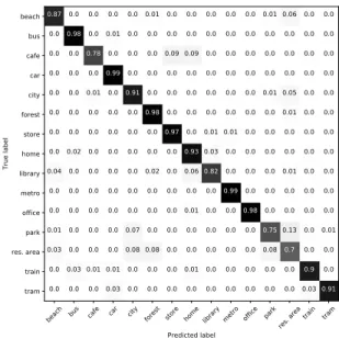
beach bus cafe car city forest store home library metro office parkres. areatrain tram Predicted label beach bus cafe car city forest store home library metro office park res. area train tram True label 0.87 0.0 0.0 0.0 0.0 0.01 0.0 0.0 0.0 0.0 0.0 0.01 0.06 0.0 0.0 0.0 0.98 0.0 0.01 0.0 0.0 0.0 0.0 0.0 0.0 0.0 0.0 0.0 0.0 0.0 0.0 0.0 0.78 0.0 0.0 0.0 0.09 0.09 0.0 0.0 0.0 0.0 0.0 0.0 0.0 0.0 0.0 0.0 0.99 0.0 0.0 0.0 0.0 0.0 0.0 0.0 0.0 0.0 0.0 0.0 0.0 0.0 0.01 0.0 0.91 0.0 0.0 0.0 0.0 0.0 0.0 0.01 0.05 0.0 0.0 0.0 0.0 0.0 0.0 0.0 0.98 0.0 0.0 0.0 0.0 0.0 0.0 0.01 0.0 0.0 0.0 0.0 0.0 0.0 0.0 0.0 0.97 0.0 0.01 0.01 0.0 0.0 0.0 0.0 0.0 0.0 0.02 0.0 0.0 0.0 0.0 0.0 0.930.03 0.0 0.0 0.0 0.0 0.0 0.0 0.04 0.0 0.0 0.0 0.0 0.02 0.0 0.060.82 0.0 0.0 0.0 0.01 0.0 0.0 0.0 0.0 0.0 0.0 0.0 0.0 0.0 0.0 0.0 0.99 0.0 0.0 0.0 0.0 0.0 0.0 0.0 0.0 0.0 0.0 0.0 0.0 0.01 0.0 0.0 0.98 0.0 0.0 0.0 0.0 0.01 0.0 0.0 0.0 0.07 0.0 0.0 0.0 0.0 0.0 0.0 0.750.13 0.0 0.01 0.03 0.0 0.0 0.0 0.08 0.08 0.0 0.0 0.0 0.0 0.0 0.08 0.7 0.0 0.0 0.0 0.03 0.01 0.01 0.0 0.0 0.0 0.01 0.0 0.0 0.0 0.0 0.0 0.9 0.0 0.0 0.0 0.0 0.03 0.0 0.0 0.0 0.0 0.0 0.0 0.0 0.0 0.0 0.030.91
Figure 2: Normalized confusion matrix for the system fusion.
and the `1 and `2 regularization terms to λ1 = 0.2 and λ2 = 0.
After preliminary experiments, the gradient step is set to ρ = 0.001 for the original algorithm [11] and to ρ = 0.0005 for the modified algorithm presented in Section 2.2. We follow the same decaying strategy as described in [19]. Moreover, contrary to our previous application of TNMF [8], we classify each slice individually and average the log-probabilities to take a decision on the full examples. The performance of our adapted scaling algorithm is compared to the previously used TNMF algorithm for ASC in the first part of Table 1. The results are shown for different values of dictionary size K and are averaged over 10 initializations of the model. As a baseline we also include the results for an unsupervised NMF-based feature learning system classified with logistic regression. For both dictionary sizes, the proposed modifications for the algorithm al-low for a notable increase in performance. This confirms that the introduced adaptive scaling strategy in the algorithm improves the model generalization capacity. Moreover the proposed TNMF sys-tem largely outperforms the dataset baseline as well as the unsuper-vised NMF-based systems.
4.4. Comparing DNN architectures
When used to train DNNS, the unsupervised NMF features are
ex-tracted using the Kullback-Leibler divergence with a `1 sparsity
constraint λ1= 0.2. The DNNs are trained separately on the NMF
activations or the time-frequency representation, we keep the same DNN architectures as proposed in our previous work on the same dataset [17]. The networks have 2 hidden layers of 256 units when having NMF features as an input and 3 hidden layers with 512 units when trained on the CQT representations. All layers have recti-fied linear unit (ReLU) [25] activations and dropout probability of 0.2 [26]. The models are trained with keras [27] using the stochastic gradient descent algorithm with default settings on 50 epochs with-out early stopping. The architecture of the merged CQT-NMF DNN model is described in Figure 2 and is trained with the same settings as just described.
The results of the compared DNN systems are reported in the second part of Table 2. First, as it was found in [17], training DNN directly on the NMF largely outperforms those trained directly on time-frequency representation as well as unsupervised NMF trained with a logistic regression. The proposed merged DNN architecture helps slightly increasing the performance compared to DNN trained only on NMF activations. Moreover it allows us to reach accuracies similar to the best TNMF system. However, as the networks are trained from unsupervised NMF features they require more compo-nents to attain the best results. We can also note that the TNMF-AS model still provides better results compared to the best DNN-M model which further confirms its usefulness for the task.
4.5. Fusion for final system
In order to further improve the results of our final system we aug-ment the data by using both channels of the stereo signal instead of the mono mix used previously and apply late fusion to combine the output of the systems described above. The systems trained on both channels will be denoted as ”TNMF-AS stereo” and ”DNN-M stereo” and are reported in the fourth part of Table 2. The results are averaged over 10 different initializations of the models. Our fi-nal system fusion is computed with the following process similar to the one proposed in [11]:
• Train 4 initializations DNN-M-Stereo for K = 1024 on the 4 training sets and store the resulting 16 output log-probabilities • Train 4 initializations TNMF-AS stereo K = 512 on the 4 training sets and store the resulting 16 output log-probabilities • Average all log-probabilities in order to make the final
predic-tions
The log-probabilities of the models trained on each of the 4 avail-able training sets in the development set. We also report and sub-mitted the system using only the log-probabilities computed with TNMF-AS which is denoted as TNMF-AS fusion. The accuracy obtained for the separate systems with both channels and the fusion systems are reported in the last row of Table 1. The accuracy scores on the development set go from 88.4 and 89.2% for TNMF-AS and DNN-M systems respectively to 90.1% with the fusion of both sys-tems. The normalized confusion matrix for the last fusion system is shown in Figure 2. The majority of confusions comes from labels corresponding to similar scenes such as park and residential area,
library and officeor restaurant and grocery store. In fact, such
pairs of acoustic environments tend to contain many event queues in common that could make it difficult for the systems to discrimi-nate between them.
5. CONCLUSION
In this paper we have described the system we submitted to the 2017 DCASE challenge for acoustic scene classification. We use two es-tablished methods to learn nonnegative representations of acoustic scenes, a supervised NMF method and DNN trained on unsuper-vised NMF activation features. Moreover, we propose improve-ments to both methods in order to improve classification perfor-mance. We introduce a new adaptive scaling algorithm for TNMF and DNN architecture that learns from both the time-frequency rep-resentation and the NMF features. Finally we use a fusion of both methods as our final system. For future work, we could investigate in what respect NMF representation can be jointly learned with the networks in the TNMF.
6. REFERENCES
[1] D. Barchiesi, D. Giannoulis, D. Stowel, and M. D. Plumbley, “Acoustic scene classification: Classifying environments from the sounds they produce,” IEEE Signal Processing Magazine, vol. 32, no. 3, pp. 16–34, 2015.
[2] A. Mesaros, T. Heittola, and T. Virtanen, “Tut database for acoustic scene classification and sound event detection,” in Proc. of European Signal Processing Conference, 2016. [3] A. J. Eronen, V. T. Peltonen, J. T. Tuomi, A. P. Klapuri,
S. Fagerlund, T. Sorsa, G. Lorho, and J. Huopaniemi, “Audio-based context recognition,” IEEE Transactions on Audio, Speech, and Language Processing, vol. 14, no. 1, pp. 321– 329, 2006.
[4] X. Valero and F. Al´ıas, “Gammatone cepstral coefficients: bi-ologically inspired features for non-speech audio classifica-tion,” IEEE Transactions on Multimedia, vol. 14, no. 6, pp. 1684–1689, 2012.
[5] G. Roma, W. Nogueira, and P. Herrera, “Recurrence quantifi-cation analysis features for environmental sound recognition,” in Applications of Signal Processing to Audio and Acoustics (WASPAA), 2013.
[6] A. Rakotomamonjy and G. Gasso, “Histogram of gradients of time-frequency representations for audio scene classifica-tion,” IEEE/ACM Transactions on Audio, Speech and Lan-guage Processing (TASLP), vol. 23, no. 1, pp. 142–153, 2015. [7] D. Battaglino, L. Lepauloux, L. Pilati, and N. Evansi, “Acous-tic context recognition using local binary pattern codebooks,” Proc. Workshop on Applications of Signal Processing to Audio and Acoustics, pp. 1–5, 2015.
[8] V. Bisot, R. Serizel, S. Essid, and G. Richard, “Feature learn-ing with matrix factorization applied to acoustic scene classifi-cation,” IEEE/ACM Transactions on Audio, Speech, and Lan-guage Processing, vol. 25, no. 6, pp. 1216–1229, June 2017. [9] J. Salamon and J. P. Bello, “Unsupervised feature learning for
urban sound classification,” in Proc. of International Confer-ence on Acoustics, Speech and Signal Processing (ICASSP). IEEE, 2015.
[10] A. Rakotomamonjy, “Supervised representation learning for audio scene classification,” IEEE/ACM Transactions on Au-dio, Speech, and Language Processing, vol. 25, no. 6, pp. 1253–1265, 2017.
[11] V. Bisot, R. Serizel, S. Essid, and G. Richard, “Supervised nonnegative matrix factorization for acoustic scene classifica-tion,” DCASE2016 Challenge, Tech. Rep., September 2016. [12] J. Li, W. Dai, F. Metze, S. Qu, and S. Das, “A comparison
of deep learning methods for environmental sound,” arXiv preprint arXiv:1703.06902, 2017.
[13] M. Valenti, A. Diment, G. Parascandolo, S. Squartini, and T. Virtanen, “DCASE 2016 acoustic scene classification us-ing convolutional neural networks,” DCASE2016 Challenge, Tech. Rep., 2016.
[14] H. Eghbal-Zadeh, B. Lehner, M. Dorfer, and G. Widmer, “CP-JKU submissions for DCASE-2016: a hybrid approach using binaural i-vectors and deep convolutional neural networks,” DCASE2016 Challenge, Tech. Rep., September 2016.
[15] H. Phan, P. Koch, F. Katzberg, M. Maass, R. Mazur, and A. Mertins, “Audio scene classification with deep recurrent neural networks,” arXiv preprint arXiv:1703.04770, 2017. [16] A. Mesaros, T. Heittola, A. Diment, B. Elizalde, A. Shah,
E. Vincent, B. Raj, and T. Virtanen, “DCASE 2017 challenge setup: Tasks, datasets and baseline system,” in Proceedings of the Detection and Classification of Acoustic Scenes and Events 2017 Workshop (DCASE2017), November 2017, sub-mitted.
[17] V.Bisot, R. Serizel, S. Essid, and G. Richard, “Leveraging deep neural networks with nonnegative representations for im-proved environmental sound classification,” in Proc. of Work-shop on Machine Learning for Signal Processing, 2017. [18] D. D. Lee and H. S. Seung, “Learning the parts of objects by
non-negative matrix factorization,” Nature, vol. 401, no. 6755, pp. 788–791, 1999.
[19] J. Mairal, F. Bach, and J. Ponce, “Task-driven dictionary learning,” IEEE Transactions on Pattern Analysis and Ma-chine Intelligence, vol. 34, no. 4, pp. 791–804, 2012. [20] P. Sprechmann, A. M. Bronstein, and G. Sapiro, “Supervised
non-euclidean sparse nmf via bilevel optimization with appli-cations to speech enhancement,” in Proc. of Joint Workshop on Hands-free Speech Communication and Microphone
Ar-rays (HSCMA). IEEE, 2014, pp. 11–15.
[21] S. Ioffe and C. Szegedy, “Batch normalization: Accelerating deep network training by reducing internal covariate shift,” in International Conference on Machine Learning, 2015, pp. 448–456.
[22] B. Mathieu, S. Essid, T. Fillon, J. Prado, and G. Richard, “Yaafe, an easy to use and efficient audio feature extraction software.” in Proc. of International Society for Music Infor-mation Retrieval, 2010, pp. 441–446.
[23] R. Serizel, S. Essid, and G. Richard, “Mini-batch stochastic approaches for accelerated multiplicative updates in nonneg-ative matrix factorisation with beta-divergence,” in Machine Learning for Signal Processing (MLSP), 2016 IEEE 26th
In-ternational Workshop on. IEEE, 2016, pp. 1–6.
[24] F. Pedregosa, G. Varoquaux, A. Gramfort, V. Michel, B. Thirion, O. Grisel, M. Blondel, P. Prettenhofer, R. Weiss, V. Dubourg, et al., “Scikit-learn: Machine learning in python,” The Journal of Machine Learning Research, vol. 12, pp. 2825–2830, 2011.
[25] K. Jarrett, K. Kavukcuoglu, M. Ranzato, and Y. LeCun, “What is the best multi-stage architecture for object recognition?” in Proc. IEEE International Conference on Computer Vision, 2009, pp. 2146–2153.
[26] G. E. Hinton, N. Srivastava, A. Krizhevsky, I. Sutskever, and R. R. Salakhutdinov, “Improving neural networks by pre-venting co-adaptation of feature detectors,” arXiv preprint arXiv:1207.0580, 2012.