Distributed Simplicial Homology Based Load Balancing Algorithm for Cellular Networks

HAL Id: hal-01550198

https://hal.archives-ouvertes.fr/hal-01550198

Submitted on 1 Sep 2017

HAL is a multi-disciplinary open access

archive for the deposit and dissemination of

sci-entific research documents, whether they are

pub-lished or not. The documents may come from

teaching and research institutions in France or

abroad, or from public or private research centers.

L’archive ouverte pluridisciplinaire HAL, est

destinée au dépôt et à la diffusion de documents

scientifiques de niveau recherche, publiés ou non,

émanant des établissements d’enseignement et de

recherche français ou étrangers, des laboratoires

publics ou privés.

Distributed Simplicial Homology Based Load Balancing

Algorithm for Cellular Networks

Ngoc-Khuyen Le, Anaıs Vergne, Philippe Martins, Laurent Decreusefond

To cite this version:

Ngoc-Khuyen Le, Anaıs Vergne, Philippe Martins, Laurent Decreusefond. Distributed Simplicial

Homology Based Load Balancing Algorithm for Cellular Networks. IEEE 86th Vehicular Technology

Conference: VTC2017-Fall, Sep 2017, Toronto, Canada. �hal-01550198�

Distributed Simplicial Homology Based Load

Balancing Algorithm for Cellular Networks

Ngoc-Khuyen Le, Ana¨ıs Vergne, Philippe Martins and Laurent Decreusefond

Email: ngoc-khuyen.le, anais.vergne, philippe.martins, laurent.decreusefond@telecom-paristech.fr

Abstract—In this paper, we introduce a distributed load balancing algorithm for cellular networks. Traffic load in cellular networks is sometimes unbalanced. Some cells are overloaded, while others remain free. Simplicial homology is a tool from algebraic topology that allows to compute the coverage of a net-work by using only simple matrix computations. Our algorithm, which is based on simplicial homology, controls the transmission power of each cell in the network, not only to satisfy the coverage constraint, but also to redirect users from the overloaded cells to the underloaded ones. As a result, the traffic load of the cellular network is more balanced. The simulation results show that this algorithm improves the capacity of the whole network by 2.3% when the user demand is fast varying.

I. INTRODUCTION

Due to user mobility, some cells can be overloaded at some moments while the others are still underloaded at the same time. These underloaded cells have free resources that are not used. In other words, these free resources are wasted. In order to avoid this waste of resources, the traffic load in the network should be balanced for cells. However, cellular networks configurations are traditionally manual and costly as they lack a self-organized method to balance the traffic load between cells in real time.

There exists some load balancing methods. The first method is to borrow the bandwidth from low traffic cells, and give it to overloaded cells. Some bandwidth borrowing algorithms can be found in [12], [15], [16], [26]. However, the bandwidth borrowing may increase interference in the network. When the network is dense and the cell size is small, the interference is becoming hard and degrades strongly the quality of service.

Another method is to force the users to redirect from the overloaded cell to one of its neighbors that is underloaded. It can be done by modifying the hysteresis margin in the handover scheme between the overloaded cells and the un-derloaded cells, for example in [5], [20]. For more details about the handover scheme and the hysteresis margin, see [1]. Users can be also redirected from the overloaded cells to the underloaded cells by modifying the pilot power of cells. In [6], the underloaded cells attract more users by increasing its pilot power. However, the power of data channels is not changed. Users can be also associated with the underloaded cells by a cooperated resource allocation such as in [17], [23]. However, overload often happens when many users are located in a cell while only a few users are located in another. These methods do not take into account the distance between the redirected users and their target cells. The target cell, which should be

a free cell, is one of the overloaded cell’s neighbors. Due to the long distance between the redirected users and the base station of their target cells, many redirected users may suffer from a bad connection. In addition, most resource allocation schemes prefer to give access to the users that have better connection [22], therefore, these redirected users can lose their connection. The load balancing should guarantee not only the free resources, but also the coverage for users.

Recently, in [10] authors change the power of antenna beams in the selected directions. The overloaded base stations reduce the antenna beam power in the direction where some users are in outage, while the underloaded base stations increase their beams power. Thanks to the handover process, the users in outage will connect to the underloaded base stations. However, this method requires the full access to the positions of users, which is not always available. In addition, modifying the power of antenna beams changes the shape of cells, but no method to verify the coverage is presented.

In recent researches, simplicial homology is often used to analyze the coverage of wireless networks. The wireless network is represented by a simplicial complex. Then, the information about the topology of the network is obtained via its homology. The ˇCech complex is the most suitable simplicial complex to represent the wireless network as it captures exactly its topology [8]. The construction of the

ˇ

Cech complex for the wireless network is introduced in [18]. Some applications based on simplicial homology have been proposed. In [14], [7], [9], [25], simplicial homology is used to detect coverage holes. In [24], it is used to turn off redundant cells. And in [19], it is used to save energy for wireless networks.

In this paper, we introduce a distributed load balancing algorithm for cellular networks, which not only solves the overload problem for the base stations but also ensures a strong quality of service for every user. Our algorithm changes the transmission power for each base station in order to redirect some users in the overloaded cells to the underloaded ones via the handover process. Then, the traffic loads in different cells are balanced. We use the simplicial ˇCech complex [18] to represent the topology of the network. Thanks to simplicial homology theory, the coverage of the network is always computable. This allows us to always ensure the coverage of the network as well as to avoid the interference due to the redundant transmission power. In addition, our algorithm increases the transmission power of the cells that have enough

free resources to allocate to the redirected users. Furthermore, our algorithm does not need any information about the posi-tions of users.

The remainder of this paper is organized as follows. Sec-tion II introduces basic noSec-tion about simplicial homology and its applications. Section III is devoted to describe all the details about our load balancing algorithm. The simulation results will be presented in Section IV. Finally, we conclude and discuss our works in Section V.

II. SIMPLICIAL HOMOLOGY

In this section, we introduce some notions of algebraic topology. We also explain how these tools can be used to capture and analyze the topology of the network. For more details about algebraic topology, see [21].

A. Simplicial complex

Let Sk = {v0, v1, . . . , vk} be a geometrically independent set of k + 1 points in Rn_{, where n > k. The convex hull} of S is called a k-simplex, denoted sk. The number k is its dimension and v0, v1, . . . , vk are its vertices. Thus, a single point is a 0-simplex, an edge is an 1-simplex, a triangle is a 2-simplex, a tetrahedron is a 3-simplex, and on and on. See Figure 1 for some instances.

v0 0_{-simplex 1-simplex} v0 v1 2_-simplex v0 v1 v2 3_-simplex v0 v1 v2 v3

Fig. 1: An example of simplices.

Any subset ofSk is also geometrically independent, there-fore the convex hull of this subset is a simplex of a lower dimension. Letl be the dimension of this simplex, this simplex is called a l-face of sk. An abstract simplicial complex is a collection of simplices such that: every face of a simplex is also in this collection.

B. Homology group

The orientation of a simplex is determined by an ordering of its vertices. A simplex {v0, v1, . . . , vk} together with an ordering of its vertices is denoted as [vo, v1, . . . , vk]. The orientation of a simplex changes into the inverse one if the ordering of its vertices is transformed by an odd permutation. In instance, if two vertices of a simplex are swapped, then the orientation of this simplex changes to the opposite one, denoted by the negative sign as:

[v0, . . . , vi, . . . , vj, . . . , vk] = −[v0, . . . , vj, . . . , vi, . . . , vk]. Let us denote K an abstract simplicial complex, we can define for each k the k-chain group Ck(K) as the vector space spanned by the set of oriented k-simplices of K. Let [v0, v1, . . . , vk] be a k-simplex, which is viewed as a basic element ofCk. The boundary map ∂k is defined as the linear transformation ∂k : Ck(K) → Ck−1(K) which acts on basis elements via: ∂k[v0, v1, . . . , vk] = k X i=0 (−1)i[v0, v1, . . . , vi−1, vi+1, . . . , vk], where[v0, v1, . . . , vi−1, vi+1, . . . , vk] is the i-th face obtained by deleting the i-th vertex. This formula tells us that the boundary of a k-simplex is its collection of (k − 1)-faces. A simple computation shows that∂k◦ ∂k+1= 0, this means that the boundary of a chain has no boundary. We call a k-chain a k-cycle if its boundary is zero. So, the group of k-cycles, denoted asZk(K), is the kernel of ∂k: Ck(K) → Ck−1(K). Let Bk(K) be the group of k-boundaries, it is the image

of ∂k+1 : Ck+1(K) → Ck(K). Since ∂k ◦ ∂k+1 = 0 for

each k, it implies that every k-boundary is also a k-cycle. It follows that Bk(K) ⊂ Zk(K) for all k. We can now define the k-th homology group of K as the quotient vector space:

Hk(K) = Zk(K)/Bk(K). The dimension of k-th homology

group is called the k-th Betti number:

βk = dim Hk = dim Zk− dim Bk. (1)

This number has an important meaning in solving coverage problems. Given a simplicial complex that captures the topol-ogy of a network, its k-th Betti number βk counts the k-dimensional holes. For example, the β0 counts the connected components while theβ1counts the coverage holes. Therefore, the network is connected ifβ0= 1, and there is no coverage hole ifβ1= 0.

C. Simplicial complex of cellular networks

Definition 1 ( ˇCech complex): Given a collection of cover

sets U, the ˇCech complex of U, denoted as ˇC(U), is the abstract simplicial complex whosek-simplices correspond to nonempty intersection of k + 1 distinct elements of U.

If each cover set in the collectionU is a disc that presents the coverage of a cellular cell, then the ˇCech complex of U captures exactly the topology of the network [18].

Fig. 2: Cells and their ˇCech representation.

For example, in Figure 2, the overlapping region of coverage of four cells 0, 1, 2 and 6 is represented by a tetrahedron, which is a 3-simplex. The overlapping region of coverage of three cells 2, 3 and 6 is represented by a triangle, which is a 2-simplex. The coverage hole inside four cells 3, 4, 5 and 6 is represented by an empty space that is bounded by four edges 3-4, 4-5, 5-6 and 6-3, which are a chain of 1-simplices. The numberβ0= 1 indicates that all cells are connected. The numberβ1= 1 indicates that there is a coverage hole.

III. DISTRIBUTED LOAD BALANCING ALGORITHM

In this section, we entirely describe the details about our load balancing algorithm. We are considering a cellular network with high traffic. We assume that the coverage of the network is satisfied before performing the load balancing algorithm. This means that before applying our load balancing

algorithm, there is no coverage hole in the network. We consider a cellular network that contains a collection of cells: C = {ci(vi, ri) | i = 1, 2, . . . , N }, where N is the number of cells, and ci(vi, ri) is the i-th cell centered at the position of its base station vi and covering the space within a radiusri.

Let pt,i be the transmission power of the cell ci and u be a user in this cell. The distance from the user u to the base station ci is du,i. The path loss from the base station ci to the position of the user u is Li,u(du,i). To estimate the path loss Li,u(du,i), we use the COST-231 model [4]. Let ps be the sensitivity of the mobile device, the coverage radius ri of the i-th cell ci is the maximum distance du,i that satisfies pt,i−Li(du,i) ≥ ps. So, the radiusriof the cellciis controlled by the transmission powerpt,i.

Each base station ci periodically computes the requested traffic load, denoted ρi, which is generated by its registered

users as: ρi = P

k

ρi,k/µi, where ρi,k is the number of requested resource blocks of the k-th registered user and µi is the capacity of the base station ci. The capacity of a base station is the total number of resource blocks that are available in this base station. Each resource block is a group of 12 consecutive subcarriers, where each subcarrier has a bandwidth of 15kHz. For the details about the resource blocks, see [2]. A base station is called hot, or overloaded if its requested traffic load is greater than one. It is called warm if it is not hot and its requested traffic load is greater than a warm load threshold ρwsuch that0 < ρw< 1. Otherwise, the base station is called cool, or underloaded.

We assume that all cells are connected by the backhaul network. Each cell ci can transmit information about its position and its coverage radius to every cell via this backhaul network. We also assume that the cells can cooperate to cancel the interference in the overlapping regions [13]. Therefore, the cells can adjust their transmission power without the interference problem. We say that two cells are neighbors if the coverage of each one intersects with the coverage of the other. Then, each cell ci can compute its table of neighbors Ni and sends its requested traffic load ρi to its neighbors in Ni. Therefore, each base station knows information about the requested traffic load, the position and the coverage of itself and of all its neighbors.

If the base station ci is hot, then it needs to reduce its requested traffic load. One solution is to redirect some of its currently registered users to its neighbors via handovers. Han-dovers would happen automatically when a cool neighbor cell increases its coverage radius, while a hot cell decreases one. In order to do that, a hot cell chooses a neighbor cell which has a lot of free resource blocks, i.e. a cool cell and requests it to help. The neighbor that is chosen is called a helper. A neighbor that is warm can not be chosen to be a helper. This will prevent a helper from becoming hot after having received the redirected users from the hot base station. The helper of the cell ci is defined as the neighbor ch that has the lowest traffic load: ch = arg min

cj∈Ni

ρj such thatρj ≤ ρw. If there is no available helper, the cell ci redoes the process in the

next time frame. To attract users via handover, helper cells not only need free resource blocks but also a stronger signal. However, the redirected users in outage that are currently in the hot cellcican be outside the coverage of the helperch. The helperchneeds to increase its transmission power by a power step ∆ph. At the same time, the helper ch transmits its new coverage radius to other cells. It also requests its neighbors to reduce their transmission power if possible. However, a fast reduction of transmission power may create a coverage hole. Each neighbor of the helper ch, denoted ck, computes the coverage with a transmission power decreased by∆pk/2, where∆pk is the power step of the cell ck. If this reduction does not create any coverage hole, the base stationck reduces its transmission power by∆pk/2 and sends its new coverage radius to other cells. If a coverage hole appears, this cell must keep its transmission power as the original value. If a neighbor is the helper of another cell, it will ignore the request to reduce transmission power. To verify if a coverage hole appears, the shrunk cell constructs a ˇCech complex for a local region that includes itself and its neighbors. For the details about the construction of the ˇCech complex, we refer to [18]. Then the information about the coverage can be tractable through the computation of Betti numbers (1) of this ˇCech complex. If no coverage hole appears after the reduction, the Betti numbers

must be β0 = 1 and β1 = 0. Otherwise, a coverage hole

appears. To verify the coverage of the network, we need to compute only β0 and β1. Therefore, the ˇCech complex is only computed up to dimension two. The verification of the coverage of the network is summarized as in the Algorithm 1. Algorithm 1 Verification of coverage holes

Input: ci the shrunk cell and its neighbors setNi; Output: true ⇐⇒ a coverage hole appears;

compute ˇC_{= the ˇCech complex ofci∪ Ni;} computeβ0 andβ1 of ˇC; verification = false; ifβ06= 1 or β16= 0 then verification = true; end if return verification;

We should note that, a coverage hole may appear due to an outdated information about coverage radius. Therefore, whenever a cell tries to reduce its coverage radius, it firstly sends a “pause” signal to its neighbors. Then, it obtains the information from neighbors and processes the reduction. When it finishes the reduction, it sends a “continue” message to its neighbors to indicate them that they can continue. If a cell receives a “pause” signal, it pauses the balancing process and waits until a “continue” signal is received. To avoid an infinite wait in a special case that two neighbors send “pause” at the same time, and both of them receive the “pause”, if one cell sends the “pause” and receives another “pause” before it sends a “continue”, it waits in a random period of time then tries to send “pause” again.

Let us consider a special case where small cells are de-ployed, such as: pico and micro cells. The transmission power of macro cells is much higher than the one of small cells. If a small cell is hot, and it chooses a macro cell to be a helper, then it does not send a help request to the macro cell. The small cell directly reduces its transmission power if the verification of the coverage allows it as in the Algorithm 1, and broadcasts the new information to other cells. This prevents the unnecessary modification of macro cells transmission power that would affect many other small cells inside the macro cells.

Algorithm 2 Load balancing algorithm applied to each cellci Input: ci the i-th cell, and ρw the warm load threshold; Output: balanced traffic load for the cellci;

for each time frame do

send position and coverage radius to every cell; compute the requested traffic load ρi;

collect position and coverage radius of other cells; build the neighbors setNi ofci;

send requested traffic loadρi to neighbors inNi; collect requested traffic load of neighbors inNi; if ρi> 1 then

helper cell ch= arg min

cj∈Ni

ρj such thatρj < ρw; if ch6= null then

if ci is not macro cell andch is macro cell then obtain coverage radius of neighbors;

pt,i= pt,i− ∆pt,i/2;

if a coverage hole appears then pt,i= pt,i+ ∆pt,i/2; else

send new radius to every cell; end if

else

send request to increase power toch; end if

end if end if

if ci is the helper then pt,i= pt,i+ ∆pt,i;

send new radius to every cell;

send request to reduce the transmission power to neigh-bors of ci;

else

if ci received a reduce power request message then obtain information from neighbors;

pt,i= pt,i− ∆pt,i/2;

if a coverage hole appears then pt,i= pt,i+ ∆pt,i/2; else

send new radius to every cell; end if

end if end if end for return

The procedure to balance the traffic load for each base station, which is described in the Algorithm 2, is repeated in every radio time frame. In this procedure, the “pause” message is automatically sent before a base station tries to reduce its transmission power. Similarly, the “continue” message is also automatically sent after a reduction. In the description of this algorithm, we do not insert the “pause” and “continue” messages for a smooth reading.

In the load balancing algorithm, the requested traffic load can be computed in an instant, while the coverage verification is still needed for only the local region. We recall that the local region is comprised of the cell which reduces its coverage and its neighbors. This verification needs the computation of the

ˇ

Cech complex for this local region and its Betti numbersβ0, β1. In the worst case where every cell is neighbor of the others, the complexity of the ˇCech complex is stillO(N3_{), where N is} the number of cells in the network [18]. In this case, there are m1 = C2

N 1-simplices and at most m2= C 3

N 2-simplices in the ˇCech complex. Following [11], the complexity to compute β0 isO(m1), and the complexity to compute β1is equivalent to the computation time of the rank of a matrix that has m2 columns and m2 rows. The complexity to compute this rank by SVD method is O(m3_{2) [3]. Therefore, the complexity to} compute the ˇCech complex and its Betti numbers β0, β1 is O(N9_{), which is only polynomial time. As a result, the load} balancing algorithm has the complexity of polynomial time.

IV. SIMULATION RESULTS

A. Network deployment

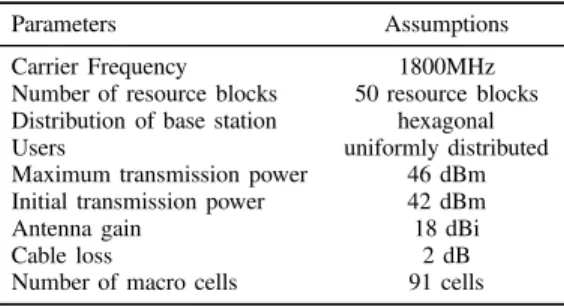
We deploy the macro cells according to the hexagonal model. In each macro cell, we deploy two micro cells, which are placed randomly following a uniform law in the coverage of macro cells. The parameters about the macro cells and the micro cells are summarized in Table I and Table II. However, micro cells are often deployed in the rear side of macro cells to increase the coverage at cell edge. In addition, if a micro cell is deployed too close to a macro cell’s base station, due to the much stronger signal from the base station of the macro cell, the users will connect to the macro cell even when they are very close to the micro cell’s base station. In our simulations, the macro cells and the micro cells are separated by a distance greater than two thirds of the macro cell coverage radius.

TABLE I: Macro cell parameters

Parameters Assumptions

Carrier Frequency 1800MHz Number of resource blocks 50 resource blocks Distribution of base station hexagonal Users uniformly distributed Maximum transmission power 46 dBm Initial transmission power 42 dBm

Antenna gain 18 dBi

Cable loss 2 dB

Number of macro cells 91 cells

We assume that the number of requested resource blocks of each user follows a Poisson law. In average, each user

TABLE II: Micro cell parameters

Parameters Assumptions

Carrier Frequency 1800MHz Number of resource blocks 15 resource blocks Distribution of base station uniformly distributed Users uniformly distributed Maximum transmission power 30 dBm Initial transmission power 24 dBm

Antenna gain 18 dBi

Cable loss 2 dB

Number of micro cells 182 cells

requests two resource blocks. We denoteRtotalthe total number of requested resource blocks, which is generated by all users in the network. And, we denote Ctotal the total capacity of all cells in the network, where the capacity of each cell is the total number of available resource blocks in this cell. The traffic load T of the network is: T = Rtotal/Ctotal. In our simulations, we analyze the performance of the algorithm with a given traffic load T . We generate the total number of requested resource blocksRtotalaccording to the Poisson point process of intensity T × Ctotal.

We assume that the total number of requested resource blocks in the micro cells and the macro cells are proportional to their capacity. The number of requested resource blocks in the micro cells is Rmicro = Rtotal× Cmicro

Cmico+Cmacro. We then

generate the users in the micro cells first. The users positions are uniformly distributed in coverage of all micro cells. The number of requested resource blocks of each user is generated following a Poisson law with intensity of two resource blocks. When the accumulated number of requested resource blocks in all micro cells reaches the number Rmicro, we stop the process of generating the users in the micro cells. Similarly, we generate the users in the macro cells until the total number of requested resource blocks in the network reachesRtotal.

We assume the COST-231 model for the radio propaga-tion [4] with the correcpropaga-tion c = 3 for urban areas. The sensitivity of the terminal is -104 dBm. The body loss at user mobile is 3 dB. The load balancing algorithm is performed for each cell in each time frame, which is assumed to be 10 ms. B. Performance with varying traffic load

In this subsection, we consider the performance of the load balancing algorithm when the users change their number of requested resource blocks frequently. We assume that each user changes its demand of resource blocks every 10 time frames. In each time frame, each cell applies the load balanc-ing algorithm one time.

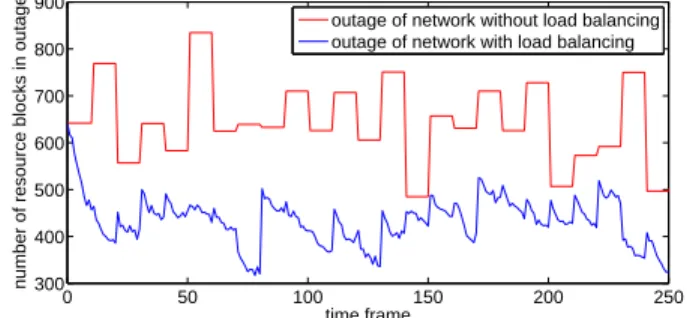
We assume that the average requested traffic load in the network is 0.9, it means the total number of requested resource blocks is 90% of the total capacity of the network in average. Although the average requested traffic load is less than one, the number of resource blocks demanded by each user is random. Some cells in network are overloaded while others are free. We define the outage of each cell as the number of requested resource blocks in this cell that are not serviced. The outage of the network is the accumulated outage of every cell.

In this simulation, the warm load threshold ρw is set to 0.9 and the power step ∆p is set to 1dB for every cell. We perform the simulation in 250 time frames and record the outage of network in two cases: without load balancing applied and with load balancing applied. We show one example of simulation in Figure 3. The outage of system in the case that the load balancing is not applied is drawn as the red line. The outage of system in the case that the load balancing is applied is drawn as the blue line. Because the users change their demand of resource blocks every 10 time frames, the outage of system when the load balancing is not applied is also changed every 10 time frames. The blue line is under the red line, this shows that by using the load balancing, the outage of system is reduced. The number of reduced resource blocks in outage is the capacity gain of system. In the Figure 3, the difference between the red line and the blue line describes the capacity gain of the load balancing algorithm. The simulation is repeated 1000 times. In average, this load balancing algorithm reduces the number of resource blocks in outage by 25.7%, and gains 2.3% of the capacity of the whole system. 0 50 100 150 200 250 300 400 500 600 700 800 900 time frame

number of resource blocks in outage

outage of network without load balancing outage of network with load balancing

Fig. 3: An instance of total outage of a varying traffic network with and without load balancing on the same scenario: base stations, users positions and user requests are identical in both cases.

C. Performance with constant traffic load

In this subsection, we consider the performance of the load balancing algorithm when the traffic load is kept constant. Indeed, the demand of resource blocks of each user is un-changed during the simulation. Some properties of the load balancing algorithm such as: capacity gain, convergence speed and stability are considered at different requested traffic load T of the network from the low one to the high one. When the requested traffic load of the network is low, it is also necessary to analyze the performance of the load balancing algorithm. Due to the mobility of users, some cells may be overloaded while others are not.

The total requested traffic load of networkT varies from 0.5 (low) to 0.9 (high). We perform the load balancing algorithm with different values of warm load threshold ρw and power step ∆p. The simulation is performed in 200 time frames. Each time we change the value of one of these parameters, we repeat the simulation 100 times. The warm load threshold ρw and the power step ∆p are assumed to be the same for every cell.

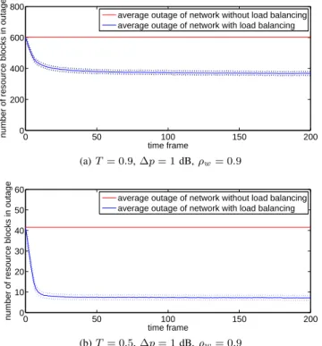
First, we consider the performance of the load balancing

algorithm when the network is high loaded T = 0.9 in

Figure 4a and when the network is low loaded T = 0.5 in Figure 4b. The warm load threshold ρw is set to 0.9 and the power step ∆p is 1 dB for all cell. The users do not change their demand of resource blocks in each simulation, then the outage of network when the load balancing is not applied is the same in every time frame and is drawn by a red line. The blue line draws the average outage of network when the load balancing is applied. The dotted line shows the upper bound and lower bound of the 95% confidence interval of the average outage of the balanced network. The outage of the balanced network is quickly reduced. When T = 0.9, the outage of the network is reduced by 34% within 28 time frames. When T = 0.5, the outage of the network is reduced by 80% during 16 time frames. 0 50 100 150 200 0 200 400 600 800 time frame

number of resource blocks in outage

average outage of network without load balancing average outage of network with load balancing

(a) T = 0.9, ∆p = 1 dB, ρw= 0.9 0 50 100 150 200 0 10 20 30 40 50 60 time frame

number of resource blocks in outage

average outage of network without load balancing average outage of network with load balancing

(b) T = 0.5, ∆p = 1 dB, ρw= 0.9

Fig. 4: Average outage of the constant traffic load network We should note again that the number of reduced requested resource blocks in outage is the capacity gain of the network. The capacity gain is recorded at the last time frame of simulation, the 200-th time frame. The Figure 5a compare the capacity gain of network at different requested traffic loads T when the load balancing is applied with different warm load thresholdsρw. The power step∆p is set to 1 dB. When the requested traffic load of the network is high, the higher warm load threshold ρw is, the higher capacity gain is. In Figure 5b, the capacity gain is compared when the load balancing is applied with different power steps ∆p = 1 dB and∆p = 0.25 dB. The warm load threshold ρwis set to 0.9. At each requested traffic load T , the capacity gains in long term with different power steps∆p are almost equal.

0.5 0.6 0.7 0.8 0.9 0 1 2 3 4

Total traffic load of network

Capacity gain (%)

warm load threshold ρw = 0.60 warm load threshold ρ

w = 0.75 warm load threshold ρw = 0.90

(a) different ρwand ∆p = 1 dB

0.5 0.6 0.75 0.8 0.9 0 1 2 3 4

Total traffic load of network

Capacity gain (%)

power step ∆p = 0.25 dB power step ∆p = 1.00 dB

(b) different ∆p and ρw= 0.9

Fig. 5: Capacity gain of system

The different values of the warm load thresholdρwand the power step∆p may also affect other properties of performance such as: convergence speed and stability. We consider that the outage of the balanced network approaches the stability value within the first 100 time frames. Then, we compute the mean value of the outage of balanced network in the last 100 time frames. We denote this mean byM . When the outage of the balanced network goes below the value1.05 × M , we say the network converged at the current time frame t. The duration from starting point to this current time framet is defined as the convergence time of the network.

The convergence time is shown in Figure 6a with different warm load thresholds ρw, and in Figure 6b with different power steps∆p. With higher warm load threshold ρw, there are more available helpers, so more requests to help can be satisfied. Therefore, the process of requests and helps are longer. As a result, the convergence time is higher. The convergence time increases if the power step ∆p is reduced. A significant increase of convergence time is shown when the power step is reduced in Figure 6b. As shown in Figure 5b, the capacity gains with different power steps ∆p are almost the same. This shows that a smaller ∆p reduces the speed of convergence but does not change the capacity gain in long term. In varying traffic load network, we should not choose a so small power step ∆p because of the slow convergence speed. 0.5 0.6 0.7 0.8 0.9 0 10 20 30 40 50 60

Total traffic load of network

Number of time frames

warm load threshold ρ_w = 0.60 warm load threshold ρ_w = 0.75 warm load threshold ρ_w = 0.90

(a) different ρw and ∆p = 1 dB

0.5 0.6 0.7 0.8 0.9 0 20 40 60 80

Total traffic load of network

Number of time frames

power step ∆p = 1.00 power step ∆p = 0.25

(b) different ∆p and ρw= 0.9

Fig. 6: Convergence time

We use the standard deviation of the outage of the balanced

network from the mean value M , denoted as σ, as the

measurement for the stability of the network. The Figure 7a and Figure 7b show values of σ with different ρw and ∆p. The higher warm load threshold is, the lower stability of the system is. In addition, reducing the power step can increase a little the stability of the system.

0.5 0.6 0.7 0.8 0.9 0 2 4 6 8 10 12

Total traffic load of network

Number of resource blocks

warm load threshold ρ_w = 0.60 warm load threshold ρ_w = 0.75 warm load threshold ρ_w = 0.90

(a) different ρwand ∆p = 1 dB

0.5 0.6 0.7 0.8 0.9 0 2 4 6 8 10 12

Total traffic load of network

Number of resource blocks

power step ∆p = 1.00 dB power step ∆p = 0.25 dB

(b) different ∆p and ρw= 0.9

Fig. 7: Standard deviation of the outage of balanced network V. CONCLUSION ANDDISCUSSION

In this paper, we introduce a distributed load balancing algo-rithm for self organized cellular networks. This algoalgo-rithm does not need information about the position of users, nor to modify the handover process. Our algorithm provides sufficient power and resources to allocate to users, and also guarantees the coverage of the network. This algorithm improves by 2.3% the capacity of the whole network when the user demand is varying very fast.

The simulations show that the value of the warm load threshold ρw and the power step ∆p should be carefully selected for each cell to keep the best performance and stability for the network. The higher value of the warm load threshold ρw gives the higher capacity gain. However, it makes the network less stable. In contrast, the lower value ofρwincreases the convergence speed and stability of the network, but it gives the lower capacity gain. The power step ∆p should be much smaller than the transmission power of the base station. However, a too small value of ∆p reduces the convergence speed of the network and therefore reduces the capacity gain of the load balancing algorithm when the traffic load requested by users are fast varying.

REFERENCES [1] 3GPP TS 36.300 V13.2.0 (2015-12).

[2] LTE Resource Guide. http://web.cecs.pdx.edu/∼fli/class/LTE Reource Guide.pdf. (accessed 10/04/2016).

[3] Singular value decomposition. https://en.wikipedia.org/wiki/Singular value decomposition. (accessed 20/04/2016).

[4] COST Action 231. Digital mobile radio towards future generation systems COST-231 final report.

[5] Heejung Byun and Junglok Yu. Automatic handover control for distributed load balancing in mobile communication networks. Wirel.

Netw., 18(1):1–7, January 2012.

[6] R. Combes, Z. Altman, and E. Altman. Self-organization in wireless net-works: A flow-level perspective. In 2012 Proceedings IEEE INFOCOM, pages 2946–2950, March 2012.

[7] V. De Silva and R. Ghrist. Coordinate-free coverage in sensor networks with controlled boundaries via homology. Int. J. Rob. Res., 25(12):1205– 1222, December 2006.

[8] Vin de Silva, Robert Ghrist, and Abubakr Muhammad. Blind swarms for coverage in 2-D. In Proceedings of Robotics: Science and Systems, Cambridge, USA, June 2005.

[9] P. Dotko, R. Ghrist, M. Juda, and M. Mrozek. Distributed computation of coverage in sensor networks by homological methods. Appl. Algebra

Eng., Commun. Comput., 23(1):29–58, April 2012.

[10] Lin Du, J. Bigham, and L. Cuthbert. Towards intelligent geographic load balancing for mobile cellular networks. IEEE Transactions on Systems,

Man, and Cybernetics, Part C (Applications and Reviews), 33(4):480–

491, Nov 2003.

[11] H. Edelsbrunner and S. Parsa. On the computational complexity of betti numbers: Reductions from matrix rank. In Proceedings of the

Twenty-Fifth Annual ACM-SIAM Symposium on Discrete Algorithms, SODA

’14, pages 152–160. SIAM, 2014.

[12] J. S. Engel and M. M. Peritsky. Statistically-optimum dynamic server assignment in systems with interfering servers. In Decision and Control,

1972 and 11th Symposium on Adaptive Processes. Proceedings of the

1972 IEEE Conference on, pages 177–177, Dec 1972.

[13] D. Gesbert, S. Hanly, H. Huang, S. Shamai Shitz, O. Simeone, and W. Yu. Multi-cell mimo cooperative networks: A new look at interfer-ence. IEEE Journal on Selected Areas in Communications, 28(9):1380– 1408, December 2010.

[14] Robert Ghrist and Abubakr Muhammad. Coverage and hole-detection in sensor networks via homology. In Proceedings of the 4th International

Symposium on Information Processing in Sensor Networks, IPSN ’05,

Piscataway, NJ, USA, 2005. IEEE Press.

[15] H. Jiang and S. S. Rappaport. Cbwl: a new channel assignment and sharing method for cellular communication systems. IEEE Transactions

on Vehicular Technology, 43(2):313–322, May 1994.

[16] Hua Jiang and S. S. Rappaport. Prioritized channel borrowing without locking: a channel sharing strategy for cellular communications. In

Global Telecommunications Conference, 1993, including a Communica-tions Theory Mini-Conference. Technical Program Conference Record,

IEEE in Houston. GLOBECOM ’93., IEEE, pages 276–280 vol.1, Nov

1993.

[17] Hongseok Kim, Gustavo De Veciana, Xiangying Yang, and Muthaiah Venkatachalam. Distributed α-optimal user association and cell load balancing in wireless networks. IEEE/ACM Trans. Netw., 20(1):177– 190, February 2012.

[18] Ngoc-Khuyen Le, P. Martins, L. Decreusefond, and A. Vergne. Con-struction of the generalized czech complex. In Vehicular Technology

Conference (VTC Spring), 2015 IEEE 81st, pages 1–5, May 2015.

[19] Ngoc-Khuyen Le, P. Martins, L. Decreusefond, and A. Vergne. Simpli-cial homology based energy saving algorithms for wireless networks. In

Communication Workshop (ICCW), 2015 IEEE International Conference on, pages 166–172, June 2015.

[20] A. Lobinger, S. Stefanski, T. Jansen, and I. Balan. Load balancing in downlink lte self-optimizing networks. In Vehicular Technology

Conference (VTC 2010-Spring), 2010 IEEE 71st, pages 1–5, May 2010.

[21] James Munkres. Elements of algebraic topology. Perseus Books, 1984. [22] J. So, H. C. Jeon, and D. Ahn. Joint proportional fair scheduling for uplink and downlink in wireless networks. In Vehicular Technology

Conference (VTC Spring), 2011 IEEE 73rd, pages 1–4, May 2011.

[23] K. Son, S. Chong, and G. D. Veciana. Dynamic association for load balancing and interference avoidance in multi-cell networks. IEEE

Transactions on Wireless Communications, 8(7):3566–3576, July 2009.

[24] A. Vergne, L. Decreusefond, and P. Martins. Reduction algorithm for simplicial complexes. In INFOCOM, 2013 Proceedings IEEE, pages 475–479, April 2013.

[25] Feng Yan, P. Martins, and L. Decreusefond. Connectivity-based dis-tributed coverage hole detection in wireless sensor networks. In Global

Telecommunications Conference (GLOBECOM 2011), 2011 IEEE, pages

1–6, Dec 2011.

[26] Ming Zhang and T. S. P. Yum. Comparisons of channel-assignment strategies in cellular mobile telephone systems. IEEE Transactions on