• Aucun résultat trouvé

Detecting interference through graph reduction

N/A
N/A
Protected

Academic year: 2021

Partager "Detecting interference through graph reduction"

Copied!
9
0
0

Texte intégral

(1)

HAL Id: hal-02435522

https://hal.inria.fr/hal-02435522

Submitted on 10 Jan 2020

HAL is a multi-disciplinary open access

archive for the deposit and dissemination of

sci-entific research documents, whether they are

pub-lished or not. The documents may come from

teaching and research institutions in France or

abroad, or from public or private research centers.

L’archive ouverte pluridisciplinaire HAL, est

destinée au dépôt et à la diffusion de documents

scientifiques de niveau recherche, publiés ou non,

émanant des établissements d’enseignement et de

recherche français ou étrangers, des laboratoires

publics ou privés.

Detecting interference through graph reduction

Denis Roegel

To cite this version:

Denis Roegel. Detecting interference through graph reduction. [Research Report] Loria & Inria Grand

Est. 1997. �hal-02435522�

(2)

Detecting interference through graph reduction

Denis Roegel

CRIN, BP 239, 54506 Vandœuvre-l`

es-Nancy cedex, France

Abstract

Parallel programs which run in a shared-memory model have several threads that may interfere. There are constraints between the threads and these con-straints can be modelled by a net. We present TLA nets, which are interesting for the representation of concurrent executions. A reduction operation is de-fined on these nets, in order to detect interferences. These interferences can be eliminated by adding com-ponents such as delays to the net. TLA nets are a graphical tool to explore the constraints of parallel programming.

Keywords: graphs, nets, reduction, rewriting,

in-terferences, concurrency, threads, TLA.

1

Introduction

When parallel programs run in a shared-memory model, there are usually several threads and these threads can interfere, thereby producing unwanted side-effects. It is possible to describe the structure of a program segment by a graph whose edges represent the changes in the system, and such graphs will be useful for detecting interferences at early stages. An example of such a graph is given in figure 1.

In this graph, the wavy edges represent instruc-tions, whereas the dashed lines represent dependen-cies. The wavy edges are labelled by abstract rep-resentations of the instructions, namely TLA [3] ac-tions. The parallel branches represent independent actions. All these concepts and notations will be de-tailed in section 2.1.

First, the formalism of the nets will be precisely presented. Then it will be shown how a network can be reduced and how the reduction makes it possible to detect interferences between different threads.

Email: roegel@loria.fr. x′= x + 1 x′= x + y y′= y + 1 z′= 2∗ y y′= z + 1 t′= y y′= y2 ∧ (x > 0) ∧ (x′= y− x) ∧ (x ≤ 0)∧ (x= y + x) x′= x2 z v1 v2 v3 v4 v5 v6 v7 v8 v9

Figure 1: Example of a TNet

2

Nets of actions

The nets of TLA actions, the TNets (TLA Nets), are defined here. The presentation is purely syntactic, and the precise semantics is defined by the reduction operation (see section 3). First, an intuitive seman-tics is given.

TNets are graphs having vertices and edges. There are two kinds of vertices and several kinds of edges. Some edges are labelled by TLA actions, or more pre-cisely, by contextual TLA actions. The vertices rep-resent states of a system and the labelled edges are its transitions.

The nets of interest to us will be finite nets: the number of vertices and edges will be finite and the loops will themselves be finite: by that it is meant that there are only a finite number of loops in the construction of the net, and that each of these loops is traversed only a finite number of times during the execution. In section 3, a procedure to eliminate the nets which do not satisfy the constraint of a finite

(3)

loop execution (hence, nets which do not halt ) will be given.

Finally, all the considered TLA actions will be de-terministic, that is, they will actually be functional relations.

The structure of the TNets articulates around the following concepts: sequence, concurrency, alterna-tive, delay, synchronization, local variables.

The elements at our disposal to build a TNet make it possible to construct a great many networks. How-ever, only some of these networks are of interest to us.

2.1

Elements of a TNet

The building blocks of a TNet are 1) the edge valued by an action, that is, a relation between two consec-utive states, and 2) the edge representing a waiting state. A wavy edge represents an edge valued by an action, the waving being an image of the activity, or more precisely, of the fact that variables can change their values in the corresponding action: . For simplicity, an action will often be given as a short-hand in place of an edge valued by an action. Actions without primed variables, namely predicates, can be represented by straight edges: . In general, edges are labelled by an action as it is the case in figure 1.

Each vertex represents a set of local states. A local state is a valuation of a set of variables. A state can actually be regarded as a control point.

These states are not given in extenso, in that the values of the variables are not given explicitely. On the contrary, what defines the valuation of the vari-ables in a state is the way this state is reached. Other formalisms, in particular the very similar notation of Lamport (predicate/action diagrams [4]), associate predicates or assertions to the different control points. The presence of assertions corresponds to an oper-ational view, whereas its absence corresponds to a denotational view.

The edges corresponding to actions are directed and link two vertices of a TNet. Intuitively, this means that the action represented by the edge allows the passage from the first state to the second state.

Two vertices can be linked by more than one ac-tion. Two cases are distinguished:

• The first case is parallelism: a and b occur

simul-taneously. The superior vertex is of type “AND”.

a b

• The second case represents an alternative: Here,

at most one of the two actions, a or b, can oc-cur. It is possible that none of them is executed, when one considers a fragment of a net made up of two actions among three, for instance. The top vertex is of type “OR” represented by “□”. Hence, we always set ourselves in the case of a

deterministic choice.

a b

Delay and synchronization are indicated using sim-ple and double dashed arrows. They introduce an ordering constraint between two actions.

Some variables can be local to several actions. This fact is represented by surrounding the set of con-cerned actions by a dotted line labelled with the lo-cal variable (see figure 1). We add as a constraint that the intersection of two dotted areas is necessarily one of these areas, which forbids nets where actions bound by two different local variables overlap.

The graphs under consideration will always have a source and a sink. This is natural since these con-cepts correspond to the initial and final states of the execution of a function.

However, many nets obtained by a combination of the primitive elements will give rise to problems we will try to detect and solve in section 3.

2.2

Formalization

The concepts that have been described in the previ-ous section are formalized here.

Definition 1 (deterministic action) An action A(x , x′) is said to be deterministic if the relation

represented by A is functional, that is, if x′ is a function of x .

For instance, x′= x + 1 (x′ is the value of x in the next state) is deterministic, but x′+ y′ = x + y is not.

Definition 2 (set of actions) We assume Act to be a set of deterministic TLA actions. This set will not be defined formally.

(4)

Definition 3 (variables of an action) The set of variables of an action is the union of the set of used variables (unprimed) and the set of modified vari-ables (primed): Var (a) = U(a)∪ M(a).

x′is always included in M(a) even if x is not mod-ified. One can view M(a) as the set of variables

con-strained by a.

Definition 4 (set of variables) Let V be a set of variables such that ∀a ∈ Act, Var(a) ⊆ V.

Definition 5 (set of values) We assume a set of values Val.

We will see in section 3 that the environment of the net must be taken into account for the reduction of the nets. The interaction between a net and its environment is based on the interaction between an action and the environment. Henceforth, we will add to each action some requirements with respect to the environment. In return, this will allow us to deduce properties that the net will guarantee. This will be detailed later.

Definition 6 (contextual actions) Let CA = (Act× P(V)) ∪ {⟨⊥, ⊥⟩}; CA represents the set of

actions with a condition on the context; ⟨a, r⟩ ∈ CA if r is a set of variables which must not be modified by the environment. In general,⟨a, r⟩ = ⟨a, U(a)⟩ where

U(a) is the set of variables used in a.

Definition 7 (set of dependencies) D = {⊥, ! , , $} is the set of dependencies. The elements of D must be distinct from the elements of Act. ⊥ will represent the absence of any link between two vertices of a net. ! and will represent the delay and $ the synchronization.

The nets can now be defined:

Definition 8 (net) A GTNet is a tuple ⟨V , br, edge, loc⟩ where:

• V is a finite set of vertices;

• br : V → {·, } is the branching func-tion: br (s) =“·” if s is an “AND” vertex and br (s) =“” if it is an “OR” vertex.

• edge : V2→ (P(CA) ∪ D) is the “edge”

func-tion. edge(v1, v2) ∈ P(CA) if v1 and v2 are

connected by TLA actions. edge(v1, v2) ∈ D if

v1 and v2 are simply linked by dependencies, or

are not linked at all.

• loc : V → P(V × V × CA) is the function which associates to each variable a set of edges where this variable is local. The set of edges is {(v1, v2, ar )∈ V × V × CA/ar ∈ edge(v1, v2)}.

If loc(v1) and loc(v2) are the edges where v1

and v2 are local variables, then either loc(v1)

loc(v2) =∅, or loc(v1)⊆ loc(v2), or loc(v1)

loc(v2). This constraint may make it necessary

to rename some variables.

Definition 9 (source of a net) v is a source if v ∈ V and ∀u ∈ V : edge(u, v) ̸∈ P(CA).

Definition 10 (sink of a net) v is a sink if v ∈ V and∀u ∈ V : edge(v, u) ̸∈ P(CA).

Definition 11 A TNet is a GTNet with a unique source and a unique sink. The sink v is such that br (v ) =·.

Definition 12 (action escaping from a vertex) The action a is said to escape a vertex s if

∃r ∈ P(V) : ⟨a, r⟩ ∈

u∈V

edge(s, u)

2.3

Example of a formal

representa-tion of a net

Consider figure 1. This net has nine vertices denoted by v1, v2, . . . , v9. We have: • V = {v1, v2, v3, v4, v5, v6, v7, v8, v9}. • ∀i ̸= 5 : br(vi) =· and br(v5) =□. • edges: edge(v1, v2) = {⟨x′ = x + 1,{x}⟩}, edge(v2, v3) = , edge(v5, v7) = {⟨(x > 0) ∧ (x′ = y − x), {x, y}⟩, ⟨(x ≤ 0) ∧ (x′ = y + x ),{x, y}⟩}, etc.

• loc(z) = {(v3, v4,⟨z′= 2∗ y, {y}⟩), (v4, v6,⟨y′=

z + 1,{z}⟩)}

• v1 is the source and v9is the sink.

3

Reduction of a net

A TNet reduction will replace a complex net by a net composed of a unique edge which is equivalent to it (in some sense). In other words, the reduction associates a TLA action to a net. This operation modifies the granularity of a net.

(5)

Moreover, the reduction makes it possible to sepa-rate the nets into two categories: those that can be reduced into an action and those that cannot. The case of nonreducible nets will be studied in more de-tail.

Underspecified nets have also to be completed. For instance

x′= x + 1

y′ = x + z

poses problems because it is not known how the value of z changes. The solution is twofold:

• All unprimed variables1 in the second action

must appear in the first action, in their primed form, possibly meaning the identity.

• If an action uses a variable x, it must also men-tion x′.

If these conditions are not respected, the reduction of these two actions is unknown by convention, and is denoted by⊥.

These rules will be formalized in the next section.

3.1

Formalization

The previous section explained intuitively how the net reduction is worked out, and the need to intro-duce additional constraints if we want the net to be reduced in a specific way.

From now on, TLA actions will no longer be ma-nipulated. Instead, contextual actions (cf. §2.2) are used in order to handle these constraints.

The operations ∧c, ∨c and •c are defined on the

elements of CA, the set of contextual actions. They are the contextual equivalents of∧, ∨ and •.

Definition 13 (contextual conjunction) ⟨a1, r1⟩ ∧c⟨a2, r2⟩ is defined as follows:

• if a1=⊥ or a2=⊥, then ⟨a1, r1⟩∧c⟨a2, r2 ∆ =

⟨⊥, ⊥⟩ (failure propagation)

• if M(a1)∩ r2 = ∅ and M(a2)∩ r1 = ∅, then

⟨a1, r1⟩ ∧c⟨a2, r2

= ⟨a1∧ a2, r1∪ r2

• otherwise, ⟨a1, r1⟩ ∧c⟨a2, r2

= ⟨⊥, ⊥⟩

1These variables can also occur as primed variables in the second action, of course.

As soon as a reduction yields⟨⊥, ⊥⟩, the reduction of the whole TNet is undefined. The result of the ex-ecution is ignored: the TNet must be better specified.

Definition 14 (contextual disjunction) ⟨a1, r1⟩ ∨c⟨a2, r2⟩ is defined as follows:

• if a1=⊥ or a2=⊥, then ⟨a1, r1⟩∨c⟨a2, r2 ∆ = ⟨⊥, ⊥⟩ (failure propagation) • if a1⇒ ¬a2 then ⟨a1, r1⟩ ∨c⟨a2, r2 ∆ = ⟨a1∨ a2, r1∪ r2

(the dependencies are determined statically) • otherwise, ⟨a1, r1⟩ ∨c⟨a2, r2

= ⟨⊥, ⊥⟩

(exclusion of non-determinism)

Definition 15 (contextual sequentialization) Finally,⟨a1, r1⟩ •c⟨a2, r2⟩ is defined as follows:

• if a1=⊥ or a2=⊥, then ⟨a1, r1⟩ •c⟨a2, r2 ∆ =

⟨⊥, ⊥⟩ (failure propagation)

• if ¬(U(a1)⊆ M(a1)) then⟨a1, r1⟩ •c⟨a2, r2 ∆ =

⟨⊥, ⊥⟩

• if ¬(U(a2)⊆ M(a2)) then⟨a1, r1⟩ •c⟨a2, r2 ∆ =

⟨⊥, ⊥⟩

• if M(a1) ̸= U(a2) then ⟨a1, r1⟩ •c⟨a2, r2 ∆ =

⟨⊥, ⊥⟩

• otherwise ⟨a1, r1⟩•c⟨a2, r2

= ⟨a1•a2, r1∪r2

Theorem 1 (Associativity of ∧c,∨c and •c)

The three operations ∧c, ∨c and •c are associative.

The proofs are given in [6].

Theorem 2 (Commutativity of ∧c and ∨c)

Obvious.

3.2

Reduction rules

Reduction rules in which the actions are accompa-nied by an hypothesis on the environment

(require-ment ) are stated here. Each action is therefore a pair ⟨guarantee, rely ⟩, made of an hypothesis that the environment must satisfy (rely) and of an action (guarantee) which is satisfied if the first hypothesis is true. These pairs will be manipulated in a composi-tional manner, in that the pair of a complex net will be obtained from the pairs corresponding to its parts. Reference [1] gives other approaches of this paradigm for the construction of larger scale specifications.

(6)

The rules enable us to handle the interferences oc-curing when actions are composed.

The rules are given in table 1.

The rules involve the contextual composition oper-ations•c,∧cand∨c. Each rule has a non-contextual

counterpart, obtained by replacing •c by•, ∧c by

and∨c by∨.

The rules R1 to R4 have a very simple expression, in spite of the fact that they take into account the possible interferences. These interferences are han-dled by the contextual connectives on the contextual actions. Some of the rules are explicited below.

• Rule R1 :

if∃s1, s2 ∈ V , ar1, ar2 ∈ edge(s1, s2) such that

br (s1) =·, then

– for all sa, sb: edge′(sa, sb)

∆ = edge(sa, sb) if sa ̸= s1or sb̸= s2; – edge′(s1, s2) ∆ = (edge(s1, s2) \ {ar1, ar2}) ∪ {ar1∧car2} • Rule R5 :

Condition : no contextual action other than a is supposed to escape from the “AND” node.

• Rule R6 : “repeat until” if∃s1, s2, s3∈ V such that 1. edge(s1, s2) ={⟨a, ra⟩}, 2. edge(s2, s3) ={⟨b, rb⟩}, 3. edge(s2, s1) ={⟨c, rc⟩} 4. br (s2) = 5. ∀s : (edge(s1, s)∈ P(CA)) ⇒ ((s = s2) edge(s1, s) ={⟨a, ra⟩})

(No action other than a can escape from a top node)

6. Pred (c) (c is a predicate)

7. U(c)⊆ M(a) (the variables of c must be primed in a)

8. c⇒ ¬b 9. b∨ c

and if (with [7]’s notations for the denotational semantics)

1. repeat σ = (∆ E[[¬c]]σ → σ, repeat(C[[a]]σ))

2. ru(a, c)(σ) =∆ C[[repeat a until ¬c]]σ =

repeat (C[[a]]σ) where ru(a, c)(σ) = ⊥ if the

loop diverges; then:

– edge′(s2, s1) =

– edge′(s1, s2) =D(⟨a, r⟩, c) where

∗ if ∀σ, ru(a, c) ̸= ⊥, then

D(⟨a, r⟩, c)

= ⟨ac, r⟩ with

ac = σ′= ru(a, c)(σ)

∗ if ∃σ, ru(a, c) = ⊥, (case of divergence)

thenD(⟨a, r⟩, c) =∆ ⟨⊥, ⊥⟩

D(a, c) is the relation associated to the

function ru(a, c).

The semantics of a loop is an action if the num-ber of loops is finite.

• Rule R8 : Conditions:

1. the contextual actions a2 and b2 escaping from the intermediate vertices are the only ones escaping from these vertices.

2. a1 and b2do not interfere.

3.3

Confluence

It will be shown that the rewriting system made of rules R1to R9is confluent. First, a few notions useful for the proof are introduced.

3.3.1 Complexity of a net

The complexity comp(R) of a net R is defined by

comp(R) = na + n∨+ n$+ 2· n!+ nl

where na is the number of edges representing actions,

nis the number of “OR” vertices, n$is the number of double dependencies, n! is the number of simple dependencies and nl is the number of localities. The

weights are different for n$and n!because rule R8 does not diminish the number of edges.

Notice that there exists a net of complexity n, for any n > 0. It is also obvious that each reduction rule decreases the complexity of a net. For instance, for (1 ≤ i ≤ 9) ∧ (i ̸= 6), comp(Ri(R)) = comp(R)− 1.

And comp(R6(R)) = comp(R)− 2.

Since the nets under consideration are finite, the reduction process ends. It now remains to show that the reduction is confluent.

(7)

R1 : a b −→R a∧cb R2: a b a•cb R −→ R3 : a b −→R a∨cb R4: a b a•cb R −→ R5 : a −→R a R6: ⟨a, ra⟩ ⟨b, rb⟩ ⟨c, rc⟩ ⟨D(a, c), ra ⟨b, rb⟩ R −→ R7 : ⟨a, r⟩ v −→R ⟨∃v : a, r\{v}⟩ R8: −→R a1 b1 a2 b2 a1 b1 a2 b2 R9 : −→R a1 b1 a2 b2 a1 b1 a2 b2

Table 1: Reduction rules

3.3.2 Confluence

Let →∗ be the reflexive transitive closure of some binary relation→.

Definition 16 (Normalization) A net G is nor-malizable if there exists a reduction G→∗G′ where G′ is not reducible.

Definition 17 (Confluence) The rewriting rela-tion→ is confluent in x, if for all x1, x2, if x→∗x1

and x→∗x2, there exists x′ such that x1→∗x′ and

x2→∗x′.

Theorem 3 (Unicity of normal form) A net G has a unique normal form.

The proof is based on the locality of the rewriting rules and the permutability of the rules in some cases. The proof is by induction on the complexity of the net. See [6].

The unicity of the normal form is true even for nets which do not reduce to actions.

Theorem 4 (Confluence) The rewriting relation

R

−→ is confluent.

This is an immediate consequence of the unicity of the normal form.

Since the−→ relation is confluent, a new rewritingR relation−→ can be defined. It represents the iteratedR∗ relation of the−→ relation.R

Definition 18 (Confluence rewriting) N1

R∗

−→N2 if ∃M1, . . . , Mn such that N1 = M1,

N2 = Mn, Mi R

−→Mi+1 and ¬∃Mp such that

Mn R

−→Mp.

3.4

Observational semantics of a TNet

The observational semantics of a TNet is defined in the following way:

(8)

Definition 19 (Observational semantics) [[.]] : Net→ CA where • [[N ]] ∆ = −→(N ) ifR∗ −→(N ) ∈ CAR∗ • [[N ]]

= ⟨⊥, ⊥⟩ otherwise; (this case occurs

when none of the rules can be applied) and

• CA is a set of contextual actions (see defini-tion 6).

• Net is the set of nets.

Because of its global aspect, the observational mantics is of course similar to the denotational se-mantics.

3.5

Non-reducible nets

The rules seen in section 3.2 make it possible to re-duce a net when the rules are read from left to right. However, if they are read from right to left, they rep-resent construction rules.

The RTNets are defined as TNets whose reduction is a TLA action.

Definition 20 (generated nets) RTNets = {t ∈

TNets/−→(t) ∈ Act}R∗

Figure 2: Non reducible net

It is easy to find TNets which are not reducible, and thus, which are not RTNets. Almost all TNets are not reducible, which is easily understood, since a program written randomly is very unlikely to do something meaningful (or, let us say, interesting).

For instance, the net of figure 2 cannot be reduced to an action and can therefore not be generated by the inverse rules.

4

Related work

A net formalism has often been employed in order to represent and analyze concurrent systems. Rabi-novich [5] presents ideas which have much in common with ours. He introduces a notion of nets made from two kinds of vertices: circles which represent places and squares which represent ports. The edges are called channels. Ports correspond to data or vari-ables and places to operations on these data.

Rabinovich considers such nets where a function is associated to each place output. These functions take the data from input ports and compute the output. If the ports and internal places of the net are hidden, a solution to the equations determined by the functions is a function determining the outputs in terms of the inputs. This is what Rabinovich calls the observable

relation. The places can also be labelled by relations.

The TNets are different from Rabinovich nets in that all vertices in TNets represent states, corre-sponding therefore to ports in Rabinovich’s formal-ism. The edges of a TNet correspond to the functions labelling Rabinovich places. Furthermore, the TNets have two kinds of branching at the vertices and have notions of dependencies and local variables.

The “reduction” of a Rabinovich net is a solution to the functional or relational equations defined by the places. These equations are not conditional, as in the TNets, since there are no dependencies or choices. Moreover, there is no possibility in Rabinovich’s nets to have two branches in parallel, that is to have a port which would be obtained from two functions. So, there is no notion of interference, as is the case with the TNets, but there might be no solutions to the equations defined by the net. Rabinovich doesn’t give a rewriting system, but could define the reduction of a system in that way.

In [4], Lamport defines the predicate/action

dia-grams which are graphs labelled by a property

(pred-icate) [2] and represent the states satisfying this prop-erty, and whose edges are actions. A predicate/action diagram denotes a TLA formula. The purpose of this formalism is to give a graphical view of some compo-nents of a system, for instance by restricting ourselves to the behaviour of some variables.

The formalism is hence very close to the TNets’ for-malism, but Lamport does not study the reduction of these nets. In the TNets, the vertices are not labelled by predicates because we are not interested by a local study of the net, but by a global study.

(9)

5

Conclusion

The reduction of TLA nets proves to be interesting for the detection of interferences in parallel executions. The reduction is based on a few rewriting rules and is confluent. Hence, a well-defined net has a clear semantics which is its reduction. The use of a graph-ical representation helps linking the net with a real execution.

References

[1] Pierre Collette and Cliff B. Jones. Enhancing the Tractability of Rely/Guarantee Specifications in the Development of Interfering Operations. Tech-nical Report UMCS-95-10-3, Department of Com-puter Science, University of Manchester, 1995. [2] Leslie Lamport. Control Predicates are Better

than Dummy Variables for Reasoning about Pro-gram Control. Technical Report 11, DEC-SRC, Palo Alto, California, USA, 1986.

[3] Leslie Lamport. The Temporal Logic of Actions.

ACM Transactions on Programming Languages and Systems, 16(3):872–923, May 1994.

[4] Leslie Lamport. TLA in Pictures. In Guy E. Blel-loch, K. Mani Chandy, and Suresh Jagannathan, editors, Specification of Parallel Programs:

Pro-ceedings of the DIMACS Workshop, number 18

in DIMACS Series in Discrete Mathematics and Theoretical Computer Science, pages 293–307. American Mathematical Society, 1994.

[5] Alexander Rabinovich. Modularity and Express-ibility for Nets of Relations, 1996.

[6] Denis Roegel. Étude de la sémantique de programmes parallèles « réels » en TLA.

Thèse d’université, Université Henri Poincaré

— Nancy 1, 1996. Defended on

Novem-ber 7, 1996. Also CRIN reports 96-T-214 (french) and 97-R-125 (english). Available at http://www.loria.fr/˜roegel.

[7] R. D. Tennent. The Denotational Semantics of Programming Languages. Communications of the

Figure

Figure 1: Example of a TNet
Table 1: Reduction rules

Références

Documents relatifs

longitudinal and c) transversal cuts. 136 Figure 88 : a) design of the TEM cell and the MEA-2, b) En field spatial distribution at the surface of MEA-2 microelectrodes at 1.8 GHz,

Partitive articles (du, de la, del') are used to introduce mass nouns, that is nouns that are conceived of as a mass of indeterminate quantity.. They are usually translated as

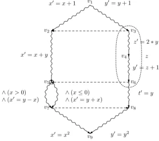
In this paper, we give a formal statement which expresses that a simple and local test performed on every node before its construction permits to avoid the construction of useless

Examples of the results of segmentation of artificial images are shown in Figure 2: (a) an image containing two areas with different statistical characteristics; (b) the result of

The considered scheme of the algorithm for GI (exhaustive search on all bijections that is reduced by equlity checking of some invariant characteristics for the input graphs) may

‫الخــاتمة العامــة ‪:‬‬ ‫يتضق مف خالؿ دراستنا لموضوع االنعكاسات المرتقبة عمى انضماـ الدوؿ النامية في المنظمة‬ ‫العالمية لمتجارة مع اإلشارة إلى

L’archive ouverte pluridisciplinaire HAL, est destinée au dépôt et à la diffusion de documents scientifiques de niveau recherche, publiés ou non, émanant des

L’archive ouverte pluridisciplinaire HAL, est destinée au dépôt et à la diffusion de documents scientifiques de niveau recherche, publiés ou non, émanant des