Detecting Low-Quality Reference Time Series in Stream Recognition

HAL Id: hal-01435197

https://hal.archives-ouvertes.fr/hal-01435197

Submitted on 13 Jan 2017

HAL is a multi-disciplinary open access

archive for the deposit and dissemination of sci-entific research documents, whether they are pub-lished or not. The documents may come from teaching and research institutions in France or abroad, or from public or private research centers.

L’archive ouverte pluridisciplinaire HAL, est destinée au dépôt et à la diffusion de documents scientifiques de niveau recherche, publiés ou non, émanant des établissements d’enseignement et de recherche français ou étrangers, des laboratoires publics ou privés.

Detecting Low-Quality Reference Time Series in Stream

Recognition

Marc Dupont, Pierre-François Marteau, Nehla Ghouaiel

To cite this version:

Marc Dupont, Pierre-François Marteau, Nehla Ghouaiel. Detecting Low-Quality Reference Time Series in Stream Recognition. International Conference on Pattern Recognition (ICPR), IAPR, Dec 2016, Cancun, Mexico. �hal-01435197�

Detecting Low-Quality Reference Time Series in Stream Recognition

Marc Dupont∗†, Pierre-Franc¸ois Marteau∗, Nehla Ghouaiel∗ ∗_{IRISA, Universit´e de Bretagne Sud, Campus de Tohannic, Vannes, France}

†_{Thales Optronique, 2 Avenue Gay Lussac, Elancourt, France}

Abstract—On-line supervised spotting and classification of subsequences can be performed by comparing some dis-tance between the stream and previously learnt time series. However, learning a few incorrect time series can trigger disproportionately many false alarms. In this paper, we propose a fast technique to prune bad instances away and automatically select appropriate distance thresholds. Our main contribution is to turn the ill-defined spotting problem into a collection of single well-defined binary classification problems, by segmenting the stream and by ranking subsets of instances on those segments very quickly. We further demonstrate our technique’s effectiveness on a gesture recog-nition application.

1. Introduction

In the big data context, stream processing has raised recent gain of interest in the research community, although indeed some of the questions it raises have been addressed decades ago. This paper deals with the supervised mon-itoring of data streams in general. However we illustrate our presentation using streams generated by sensors for monitoring users activity or action. We focus essentially on instance based machine learning approaches, where instance means reference pattern that has to be detected and recognized on the fly when it occurs in the stream (”on-line”). More specifically, we address the problem of instance selection with the objective of maximizing the accuracy of the detection and recognition process. Identifying and rejecting ”bad” instances in the training set appear to be of crucial importance. We first give hereinafter a brief highlight of the related work, then detail the main steps of the instance selection algorithm we propose, dedicated to on-line pattern recognition in stream. We finally assess this algorithm on a gesture recognition experiment using a multi sensor data glove.

2. Related work and positioning

A lot of work has been tackled during the last decade in the area of instance selection. In the big data paradigm, instance selection has been addressed through the angle of data reduction to maintain algorithmic scalability, but also to reduce the noise in the training data (1) (2) (3). As the instance selection problem is known to be NP-hard (4), heuristic approaches have been developed, among them evolutionary algorithms have been largely experimented (5). It is quite noticeable that very few of those works, to our knowledge, have specifically addressed the problem

of instance selection in a data stream recognition scheme. Because the processing of streaming data is particularly resource demanding, data reduction and in particular in-stance selection, is a very pressing question. (6) have addressed this issue as an active learning problem in a streaming setting, while mainly considering the detection of mislabeled instances. We also address in this paper the noise reduction angle, although the reduction of the redundancy in the training set is indeed an issue and can be view as an extension of our work. Nevertheless, the noise we tackle is much more located at the feature level rather than at the class variable level.

3. The stream recognition problem

The problem we seek to solve can be formulated as follows. Let(st)be a stream of points that can be infinite in time. For example, this could be a stream of motion values coming from a data glove. Our goal is twofold:

1) spotting: localize meaningful subsequences in this stream, and

2) classifying: label those subsequences with a discrete class label.

In our motion data example, those subsequences could be gestures that we need to both spot and classify, such as, say “hand waving” or “fingers opening”. Throughout this paper, this dual task “spotting + classifying” will be jointly referred to as “recognizing”.

This recognition is done in a supervised manner: be-fore testing, the recognizer is given access to a training stream in which subsequences are all marked with two temporal bounds (for spotting) and a label (for classify-ing), i.e. a tuple(tbeg, tend, `). F It is important to note that

most of the stream points will not be meaningful, in the sense that there is no detection expected. In our gesture example, resting, scratching one’s arm or moving naturally because of walking are three kinds of data that could be considered meaningless because they are not considered explicitly as gestures (assuming they were not explicitly labelled so in the training set). In a way, those meaningless data points can be interpreted as some kind of “silence” (or “noise”).

Another constraint is to design a system that is real time and works on-line, or in a streaming fashion. That is, at testing time, our recognizer must be able to read the incoming data stream and label it continuously; it is not allowed to read the whole stream first and output all subsequences afterwards!

t training stream A B B A _{ground truth} (silence) t testing stream B B A A B B ground truth recognized B A instances extraction

Figure 1. Training and testing a threshold recognizer. All spotted sub-sequences in blue are correct because they each overlap with a ground truth subsequence with the same label.

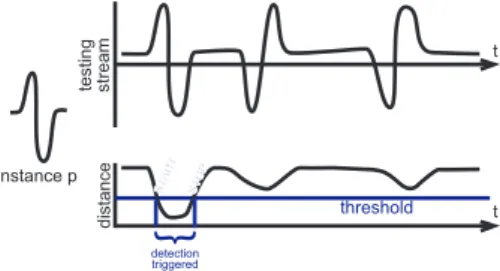
t distance START STOP detection triggered threshold t testing stream instance p

Figure 2. A threshold recognizer triggers detection when distance is under the threshold. While a single instance analysis is shown here, in practice all instances are considered.

The task of the recognizer is, given input points of the un-labelled stream, to emit a START bound when it detects a subsequence (along with the classified label) and a STOP bound when it believes the subsequence is over. Of course, it is difficult to detect a subsequence before it has even started. Hence we do not expect the recognizer to emit the exact ground truth boundaries of the spotted subsequences. We simply say that recognition is correct iff recognized and ground truth subsequences overlap and have the same label, as illustrated in Fig. 1. This is the multiclass recognition problem; unfortunately, notions such as True Negative are not well defined because there is no proper delimitation of the objects to be classified.

4. Threshold recognizer

One simple yet surprisingly effective technique to solve this general recognition problem, that consists in emitting START and STOP bounds, is what we call a threshold-based recognizer. Let’s assume that we have some way of measuring dissimilarity between one learnt time series and the stream at a given point. For example, a well known distance between time series (though not mathematically a distance, it can be intuitively considered as such) exists: Dynamic Time Warping, or DTW (7). It can be easily extended to work in a streaming fashion (8). It has long been known that DTW is very robust for this kind of application, especially when associated to a 1-NN classifier.

Thanks to the continuous distance information describ-ing dissimilarity, we can choose to trigger detection only when an instance gets close enough to the stream. Or, in other words, when one instance’s distance goes under a

t test A A A A t train

Figure 3. Misrecording a single instance can lead to dramatic conse-quences during recognition.

certain threshold. This very simple rule is the essence of what we call the threshold recognizer.

More precisely, the threshold recognizer relies on three internal components. First, a dissimilarity measure (infor-mally referred to as “distance”) between one time series and the stream (for example, a streaming implementation of DTW (8)). Second, a training set of labelled subse-quences (the “instances”). Third, one threshold per class.

A threshold recognizer’s behaviour is as follows:

• for each incoming stream point, compute/update dis-tances between each instance and the stream

• emit START when at least an instance goes under its label’s threshold and emit STOP when no more instance is below threshold

• (advanced: in the case where more than one label is detected, a disambiguation rule such as “pick the label having the closest instance to the stream”) In order to cope with possibly different variances between classes, we pick one threshold per class and not an unique threshold for all classes. To carry on with our gesture detection example, one gesture class could happen to be described by few or no movement (such as “point straightahead”), while another could be very jittery (such as “wave hand”). Time series of the former class will be somewhat static, leading to similar intra-class instances; however, the latter class will have more dissimilar time series because of the high motion.

5. Handling an imperfect training set

Unfortunately, this kind of threshold recognizer has a major drawback. As mentioned above, it takes only one instance to trigger a START bound. What if one instance in the dataset is particularly ”bad”? It might have drastically bad consequences for the whole recognition. Imagine if the user were to record an instance of “wave hand” but accidentally did not wave the hand at the right time: now the dataset would be ”polluted” by an instance labelled “wave hand” whose time series describes the hand resting instead. That would imply that label “wave hand” would be triggered all times where the user rests the hand afterwards! This is an unacceptable price to pay for a single misrecorded instance.

In the following, we describe a procedure to fix this issue, so that a few incorrect instances in the training set

are pruned to avoid harming recognition rates. We wish to jointly discover:

1) subset: which instances should be kept in the dataset (or alternatively: which instances should be removed) 2) thresholds: which thresholds should be given, for

each class.

Those two problems of selecting a subset and setting thresholds might seem to be independent at a first glance, but they are actually highly correlated. Indeed, it might be better to have a low threshold if low-quality instances are going to match too often; or have a high threshold if we know examples will match only when they are expected to. Hence, subsets and thresholds must be analyzed jointly when seeking for optimal recognition rates.

In order to do this, a naive, brute force, strategy would prepare all different subsets and different threshold values, then run the whole recognition procedure for each (subset, thresholds) pair. However, the full recognition procedure: computing all streaming distances, comparing distances and thresholds at each point... is too slow to be run many times. Furthermore, the space or pairs (subsets, thresholds) is enormous; combinations of subsets grow exponentially in the number of instances; and thresholds take continuous values, which already makes exploring their spaces dis-jointly untractable (proved NP-hard (4)), let alone dis-jointly. Rather than analyzing the parameter space naively, we hereby describe a strategy that is much faster and allows for many runs of subset selection in a short period of time. More importantly, it is crucial to observe that our algorithm is not only made for subset + threshold se-lection, but even more: it actually provides the basis for an extremely fast stream analysis in general, able to evaluate the performance of a recognizer on a validation stream and provide in turn accuracy metrics for multiple classes. It does so by turning the ill-defined multiclass stream analysis detection problem, into a collection of binary classification problems, for which notions such as false/true positive/negative measures, etc. are unambigu-ous. This enabled the use of well established metrics and tools that have been known for decades, such as the ROC curve.

6. Overview of the procedure

Before diving into the details of the procedure, we will outline a broad overview of the steps involved.

INPUT:

• Two streams (training and validation) with subse-quence boundaries and labels

OUTPUT:

• high-quality subset of extracted instances

• threshold values

SIDE OUTPUT (optional but possibly useful):

• ranking (ordering) of instances from worst to best • numerical measure indicating how a given subset

per-forms for one class, independently of any threshold selection

STEPS:

1) Extract instances from the training stream.

2) Cut the validation stream into segments, and define expectationsfor each segment.

3) Run the streaming distance on each instance. 4) Find out events between instances and segments, i.e.

when and where they can possibly trigger a recogni-tion. Group events by label and per segment and sort them.

5) Find out the worst candidates; prepare some promis-ing subsets, from which the worst instances are re-moved.

6) Analyze each promising subset on the segments to get a score out of them (very fast). Select the best subset. Select the optimal threshold on this subset.

7. In-depth description

Consider our input data is a labelled stream, that is, a sequence of pointsst∈Rd, wheredis the dimension of the stream, andt = 0, 1, ...T − 1is the time. Usually this stream will represent sampled data acquired by sensors, monitoring metrics, etc. at a regular sample rate.

The subsequences are given as a collection of tuples

(tbeg, tend, `), indicating the beginning and end bound-aries of the subsequence along with its label. We assume subsequences do not overlap.

7.1. Extraction of training instances

For all subsequences (tbeg, tend, `) in the training stream, extract the timeseries betweentbeg andtend, and

store them (see Fig. 1).

7.2. Segmenting the validation stream

The validation stream(vt)is also labelled with a col-lection of tuples(tbeg, tend, `)representing subsequences.

This labelling represents the ground truth where the trained recognizer is expected to spot and classify sub-sequences.

In order to understand why we propose to cut the stream into segments, let’s start by making an essential remark:

An instance will trigger recognition on a segment iff the minimum of its distances on the segment is under the threshold.

It means that instead of analyzing point after point, we can cut the stream into segments, store the minimum for each instance, and then check whether the minimum is under the threshold for the segment! This eliminates an enormous amount of work (Fig. 5).

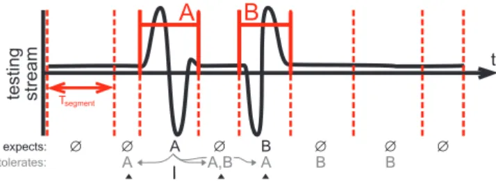
Each segment comes with one “expectation” and a set of tolerated labels (or simply “tolerances”). An expecta-tion is a label `, possibly ∅. If ` 6=∅, then` should be triggered by at least one instance (labelled `) under the threshold. On the other hand, if ` = _{∅, no class should}

be detected, hence all instances should be above their threshold. (Caution: ∅ is just a notation for “no label” and should not be the label of any actual instance.)

Tolerances serve to locally relax recognition con-straints. If a segment tolerates `, then it doesn’t matter

t testing stream Tsegment

A

B

expects: A

A A,B AB B B

tolerates:

Figure 4. Segments delimit labelled subsequences and pieces of unla-belled points (”silence” or ”noise”). Each segment expects a label (or no label) and can optionally tolerate some neighboring labels.

whether`is triggered on this segment: it will never count as a mistake.

With those definitions in mind, let us now describe the segmentation procedure. In order to create the segments, we will simply make cuts. Segments are those portions of time series between cuts:

1) During “silence” (no labelled subsequences), make a cut every Tsegment. Set expectation to ∅ i.e. no label expected.

2) During meaningful subsequences with(tbeg, tend, `),

make cuts attbegandtend(do not sub-cut inside even if longer thanTsegment). Set expectation to label`. Furthermore, for each segment that was created due to a subsequence with label` 6=∅ (rule 2.), we “spread”

`onto neighbouring segments tolerance:

3) If segment sexpects` 6=<sub>∅, add</sub>` to tolerances for segments(s − 1),(s + 1), and(s + 2).

The motivation for spreading tolerances 1 segment on the left and 2 segments on the right is that the streaming distance will usually be sharp to decrease, but will take a bit longer to increase again after recognition and to leave the triggering zone below the threshold. In our experience 1 and 2 have been a good choice, and we believe they should be acceptable for most applications; it is up to the implementer to decide whether to tune those values for their particular task. Also, their effectiveness will depend on the choice ofTsegment.

7.3. Minima computation

Distance computation is the most computing power demanding part of the algorithm. Therefore, we do it as early as possible, only once, and collapse dense distance information into economical representations based on seg-ments and minima.

Let p be an instance of the dataset. The streaming distance is evaluated as discussed in Section 4 (e.g. a streaming implementation of DTW), in order to map each point of the stream vt into a positive real describing the

distance between pand the stream.

However, we do not need to store all distance values. As noted earlier, in order to know if p will trigger on segments, we just need to compare the threshold to the minimumdistance on this segment’s points. Hence, when sliding through the stream vt to compute the distance,

taking note when a segment ends, we only store the

instance p , , , , , , , t distance t stream minima

Figure 5. Minima of distances are sufficient to determine whether an instance will be triggered during an segment.

minimum since it began, and forget other non-minimal values which are useless from now on.

This should yield a sequence mp (“minima”) of

pos-itive numbers where each indexs is a segment and each element mp[s] is the minimum. In terms of memory oc-cupation, it is way more economical to store just minima (as many values as segments) compared to all distances for each timet (as many values as stream points).

All sequencesmp= (mp[s])sshould be computed for each instancep.

7.4. Event computation

As seen in Section 5, threshold adjustment is a matter of compromise between too tolerant (high threshold) and too strict (low threshold) situations. Therefore, in order to set the threshold accordingly, we propose to list events, that is, the segment and threshold at which instances will be triggered (i.e. the minimum of each instance on each segment).

Therefore, an event is a tuple (τ, p, s, g) representing the assertion “On segment s, instance p will trigger its label `(p) at threshold τ, which is g”. The “goodness”

g takes one of two values, GOOD if those labels are the same and BAD otherwise. Also, in the following, we will ensure that if a label ` is tolerated on segment

s, then there are no event linking ` and s, because it is inherently neither good or bad to trigger, or not trigger, a label where it is not expected but tolerated. Note that the trigger threshold for each(p, s)pair is just the minimum of pon s:τ = mp[s].

In order to find out those events, we need to iterate on all instances pand all segmentss:

1) ifs toleratescurrent label`(p), skip this segment. 2) if “labels don’t match”, i.e. (s expects ∅) or (s

expects`s6=∅ and`(p) 6= `s), then register a BAD

event with thresholdmp[s].

3) if “labels match”, i.e. sexpects `s6=∅ and`(p) =

`s, then register a GOOD event with thresholdmp[s]. While looping throughpandsto find out those events, we store them in two data structures:

segment segment mi n ima [1] OK [4] OK [1] no GOOD [4] OK [1] no GOOD [4] 1 BAD [1] OK [4] 1 BAD A ... ... 1 4 expects: mi n ima [1] OK [4] 1 BAD [1] no GOOD [4] 1 BAD [1] no GOOD [4] OK (instance triggers if under threshold) GOOD BAD A ... ... 1 4

Figure 6. EventsE[`, s]for a fixed label` =A and segmentss = 1, 4. We look for an optimal threshold, where there would be at least one GOOD event for segments expecting A, and no BAD event elsewhere. The first situation admits no optimal threshold; however, after removing p2, such a threshold appears.

• Events per label and per segment: let E[`, s] be a vector storing all events whose segment is s and whose instance has label `.

• Bad events per label: letB[`]be a vector storing all BAD events related to instances with label`. An event can be stored duplicated in bothE[`, s]and

B[`].

It is required that each of those individual vectors are sorted by increasingτ value. Intuitively, it provides a way to “slide” from lowest to highest threshold and discover, in order, which kind of event will happen as we increase the threshold. See Fig. 6.

7.5. Promising subsets identification

Identification of promising subsets must be performed independently for all labels. Here, let us focus on a fixed label `, and denote P` the set of all instances with this label.

The vector of bad events B[`], after sorting with respect to increasing threshold, represents a ranking of worst instances of the set P [`]. Indeed, the first ele-ment of B[`]describes which instance will generate the first false positive, as we start from threshold = 0 and increase progressively. This happens precisely because

B[`] is sorted. Therefore, when we want to find which instances are worth removing, looking at B[`] provides us with an ordering of candidates that should be preferred for removal. When a candidate p is removed, it will no more generate a false positive, which in turn allows us to increase the threshold. However, it could turn out to generate a false negative at some other place where this instancepwas needed for the detection. We will take care of this issue in the next section by globally analyzing the performance, on a given class, of removing one or several candidates.

The goal here is to select a good subsetP<sub>`</sub>0⊆ P`. In-stead of brute forcing through all2|P`|_{subsets, we propose}

an efficient strategy (although not theoretically optimal) to prune bad instances. It works in linear O(|P`|) time and thus is tractable even in presence of many instances. The idea is to extract, in order, instances from BAD events inB[`]: say the candidates are, in order,p1, p2, . . .

the subsets we propose are P0

` = {p1, p2, p3, ...}, P`1 =

{p2, p3, ...}, P`2 = {p3, ...}, ..., i.e. P`k is the full set P`

without thekworst instancesp1, ..., pk. These are what we call “promising subsets” and they will be analyzed quickly during the next pass to select the best subset among them.

7.6. Subsets scoring

For a given label `, we consider the binary classifi-cation problem of assigning either label ` _{or ∅ to each}

segment, which expects either`or ∅ (we turn non-`labels into ∅ to focus on` only). Furthermore we consider that we are given a subsetP<sub>`</sub>0of instances. In order to compare those subsets without having to set a manual threshold value, our solution is to compute the ROC (Receiver Operator Characteristic) curve of this binary classification problem and use the AUC (Area Under the Curve) as a quantitative measure to compare subset quality.

In order to compute this ROC curve, the fastest so-lution is to list when each segment will turn from True Negative (TN) to False Positive (FP), or from False Neg-ative (FN) to True Positive (TP). We call those sub-events “switches”. This is easily done: for each segment,E[`, s]

lists the events in order of thresholds; hence the switch event is the event with the lowest threshold (i.e. the first to happen). Thus, it is the first element ofE[`, s] for which the instance p is included in our subset P<sub>`</sub>0. That gives one switch per segment, except for segments tolerating the current label, which do not participate in the binary classification and are simply ignored.

Now that all switches are established, computing the ROC curve and its AUC is as easy as reading the switches in increasing threshold order. A GOOD switch turns FN to TP (up on the ROC curve); a BAD switch turns TN to FP (right on the ROC curve).

Finally, the best subset is the one with the highest AUC. The optimal threshold is selected by finding an optimal point on the ROC curve, but how we define “optimal” does not have a definite answer, so we leave to the implementer the task of choosing their preferred optimal ROC point selection procedure. For example, a simple rule could be selecting a threshold for which the TP rate is higher than some percentage value, say, 95%.

8. Results

We ran our instance selection algorithm on a real-world scenario. It consists of an on-line gesture recog-nition task, captured by a data glove. After some feature engineering, the stream has 13 dimensions related to po-sition, motion, and finger flexion. There are 8 classes of gestures repeated around 4 to 8 times per person. Ges-ture boundaries were added by manual post-processing. Training is composed of 100 Hz streams recorded by two people, totalling 6m40s; testing is composed of 3m04s by a third person.

Some weak instances appear on their own, but in order to better display our algorithm’s value, we further injected “fake” time series in the database, taken by reading a random piece of the training stream and giving it a random

class "faster " 0.2 0.4 0.6 0.8 1.0 0.2 0.4 0.6 0.8 1.0 0 removed ( AUC = 0.43 ) 1 removed ( AUC = 0.7 ) 2 removed ( AUC = 0.9 ) 3 removed ( AUC = 0.96 ) 4 removed ( AUC = 0.99 ) 5 removed ( AUC =1.)

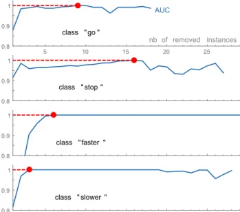
Figure 7. ROC curves for one class of the gesture data set in which fake instances were introduced. The base dataset (”0 removed”) shows poor performance; our method is able to detect the 5 bad instances and enhance the ROC curve as instances are progressively removed from the base dataset. class " go " nb of removed instances AUC 5 10 15 20 25 0.8 0.9 1 class " stop " 0.8 0.9 1 class "faster " 0.8 0.9 1 class " slower " 0.8 0.9 1

Figure 8. Evolution of AUC as low-quality instances are removed. For all classes (including those not shown here due to lack of space), we are able to significantly increase AUC (maximum at red point) compared to the original dataset (leftmost point).

existing label. This makes the task more difficult by lowering the overall dataset quality.

In Fig. 7, we show on a single class that our technique is successful in detecting all bad instances and removing them, attaining here an ideal AUC of 1 (which is an objective that is not always reachable). Plotting the AUC of each ROC curve as we progressively remove instances gives Fig. 8, in which we note that all classes also end up attaining AUC= 1.

Analyzing the dataset on the 3 minute testing stream took only 6.15s on a regular CPU, including extraction, streaming DTW calculation, segmentation, events com-putation and ROC scoring for 215 identified promising subsets.

9. Conclusion

In this work, we have shown that it is advantageous to tackle the multiclass streaming recognition problem as a collection of binary classification problems, one for each class. This interpretation enabled us to derive an original algorithm for proposing jointly efficient (although

sub-optimal) solution to the NP-hard instance selection problem and the threshold tuning. Finally, it allows for the use of ROC analysis in order to detect low-quality instances, and set the distance threshold by selecting the optimal ROC point. The effectiveness of this solution was demonstrated on a real-world recognition task based on glove motion sensors. Finally, running the analysis on segments rather that full stream turns out to be so fast that it opens up the possibility to prune instances in real-time while learning the gestures.

References

[1] J. A. Olvera-L´opez, J. A. Carrasco-Ochoa, J. F. Mart´ınez-Trinidad, and J. Kittler, “A review of in-stance selection methods,” Artif. Intell. Rev., vol. 34, no. 2, pp. 133–143, Aug. 2010.

[2] I. Czarnowski, “Transactions on computational collec-tive intelligence iv,” N. T. Nguyen, Ed. Berlin, Hei-delberg: Springer-Verlag, 2011, ch. Distributed Learn-ing with Data Reduction, pp. 3–121.

[3] Y. Fu, X. Zhu, and B. Li, “A survey on instance selec-tion for active learning,” Knowledge and Informaselec-tion Systems, vol. 35, no. 2, pp. 249–283, 2012.

[4] Y. Hamo and S. Markovitch, “The compset al-gorithm for subset selection,” in Proceedings of The Nineteenth International Joint Conference for Artificial Intelligence, Edinburgh, Scotland, 2005, pp. 728–733.

[5] J. Derrac, S. Garca, and F. Herrera, “A survey on evolutionary instance selection and generation.” Int. J. of Applied Metaheuristic Computing, vol. 1, no. 1, pp. 60–92, 2010.

[6] M.-R. Bouguelia, Y. Bela¨ıd, and A. Bela¨ıd, Pattern Recognition: Applications and Methods: 4th International Conference, ICPRAM 2015, Lisbon, Portugal, January 10-12, 2015, Revised Selected Papers. Cham: Springer International Publishing, 2015, ch. Identifying and Mitigating Labelling Errors in Active Learning, pp. 35–51. [7] H. Sakoe and S. Chiba, “A dynamic programming

approach to continuous speech recognition,” in Proc. of the 7th International Congress of Acoustic, 1971, pp. 65–68.

[8] Y. Sakurai, C. Faloutsos, and M. Yamamuro, “Stream monitoring under the time warping distance,” in Proceedings of the 23rd International Conference on Data Engineering, ICDE 2007, The Marmara Hotel, Istanbul, Turkey, April 15-20, 2007, 2007, pp. 1046– 1055.