Object-Oriented Modeling and Analysis Capabilities

HAL Id: hal-02548276

https://hal.archives-ouvertes.fr/hal-02548276

HAL is a multi-disciplinary open access archive for the deposit and dissemination of sci-entific research documents, whether they are pub-lished or not. The documents may come from teaching and research institutions in France or abroad, or from public or private research centers.

L’archive ouverte pluridisciplinaire HAL, est destinée au dépôt et à la diffusion de documents scientifiques de niveau recherche, publiés ou non, émanant des établissements d’enseignement et de recherche français ou étrangers, des laboratoires publics ou privés.

Object-Oriented Modeling and Analysis Capabilities

Didier Buchs, Mathieu Buffo, Fabrice Kordon

To cite this version:

Didier Buchs, Mathieu Buffo, Fabrice Kordon. Object-Oriented Modeling and Analysis Capabilities. [Research Report] lip6.2000.001, LIP6. 2000. �hal-02548276�

Object-Oriented Modeling

and Analysis Capabilities

CO-OPN to AMInets Task Force

(Didier Buchs1, Matieu Buffo1 and Fabrice Kordon2, in alphabetical order)

1 _{Software Engineering Laboratory, Swiss Federal Institute for Technology,}

1015 Lausanne, Switzerland

{Didier.Buchs,Mathieu.Buffo}@epfl.ch

2_{SRC, LIP6, UMPC - CNRS}

4 Place Jussieu, 75252 Paris Cedex 051015

Fabrice.Kordon@lip6.fr

Abstract. Usual object-oriented modeling notations have either high expressiv-ity, or a high proof-potential. As a consequence, developers have to choose between an easy modeling or good analysis capability. This paper proposes to bridge the object-oriented modeling language CO-OPN with the Petri-net based formalism AMI-nets. Hence, user can manipulate easy-to-use, expressive CO-OPN models, while keeping high proof-potential thanks to AMI nets.

1 Introduction

Development and maintenance of industrial applications becomes more and more difficult. Systems’ complexity increases [19], technologies evolve, requirements has to take care of «social factors» [12] and products’ time to market reduces. Instead of «software crisis», people are now speaking of «software chronic crisis» [11]. Estima-tion costs of such a crisis have been estimated to $ 100 billion in 1996 [27].

One problem in implementing systems is its evaluation. Post implementation test-ing is not reliable because it is impossible to cover all possible executions of complex systems. Software modeling through Object Oriented approaches such as OMT or UML appears to be a solution to this problem. However, these description languages essentially focus on the description of a general solution. Then, the system still has to be analyzed.

Analysis could be supported by formal methods that are known to bring safe eval-uation techniques, due to their mathematical foundation [20, 21]. However, these mathematical foundations also bring problems like:

• Formal notation is alien to most practicing programmers, who have little training in higher mathematics,

• Even if mathematical notations are very general, they require discrete types of methods for discrete application domains. Thus, the same notation can be used in many ways; this implies discrete evaluation and proof methods,

• It is difficult to integrate formal methods into industrial software processes because the notation used contain many mechanisms that are difficult to use, • Many of the most popular formal methods do not scale up to practical-size

prob-lems.

Thus, it appears that formal methods cannot be directly used to validate large indus-trial-like systems. They have to be manipulated via high level representations.

This paper proposes to bridge the object-oriented Petri nets based specification language CO-OPN with the Petri net model of the CPN-AMI environment (AMI-Nets) to provide an approach dedicated to the analysis of concurrent systems. Hence, users can manipulate high-level representations in CO-OPN, while discrete evaluations and proof methods are likely to be performed on AMI-Nets using CPN-AMI. Section 2 introduces the various models and notations used in this work. Section 3 presents the current stage of the bridge between CO-OPN and AMI-Nets. Then, sections 4 and 5 illustrate our approach by means of two discrete examples focusing on two different aspects of concurrent systems. Finally, section 6 concludes the paper.

2 Software Modeling

It was mentioned in the introduction that one problem in implementing software reside in their evaluation. One way - promoted by Software Engineering - to meet this challenge is to develop software models before the definitive product. These software models can be used to validate user requirements, to derive early prototypes, and finally to evaluate the various possible solutions. Actually, analyzing software models is one of the key task of software development process.

Software models usually include descriptions of the main features of the proposed software, defined in a suitable modeling language or notation. Actually, we feel that good modeling languages have an ability to abstract - at least intuitively, for the devel-opers - marginal but rather complex implementation details.

Among the various modeling notations used yet, we propose to have a look at three typical notations, namely UML, Petri nets and algebraic abstract data types. • UML [25] (Unified Modeling Language), proposed by OMG (Object

Manage-ment Group), is becoming the current leader among the modeling languages for object-oriented systems. UML models are composed of various graphs, defining classes, objects and messages composing the models.

• Petri nets are a convenient way to describe software models based on the intuitive notion of state machines. In short, a Petri net is a notation relying on places, con-taining the resources of the system, and transitions, reflecting the interactions among the resources. With regards to automata, Petri nets are much more easy to use, much more intuitive, because the coordination between the various parts of the system are explicitly represented.

• Algebraic abstract data types are a formal modeling notation based on a sound mathematical background. In short, such models, called algebras, are induced by a set of axioms, formalizing the desired properties.

2.1 Expressiveness Power versus Analysis Capabilities

Let us consider discrete approaches and notations family. We could class them using three criteria:

• structuration potential: this criterion requires the associated notation to provide high level structuration capabilities, like an object model (classes, inheritance etc.), a module approach, and so on;

• verification potential: this criterion requires strong foundation to provide execu-tion of a specificaexecu-tion, model checking and even structural analysis of a system model;

• ease to verify: this criterion requires that the verification potential is likely to be performed using simple techniques and tools

Fig. 1. shows how some usual notations can be classified according these three criteria. OMT or UML provide good design capabilities but are very poor in terms of verification that is mostly cross review by humans or simulation (usually ease to pro-duce). On the other end, notations such as Petri nets or algebraic specifications have strong formal verification capabilities with average ease-to-verify; however these nota-tions lack high-level structuring capabilities and it is difficult to handle complex speci-fication such as the one of industrial applications. Some extensions to formal methods are often investigated like CO-OPN and other Object-Oriented Petri Nets [14, 18, 2]. The main problem of such formalisms is to catch up with formal properties: small modifications induce theoretical problems that are still to be solved. Thus, even if these formalisms have a good structuration potential and a good verification potential, they have a rather low ease to verify evaluation.

Fig. 1. A classification of specification notations.

UML, OMT, etc.

CO-OPN Petri Nets, Alg. Spec. Structuration potential Verification potential Ease to verify

2.2 Association of UML, CO-OPN and AMI-Nets

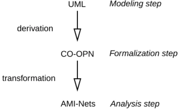
Our approach is based on several refinement steps. Each one is dedicated to a main goal and relies on an appropriate formalism. Fig. 2. illustrates our process. First, modeling is performed using a suitable modeling language like UML [25]. This is done according to a given method like FUSION [8]. Then, the second step resides in the derivation into a high level formal notation for object oriented modeling: CO-OPN. Finally, the last steps consist in transforming CO-OPN into AMI-Net: a formal specifi-cation suitable for supporting the proof process. AMI-Net is a Petri net dialect having the expression power of Well-formed nets [6].

Fig. 2. provides a more synthetic view the proposed procedure. Our aim is to safely derive distributed programs from UML models. Both formalization and analy-ses steps allows the exploitation of formal methods. This enables the validation of the UML model and verification its formalization (using Petri nets). It also allows us to take into consideration formal properties to optimize the resulting program.

Fig. 2. also shows the path from a specification level to another one. One CO-OPN specification is derived from an UML specification. On the contrary, several Petri Net specifications are derived from CO-OPN. Each one represents one particular aspect of the CO-OPN model and is dedicated to the verification of a given property. Implementation of CO-OPN modules into programs takes benefits from this analysis.

The first step now is to briefly describe the basics of CO-OPN and AMI-Nets as well as the features of CPN-AMI. Then we have to present the translation strategy between both formalisms we use. Finally - and archetypally - we illustrate our approach by means of two paradigmatic case studies. These case studies are very sim-ple but cover a substantial part of the main concepts of CO-OPN.

The goal of the first case study is the modeling of a simple communication proto-col. It allows the analysis of the various components involved in the system, the analy-sis of their instantiation, their composition, their synchronization. The second case study deals with the modeling of an accumulator component. It focus on the

deploy-Fig. 2. Chaining formalisms over the proposed approach.

AMI-Nets UML CO-OPN Modeling step Formalization step Analysis step derivation transformation

ment of complex object synchronizations (in particular, sequential recursive method calls) and the management of algebraic data types.

2.3 CO-OPN

CO-OPN is an object-oriented modeling language, based on Algebraic Data Types (ADT), Petri nets, and IWIM coordination models [5]. Hence, CO-OPN con-crete specifications are collections of ADT, class and coordination modules [3, 4]. Syn-tactically, each module has the same overall structure; it includes an interface section defining all elements accessible from the outside, and a body section including the local aspects private to the module. Moreover, class and context modules have conven-ient graphical representations, showing their underlying Petri net model. Low-level mechanisms and other features dealing specifically with object-orientation, such as genericity, sub-classing and sub-typing are out of the scope of this paper, can be found in [3].

ADT Modules. CO-OPN ADT modules define data types by means of algebraic

specifications. Each module describes one or more sorts (i.e. names of data types), along with generators and operations on these sorts. The exact definition of the opera-tions is given in the body of the module, by means of equationnal axioms. For instance, Figure 3 describes a (very simple) ADT defining one sort (the booleans) and one oper-ation on this sort (the negoper-ation).

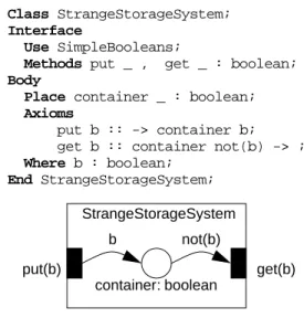
Class Modules. CO-OPN classes are described by means of modular algebraic Petri

nets with particular, parameterised, external transitions, the methods of the class. The behaviour of transitions are defined by so-called behavioural axioms, corresponding to the axioms in ADT. A method call is achieved by synchronizing external transitions, according to the fusion of transitions technique.

Below is the code and the associated Petri net graphics of a class modeling an unusual storage system; it stores boolean values, but delivers the negated ones. The interface defines two methods, for the storage and the retrieving of values. The body is actually a textual representation of the associated Petri net. Free variables may be defined and used in the behavioural axioms.

ADT SimpleBooleans; Interface

Sort booleans;

Generators true, false : ->boolean; Operation not_ : boolean->boolean; Body

Axioms

not (true) = false; not (false) = true; End SimpleBooleans;

Coordination Modules. A third kind of modules is present in CO-OPN, the context modules [5], which share the same overall structure with ADT and class modules. Basically, context modules allow the modeling of distributed systems, by means of suitable coordination mechanisms, more complex than the fusion of transitions seen above. As context modules are clearly specific to the coordination theory, they are not illustrated here.

2.4 AMI-Nets

AMI-Nets are a Petri Net dialect having an expression strength equivalent to the one of Well-formed nets [6]. They include, besides the graphical features of a Place/ Transition Petri net (places, transitions and arcs) textual information like:

• place and transition domains, and transition guards, • an enriched syntax for arc labels and place markings,

The behavior of an AMI net is controlled by the same set of rules used for general colored nets:

• A domain is associated with each place and transition of the model. Elements of these domains are called colors.

• When firing, a transition is binded by an element of its domain.

• Each token in a place is colored by an element of the place domain (several tokens may have the same color). The marking of a place is thus a multiset of colors - a set in which an element may occur several times.

• For a binded transition to be enabled, each input place of the transition must con-tain a sufficient (possibly null) number of tokens for every color of the place domain. These tokens will be taken from the place when the transition fires. Sim-ilarly, the firing will produce colored tokens in the output places of the transition.

Class StrangeStorageSystem; Interface

Use SimpleBooleans;

Methods put _ , get _ : boolean; Body

Place container _ : boolean; Axioms

put b :: -> container b; get b :: container not(b) -> ; Where b : boolean;

End StrangeStorageSystem;

Fig. 4. Class StrangeStorageSystem

StrangeStorageSystem

container: boolean

put(b) get(b)

Like in Ordinary Petri nets, the label attached to the arcs determines the number of tokens to be taken or produced. However, this label is now a color function that associates a multiset of colors of the place domain with each binding of the transi-tion.

• Independently from the evaluation of the color functions, a transition may not be enabled if its binding does not satisfy some predicate. This predicate is called the guard of the transition.

2.5 The CPN-AMI environment

CPN-AMI [22] is a collection of tools federated in FrameKit [16], a generic CASE environment offering both integration capabilities and an enhanced develop-ment environdevelop-ment. As all CASE environdevelop-ments generated from FrameKit, CP-AMI offers a user-friendly access to Petri net services through a unique user interface: Macao [23].

This architecture is one of the strongest points in CPN-AMI. It enables an enrich-ment process taking benefits of other developenrich-ments to propose a unified Petri net based environment. Enrichment of the successive versions of CPN-AMI was done at a rela-tively low development cost.

The current version of CPN-AMI offers numerous services such as: • Modeling tools:

- Syntactic verifier: checks the AMI-Net syntax and transform the Petri net into an internal representation.

- Modular Petri net assembling: this tool is built to help designer to assemble modules communicating either by means of places or by means of transitions. The users select a group of objets and then, merge them to one equivalent object if it is possible (for example, color domains are the same for places).

- Pretty Petri Nets: this service aims to rearrange "spaghetti" Petri nets. This serv-ice has been made to be exploited by other Petri net servserv-ices (like CPN-Unfolder, Prefix or reachability graph display). However, it can be directly invoked by a user. This service relies on DOT [17].

- Suppression of 0-bounded places and non-firable transitions: uses the bound of place service to suppress 0-bounded places and transitions with those places as precondition. Mainly used with structural analysis in order to limit the study to the useful part of the net.

• Simulation and debugging:

- Colored Petri net simulator: in this tool, we have attempted to keep, as more as possible, the analogy with programming language debuggers. To achieve this goal, the user may use different execution modes, break point possibilities, data extractions during the execution and external treatments associated to transition. Standard debugging functions are also available like intermediate state manage-ment (including load and save operations) and configuration managemanage-ment (a configuration is a set of simulation parameters: scripts definitions, observation

net, intermediate state). • Structural analysis:

- Boolean formula on reachability graph: this tool computes a set of markings containing the reachability set. In this set, places are just considered as “marked” or “unmarked”. The results are displayed as properties over the net. This service uses BDDs [24] to compute the marking set.

- Bounds of places: this tool computes lower and upper bounds. The calculus is based on the state equation and uses linear programming techniques. As a con-sequence, the computed bounds (higher and lower) may not be the best ones, but this tool may be useful to quickly highlight some major problems in the model. For colored models, this tool can be accessed via P/T unfolding. This service is based on lp_solve (ftp://ftp.es.ele.tue.nl/pub/lp_solve).

- Place invariants: computation of P-SemiFlows using a service from GreatSPN [7].

- Colored place invariants: this tool computes invariants using a adaptaed version of the general algorithm [9]. It is one of the very few implemented ones. - Transition invariants: computation of T-SemiFlows using a service from

Great-SPN.

- Siphon and deadlocks: they can be computed using a service from GreatSPN or using a BDD based implementation.

- Liveness computation: computes if the net is live (from any reachable state and for any transition it is possible to reach a state from which the transition is fira-ble).

- Linear properties characterization: the aim of this tool is to compute a linear characterization of the reachability set. When the resulting linear constraints system exactly describes the reachability set, a message warns the user.

- Colored Petri net unfolding: transforms a colored Petri net into a Place/Transi-tion Petri net. The resulting net is a new model that can be displayed and ana-lyzed. An option allows to suppress 0-bounded places and non-firable transitions. This option uses a heuristic to compute those places (it is not based, like the “suppression of 0-bounded places and non-firable transitions” service, on linear programming). Another option allows to compute a pretty layout of the resulting net.

- McMillan unfolding: this service computes an unfolding for a safe net (safety is not verified by the tool). This software has been developed by S. Römer (from Technische Universität München) and implements the algorithm defined by J. Esparza, S. Römer & W. Vogler in [10]. This tool is also part of PEP [13]. • Model checking:

- Generation of the reachability graph, CTL and LTL queries evaluation: this tool is based on PROD [28].

- Generation of the symbolic reachability graph: This service is based on a serv-ice in GreatSPN. A Symbolic Reachability Graph (SRG) is a highly condensed representation of the reachability graph built automatically from a specification of system in terms of Well-formed net. The building of such graph profits from the presence of object symmetries to aggregate either states or actions within

symbolic representatives (equivalence classes). The equivalence relation between states is based on structural symmetries that are directly read off from the types of objects defined in the system specification. By defining convenient types of actions for these types of objects, it can be ensured that states that are equivalent let the future behavior of the system unchanged

3 Translation Strategies and Rules

One of the key aspect of our work is to be able to translate a CO-OPN specifica-tion into a model more suitable for the analysis of properties. Hence, it is a way to extract properties of CO-OPN specification without paying the price of analyzing the original CO-OPN model. Then, properties computed on the «analysis model» can be interpreted in the CO-OPN model. Petri nets are suitable as the analysis model. To sup-port the analysis of specification, we have chosen AMI-Net. Thus, the Petri net dialect we have selected is AMI-Net.

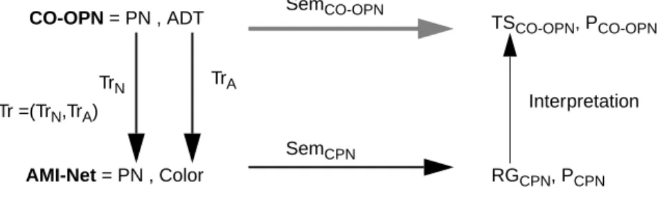
Fig. 5. shows a typical translation scheme. The translation process has to cope with the two aspects of CO-OPN (Petri nets and Algebraic data types, respectively noted PN and ADT on the Figure). Please note that, due to the expressiveness of CO-OPN, we consider several translation schemes. Each one is dedicated to the verifica-tion of particular properties.

The gray arrow in Fig. 5. corresponds to the difficult way of proving a CO-OPN specification. Hence, we exploit the correspondence between CO-OPN and AMI-Nets. For some properties we aim to prove, we can find a translation such that the interpretation of AMI-Net properties is included in (i.e.

), where is such that

.

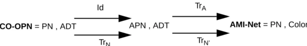
Therefore, our goal is to find suitable transformations between CO-OPN and AMI-Nets. We decompose this transformation in two discrete steps. The first one is devoted to the translation of CO-OPN systems into standard (i.e. un-synchronized) algebraic Petri nets (APN)[29, 26], while the second one is dedicated to the translation

Fig. 5. The translation scheme.

CO-OPN = PN , ADT _TS CO-OPN, PCO-OPN AMI-Net = PN , Color RG_CPN, P_CPN Tr_N TrA Sem_CO-OPN Sem_CPN Interpretation Tr =(Tr_N,Tr_A) P_valid⊆P_CO–OPN Tr P_valid Interpretation P( _CPN)⊆P_valid P_CPN Sem_CPN(Tr CO( –OPN)) = (RG_CPN,P_CPN) Tr

of algebras into colors. This situation is suggested in Fig. 6.

The following sections present the key problems of the transformation process from CO-OPN to AMI-Nets, as well as its limitations. We now provide translation rules for the synchronization operations, as well as those dealing with axioms (recur-sive definitions, classes and algebraic values, etc.).

The detail of the translation between CO-OPN and algebraic net is given in Fig. 7. The translation is divided into two parts, the first is the construction of the computation of the transaction by sub-nets. Each sub-net being connected to each other by fusion of transition, the second step is the interpretation of the fusion operators in order to pro-duce the resulting algebraic net..

First of all, we must provide a simplified but formal description of the CO-OPN notations, needed for the description of the translation rules. Given an algebraic speci-fication , given a set of places , a set of transitions and a set of behavioural

axioms denoted by where is a

transi-tion, is a synchronization built over transitions by the simultaneous, sequential and alternative operators:

(1) (2) (3) (4) If and are markings over the set of places , a CO-OPN specification is:

(5) Given axioms of form , we define an algebraic net as:

Fig. 6. Detail of the CO-OPN to AMI-Nets translation.

Fig. 7. Detail of the CO-OPN to Algebraic net translation TrN.

CO-OPN = PN , ADT APN , ADT Tr_N

Id

AMI-Net = PN , Color

Tr_N’ Tr_A

Axiom_CO-OPN <Axiom_APN,FusionOpSet>

Tr TrBox

Axiom_APN

Inter

ADT P T

Axioms_COOPN t with sync : pre→post t∈T sync∈Sync t∈T⇒sync∈Sync s s', ∈Sync⇒s // s'∈Sync s s', ∈Sync⇒s + s'∈Sync s s', ∈Sync⇒s ... s'∈Sync pre post P

Spec_COOPN = 〈P T Axioms, , _COOPN, ADT〉

(6) Before going deeper into details about transformations , and , we briefly introduces now the concepts of transactions how they are seen in COOPN -and transition fusion.

3.1 Synchronizations as Transactions

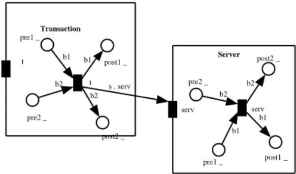
CO-OPN synchronizations can be considered as nested transactions. Therefore, we first describe how a single synchronization can be translated into a transaction using standard Petri net features. Fig. 8. shows an example of synchronization, where transitions and are fired simultaneously, as a transaction.

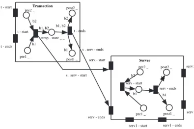
Fig. 9. shows the result of our translation procedure. we split transition t into two transitions: and , representing respectively the beginning and the end of the transaction. Both transitions are fired sequentially. A similar transformation is applied to transition serv. To respect the transaction concept, is associated with and is associated with . Both associations are accomplished by applying the transition fusion principle [1].

Fig. 8. Example of CO-OPN synchronization.

Spec_APN = 〈P T Axioms, , _APN, ADT〉

TrBox Tr Inter t serv Transaction t pre1 _ post1 _ pre2 _ post2 _ t b1 b2 b1 b2 s . serv Server serv pre1 _ post1 _ pre2 _ post2 _ serv b1 b2 b1 b2 Tstart Tend Tstart

3.2 Transition Fusion

In order to collect the set of all the necessary fusion of transitions in , we define the syntactic fusion operator, denoted by , with the following profile:

(7) The semantic of the fusion of transition consists in the union of all the sets represent-ing pre- and post-conditions of transitions involved in the fusion operation. This obviously produce a new pre- and post-condition, associated to the new transition denoted by .

We are now able to express the transition fusion that is needed when decomposing CO-OPN synchronizations using our syntactic operator. The interpretation of this syn-tactic operator on a set of axiom is given by the operation, defined as follows:

(8) (9)

where and .

This operator is the basis of the translation of CO-OPN into algebraic nets. Never-theless all problems are not solved yet, as the following remaining questions should be stated:

• How to manage algebraic terms? (variables must convey the values)

• How to deal with the multiplicity of the axioms? (it is mainly a combinatorial expansion of the fusion)

These questions will be illustrated through paradigmatic examples.

Fig. 9. Translated synchronization.

Transaction t - start t - ends pre1 _ post1 _ pre2 _ post2 _ temp - state _ _ t - start b1 b2 b1, b2 s . serv - start t - ends b1, b2 b1 b2 s . serv - ends Server serv - start serv - ends

serv1 - start serv1 - ends serv2 serv2 pre1 _ post1 _ pre2 _ post2 _ serv - start b1 b2 serv - ends b1 b2 T FusionOpSet

name # name₁...name_n∈Tn+1

name_i name

Fusion

Fusion : ℘(Axiom_APN)×FusionOpSet→℘(Axiom_APN) Fusion Ax name # name( , ₁...name_n) = Ax∪{name : pre→post} pre Pre Ax namei( , )

0< <i

∪

= post Post Ax namei( , )

0< <i

∪

3.3 Translation of Synchronization Expressions:

We define the translation operation acting on synchronization expressions: (10) This operation is defined with the rule dealing with simple coercion, and recursively by the rules , and dealing with simultaneity, sequentiallity and non-determinism respectively. The translation produces axioms, operators of fusion, and transitions. Actually, the translated elements can be seen as a kind of box, with two transitions generically called and (The last two elements in the operation profile) acting as connectors. The semantics of these boxes must be inter-preted as follows: the synchronization is fire-able if there exist - in the semantics of the translated net - a fire-able sequence of transitions, the first element of which is and the last element .

The rule for a simple coercion , called is defined as follow (we assume that transitions and are new for each application of the rule):

(11)

The rule for the simultaneity of synchronizations and , called , is defined as follow (we assume that each application of the rules produces new items ,

, , and ):

(12) Where:

and

The rule for the sequentiality of synchronizations and , called , is defined as follow (we assume that is the generic name for un-named transitions, and that each application of the rules produces new items , , , ,

, , , and ):

(13) Where:

TrBox

TrBox : Sync→Axiom_APN×℘(FusionOpSet)×T×T

Trans Sim Seq Alt

Tstart Tend

Tstart Tend

t Trans

Tstart Tend

TrBox t( )=〈∅ ∅, , Tstart Tend, 〉

--- Trans

s s' Sim

Tstart Tend temp Sseq₁ Sseq₂

TrBox s( )=〈Ax Fus Sstart Send, , , 〉,TrBox s'( )=〈Ax' Fus' S'start S'end, , , 〉 TrBox s // s'( )=〈newAx newFus Tstart Tend, , , 〉

--- Sim

newAx = Ax∪Ax'∪{Sseq₁ : →temp}∪{Sseq₂ : temp→ }

newFus = Fus∪Fus'∪{Tstart # Sstart S'start Sseq₁}∪{Tend # Send S'end Sseq₂}

s s' Seq

ε

Tstart Tend tem p₁ temp2 tem p₃ Sseq₁ Sseq₂ S'seq₁ S'seq₂

TrBox s( )= 〈Ax Fus Sstart Send, , , 〉,TrBox s'( )=〈Ax' Fus' S'start S'end, , , 〉 TrBox s ... s'( )= 〈newAx newFus Tstart Tend, , , 〉

--- Seq

newAx = Ax∪Ax'∪{Sseq₁ : →tem p₁}∪{Sseq₂ : tem p₁→tem p₂}

and

The rule for the non-deterministic choice of synchronizations and , called , is defined as follow (we assume that is the generic name for un-named transi-tions, and that each application of the rules produces new items and ):

(14) Where:

It must be noted that recursive definitions are not covered by . Hence, we propose to handle recursivity through net expansion; each level of recursion implies the adding of new transitions in the translated net. For instance, consider the example depicted in Fig. 10. showing iterators on naturals. The simple net is translated and expanded for two levels of recursion. newFus = Fus∪Fus'∪{Tstart # Sstart Sseq₁}∪{ε # Sseq₂ Send}

∪{ε # S'start S'seq₁}∪{Tend # S'end S'seq₂}

s s'

Alt ε

Tstart Tend TrBox s( )= 〈Ax Fus Sstart Send, , , 〉,TrBox s'( )=〈Ax' Fus' S'start S'end, , , 〉

TrBox s + s'( )=〈Ax∪Ax',newFus Tstart Tend, , 〉

--- Seq

newFus = Fus∪Fus'∪{Tstart # Sstart}∪{Tstart # S'start}

∪{Tend # Send}∪{Tend # S'end} TrBox

3.4 Translation of Synchronizations:

CO-OPN introduces synchronization between transitions by means of the abstrac-tion operator called . This operator links an event (in other words, a local transi-tion) and a synchronization expression, the translation of which is given above.

We define the translation operation acting on axioms, including the synchroni-zations:

(15) This operation is defined with the rule dealing with axioms including

syn-t: Naturals;

t(succ(n)) with t(n): pren -> postn; t(0) : pre0 -> post0;

Produces, for two iterations:

t(succ(n)): n= succ(m) & m = 0 =>

pren/1,pren/2,pre0 -> postn/1,postn/2,post0; t(succ(n)): n= 0 => pren/1,pre0 -> postn/1,post0; t(0) : pre0 -> post0;

Which can be reduced by replacing equal by equal:

t(succ(succ(0))):

pren/1,pren/2,pre0 -> postn/1,postn/2,post0; t(succ(0)): pren/1,pre0 -> postn/1,post0;

t(0) : pre0 -> post0;

Produces for 2 iterations and transition splitting:

t-start(succ(n)) : n= succ(m) & m = 0 =>

pren/1,pren/2,pre0 -> temp1 n, temp2 m, temp0; t-ends(succ(n)):

temp1 n ,temp2 m, temp0-> postn/1,postn/2,post0; t-start(succ(n)) : n = 0 =>

pren/1, pre0 -> temp1 n, temp0;

t-ends(succ(n)): temp1 n, temp0 -> postn/1, post0; t-start(0) : pre0 -> temp0;

t-ends(0) : temp0 -> post0;

Which can be reduced by replacing equal by equal:

t-start(succ(succ(0))) : pren/1,pren/2,pre0 ->

temp1 succ(0), temp2 0, temp0;

t-ends(succ(succ(0))): temp1 succ(0) ,temp2 0, temp0 -> postn/1,postn/2,post0;

t-start(succ(0)) : pren/1, pre0 -> temp1 0, temp0; t-ends(succ(0)): temp1 0, temp0 -> postn/1, post0; t-start(0) : pre0 -> temp0;

t-ends(0) : temp0 -> post0;

Fig. 10. Iterator on Naturals

Tr

With

Tr

Tr : Axiom_COOPN→Axiom_APN×℘(FusionOpSet)

chronization, and with the rule , taking care of un-synchronized axioms. The rule is defined by the following rule (we assume that each application of the rules produces new items ):

(16) Where:

and

The rule is defined by the following rule (we assume that each application of the rules produces new items ):

(17) Where:

and

3.5 Interpretation of the fusion:

The translation function does not ensure the computation of all axioms. It is necessary to perform an interpretation of the transition fusion, as collected in the sec-ond component of the result of . This is done by the interpretation operation which is based on the interpretation of the operator seen above, acting on axi-oms. Formally, we define the interpretation operation:

(18)

3.6 Recursive Definitions

The interpretation operation , as seen above, do not cover recursive defini-tions. We propose, for now, to manage recursivity by admitting a bound to the execu-tion of the recursive synchronizaexecu-tions, and by adopting ad-hoc techniques to avoid conflicts between the partially computed data resulting from the various level of

recur-WithNoSync With

temp

Tr Ax( )=〈Ax₁,Fus₁〉,TrBox s( )=〈Ax₂,Fus₂, Sstart Send, 〉 Tr Ax( ∪{t withs : cond⇒pre→post})=〈newAx newFus, 〉

--- With

newAx = Ax₁∪Ax₂∪{Tpre : cond⇒pre→temp}∪{Tpre : temp→post}

newFus = Fus₁∪Fus₂∪{Tstart # Tpre Sstart}∪{Tend # Tpost Send}

WithNoSync

temp Tr Ax( )=〈Ax₁,Fus₁〉

Tr Ax( ∪{t : cond⇒pre→post})= 〈newAx newFus, 〉

--- WithNoSync

newAx = Ax₁∪{Tpre : cond⇒pre→temp}∪{Tpre : temp→post}

newFus = Fus₁∪{Tstart # Tpre Sstart}∪{Tend # Tpost Send}

Inter

Tr Inter

Fusion

Inter : Axiom_APN×℘(FusionOpSet)→Axiom_APN

Inter(〈Ax Fus, 〉) Inter(〈Ax∪{ }f ,Fus–{ }f 〉) if f∃ ∈Fus, f ={t # t1 ... tn}

Ax else      = Inter

sion.

Hence, we should obtain an approximation of the original semantics, with a static limit in the re-application of recursive synchronizations. For a set of axioms , we denote by the new set of axioms reflecting this process of recursion reduc-tion. Many work must still be done in this area of investigations; we just can cite now the following conjecture:

Conjecture of Buchs: 3.7 Templates

Class information are modelled by cartesian products of object references and values. Methods include an additional parameter representing the object on which the method is applied.

3.8 Taking into account Algebraic value in the Translation

The rule presented before must include algebraic value management, this is nec-essary for keeping the same value for the variable in the t-start and t-end variables. Intermediate place must be a cartesian product of the values of all the variables used in both t-start and t-end axioms.

3.9 Unfolding of Behavioural Axioms

In the axioms it is possible to unfold the conditions and parameter passing accord-ing to the algebraic definitions. This process splits behavioural axioms in various cases corresponding to the case of the algebraic definitions of the operators. This unfolding is generally infinite; bounds must be fixed depending on the interest of this decomposi-tion. Unfolding can also be applied on selected operators depending on the goal of this unfolding.

4 Case study 1: Communication Protocol

The first case study deals with a communication protocol problem and illustrates the efficiency of both CO-OPN and Petri nets to extract accurate information suitable for a final implementation.

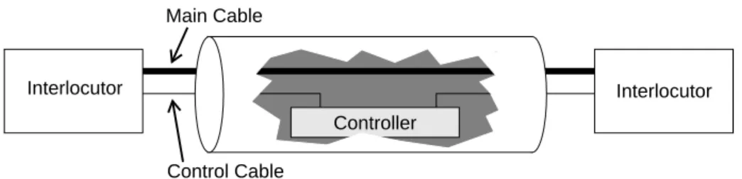
We would like to design a safe channel based on a single cable line. The usual problem with a unique cable is that electric signals coming from various origins may provoke collisions (message is lost). To ensure a safe communication on the channel, we propose the architecture of Fig. 11.

The channel relates two interlocutors that communicate together. It is composed of a control cable and a controller that manages shared access to the channel main

Ax Ax_PART

cable (128 bits width). The controller is connected two each interlocutor with a dis-crete control cable (3 bits width). There is one control cable per interlocutor. Interlocu-tors cannot send a signal at the same time : they must ask first the line to the controller that accepts or refuse (according to an implemented strategy).

Interlocutors have to respect the following protocol:

(1) the default state for an interlocutor is listening to the main cable, (2) when it wants to emit a signal, the interlocutor asks for the main cable,

(3) if the controller provides the main line, then, the interlocutor sends its message and waits for an acknowledge,

(4) if the controller refuses the main line, then the interlocutor cannot get the line and should retry and retries later on,

(5) interlocutors only send one message at a time,

(6) when an interlocutor gets its acknowledge, it frees the line for another use, (7) Only messages passing through the main cable are acknowledged, (8) The control cable is secure,

(9) Signal on the main cable can be lost; however, we assume that connection between the two interlocutors cannot be cut (message loss is bounded).

The table above provides the identification of signals passing through the cables.

A typical execution scenarios is provided hereafter to illustrate the expected behavior of a interlocutor according to specific situations.

Fig. 11. Structure of the line that composes a safe channel.

Signal name

Signification Signal direction

Interlocutor Controller

AMC Ask for main cable ®

RMC Refuse main cable √

PMC Provide main cable √

MSG Message √ ®

ACK Acknowledge √ ®

FMC Free the main cable ®

Fig. 12.

Interlocutor _Interlocutor

Controller Main Cable

Fig. 13. illustrates the behavior of a interlocutor that initiates a communication when the controller provides the main cable. Then, the answer to AMC (demand) is PMC. The interlocutor (here, 1) then sends the message to the other interlocutor (here, 2) and waits for an acknowledge. When it gets the acknowledge, it releases the main cable (FMC).

Let us state some properties we would like to verify on this system: (i) the controller can never provide the line to more than one interlocutor,

(ii) when an interlocutor decides to send a message, the other one always get it soon or later.

4.1 The CO-OPN model

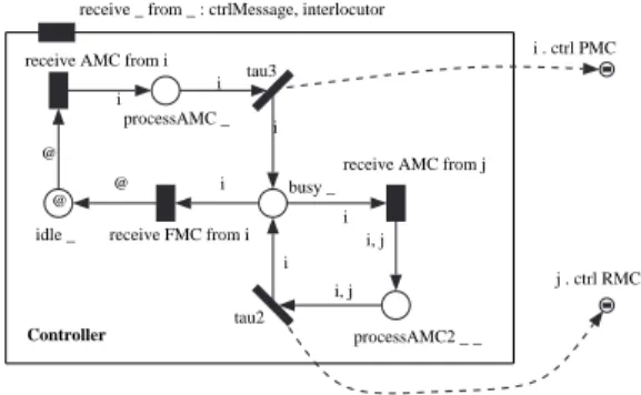
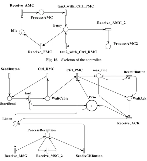
The CO-OPN model is composed of two classes, representing the controller and the interlocutors. The controller class is rather simple, as shown in Fig. 14. It includes two places denoting an idle and a busy state. Receptions of AMC and FMC trigger the switch from a state to another. In addition, a reception of AMC in busy state triggers the emission of a RMC.

The case of the interlocutors is more complex, as shown in Fig. 15. In essence, an interlocutor is composed of two parallel processes; the first process cares about the reception of messages, while the second one cares about the emission.

The reception process, shown on the bottom of the figure, is a simple sequence of mes-sage’s reception, repetions of mesmes-sage’s receptions (due to signal lost, an

re-emis-Fig. 13. UML-like sequence diagram of an accepted connection

Fig. 14. CO-OPN description of the controller.

interlocutor_2 controller FMC interlocutor_1 ACK MSG PMC AMC Controller

receive _ from _ : ctrlMessage, interlocutor

idle _ @

processAMC _ busy _

processAMC2 _ _ receive AMC from i

@ i tau3 i i i . ctrl PMC

receive AMC from j i i, j tau2 i, j i j . ctrl RMC receive FMC from i i @

sions), and finally an ACK emission.

The emission process starts by asking the controller for the main cable, followed either by RMC an retries, or by PMC and the message’s emission. At this time, the reception process is stopped (the token in place "listen" is consumed) and new emissions cannot be proceed (a resource in place "prio" is consumed). Then after a bounded number of re-emissions (controlled trough the place "maxTmo") and the reception of an ACK, the process ends and the interlocutor is ready to emit a new message, or to receieve mes-sages again (a token is produced into "listen"). In order to decsribe the class accurately, we had to fix upper-bounds for free values in the system; in particular, we decided to have at most two interlocutors (denoted by +i1" and "i2"), and three message’s re-emissions.

4.2 Checking template model: the skeleton

Petri net synthesis. The generation of the skeleton of both classes is straightforward,

Fig. 15. CO-OPN description of the interlocutor

Interlocutor

sendButton _ : interlocutor reEmitButton

sendACKButton ctrl _ : ctrlMessage

receive _ from _ : mainMessage, interlocutor startSend _ waitCable _ waitACK _ prio _ i1, i2 maxTmo _ processReception _ listen _ @ sendButton i i reEmitButton x > 0 = true i x i x - 1

i . receive MSG from Self startEmessionProcess

Self i

i

controller . receive AMC from Self ctrl RMC i i ctrl PMC i @ Self i 3

i . receive MSG from Self receive ACK from i

i x

@ Self

controller . receive FMC from Self

receive MSG from i @ i i i sendACKButton i @

as shown in Fig. 16. and in Fig. 17.

The skeleton itself is produced by collapsing both class skeletons, by means of fusion of transition. In spite of the fact that the result is complex, as depicted in Fig. 18., the translation process itself is rather simple. The classes of the system exhibit seven simple synchronizations, i.e. cohercions. Each of these cohercions is represented by a new transition, resulting from the fusion of both the source and the target of the cohercion.

Fig. 16. Skeleton of the controller.

Fig. 17. Skeletton of an interlocutor

B u s y Receive_FMC Idle ₁ Receive_AMC_2 Receive_AMC _{tau3_with_Ctrl_PMC} ProcessAMC ProcessAMC2 tau2_with_Ctrl_RMC Prio 1 max_tmo tau1 Listen 1 ProcessReception WaitAck WaitCable StartSend SendACKButton SendButton Ctrl_RMC _{Ctrl_PMC} ReemitButton Receive_MSG Receive_MSG_2 Receive_ACK

P

etri net analysis.

The check of property

(i)

is easy to translate in Petri net theory

. T o v erify it, we ha v e to pro v

e that place Busy is 1-bounded (a tok

en in this place

repre-Fig . 18. The sk eleton. SendACKButton_Receive_ACK_Receive_FMC ReemitButton_Receive_MSG_2 ReemitButton_Receive_MSG tau3_with_Ctrl_PMC_Ctrl_PMC_Receive_MSG_2 tau3_with_Ctrl_PMC_Ctrl_PMC_Receive_MSG tau1_Receive_AMC_2 Ctrl_RMC_tau2_with_Ctrl_RMC ProcessAMC2 ProcessAMC Idle 1 Busy SendButton StartSend WaitCable WaitAck ProcessReception Listen 2 max_tmo Prio 2 tau1_Receive_AMC 2 2

sents an interlocutor using the main cable). We can thus expect that some structural invariant help us to prove this assertion. There are two interesting place invariants involving place Busy provided by GreatSPN in CPN-AMI:

• Invariant 1: Idle+ Busy+WaitCable= 1

• Invariant 2: ProcessAMC2 + Busy + ProcessReception + Listen = 1

They both prove that place "busy" is structurally 1-bounded. Then, a token cannot be in more than one of places support of these invariants. We can notice that the second invariant corresponds to the sequential automaton of the controller.

The computation of structural bounds can also be used to check this assertion. in CPN-AMI, the corresponding tool provides us with:

• Prio : [1 ... 2] • max_tmo : [0 ... 1] • Listen : [0 ... 2] • ProcessReception : [0 ... 2] • WaitAck : [0 ... 1] • WaitCable : [0 ... 1] • StartSend : [0 ... + ] • Busy : [0 ... 1] • Idle : [0 ... 1] • ProcessAMC : [0 ... 1] • ProcessAMC2 : [0 ... 1]

We also verify the fact that Busy marking cannot exceed one token. We can also deduce that the reachability graph of this Petri net is infinite, due to place StartSend. This is normal: transition SendButton can be fired as many times as possible: it is the interface with some external user.

Thus generation of the reachability graph is useless when we need temporal logic to verify property (ii). An «injection mechanism» has to be introduced in the model in order to roughly simulate a «normal» user that do not stacks SendButton event quicker that the system can afford. To take benefits of the information carried in tokens (essen-tially, identity of interlocutors), let us perform this operation on the skeleton+ in the next section.

4.3 Checking instance model: the skeleton+ Petri net synthesis.

In essence, the skeleton+ is the skeleton augmented with information regarding the objet identifiers. In our case, we have one controller and an indefinite number of interlocutors. The skeleton+ of our system, depicted in Fig. 19., puts in evidence this similarity; it is almots equals to the skeleton, the arcs of which are decorated with object identifiers.

Fig . 19. The sk eleton+. tau1_Receive_AMC Prio <I.all> I max_tmo TMO Listen I <I.all> ProcessReception F WaitAck F WaitCable F StartSend F SendButton Busy D Idle C <C.all> CLASS C is 1..1; I is 1..2; TMO is 0..3; DOMAIN D is <C, I>; E is <C,I,I>; F is <I,I>; VAR s1, i, j, l1 in I; s2 in C; x in TMO; ProcessAMC D ProcessAMC2 E Ctrl_RMC_tau2_with_Ctrl_RMC tau1_Receive_AMC_2 tau3_with_Ctrl_PMC_Ctrl_PMC_Receive_MSG tau3_with_Ctrl_PMC_Ctrl_PMC_Receive_MSG_2 ReemitButton_Receive_MSG ReemitButton_Receive_MSG_2 [x > 0] SendACKButton_Receive_ACK_Receive_FMC <s1> <s1>+<i> <s2> <i,s1> <s1,i> <s2,s1> <i,s1> <s1,i> <i,s1> <s1,i> <i,s1> <s1,i> <i> <s1,i> <3> <i,s1> <s1,i> <s2,s1> <s1> <s1> <i,s1> <s1,i> <s2,s1> <i,s1> <s1,i> <s2,s1> <s1> <s1>+<i> <s1,i> <s2,s1> <s1> <s1,i> <s2,l1,s1> <s1> <s1,i> <s2,l1> <s1,i> <s2,l1> <s1,i> <s2,l1,s1> <s1,i> <s1,i> <s2> <s1> <s2,s1> <s1,i> <s1>

Petri net analysis. As mentioned in the previous section, we have to enrich the Petri net model with some environmental behavior. This is an easy operation because the environment modeling is quite simple there. To bound the number of SendButton event, we introduce two places (Fig. 20.):

• Emitter_list: it contains all potential emitters (i.e. all interlocutor instances). It is a precondition of the SendButton transition and a postcondition of the SendACKButton_Receive_ACK_Receive_FMC transition that corresponds to the end of a communication session (i.e. the line becomes available again),

• Receiver_list: it contains all potential receiver. This place provides a value too variable s1 in the Petri net model. Of course, we force in SendButton’s guard that i≠s1 (i.e. no interlocutor uses the line to send a message to himself)1.

Checking of property (ii) can be done by means of two symmetrical CTL queries corresponding to all possibilities in the system (1 send a message to 2 and 2 sends a message to 1). Using PROD, the Petri-Net based model checker integrated in CPN-AMI, they can be expressed as follow:

query verbose AG(IfThen (StartSend ==<.1,2.> == 1,

AF (Emitter_list == <.2.>))) (19) query verbose AG(IfThen (StartSend ==<.2,1.> == 1,

AF (Emitter_list == <.1.>))) (20) Textual interpretation of formula (19) is: «when interlocutor 1 decides to send a message to interlocutor 2 (i.e. Send Button as been fired with the corresponding bind-ing), all path in the future lead to a state where the message is acknowledged and the line released (i.e. transition SendACKButton_Receive_ACK_Receive_FMC has been

Fig. 20. A first injection mechanism.

1.If this guard is not set, the reachability graph contains two deadlocks that tri-vially correspond to self emission of a message.

S e n d B u t t o n [s1 <> i] S e n d A C K B u t t o n _ R e c e i v e _ A C K _ R e c e i v e _ F M C E m i t t e r _ l i s t I <I.all> R e c e i v e r _ l i s t I <I.all> <s1> <i> <s1> <i> Full system

fired)».

Generation of the reachability graph provides the following information: 14 nodes, 30 arrows and 0 terminal nodes. These queries are not satisfied.

Let us consider query (21), which is (19) with a «EG» (at least one future leads to) instead of a «AF» (meaning any future lead to).

query verbose AG(IfThen (StartSend ==<.1,2.> == 1,

AF (Emitter_list == <.2.>))) (21) Query (21) is verified. Thus, apparently, the problem comes from the reemission mechanism that allows for example the infinite firing of transition ReemitButton_Receive_MSG_2. The problem comes from that fact that skeleton+ dos not contain sufficient information about local variables in the CO-OPN specification. Here, such local variables are used to bound message loss. Thus, to check this hypoth-esis, we have to work on the valued model.

4.4 Checking valued model: the complete description

Petri net synthesis. Due to the fact that the exemple does not include algebraic

val-ues, with the exception of the kind of messages, which are already handled in the skel-eton, the valued model is equals to the skeleton+, as shown in Fig. 26.

Fig . 21. The v alued model. tau1_Receive_AMC Prio <I.all> I max_tmo TMO Listen I <I.all> ProcessReception F WaitAck F WaitCable F StartSend F SendButton Busy D Idle C <C.all> CLASS C is 1..1; I is 1..2; TMO is 0..3; DOMAIN D is <C, I>; E is <C,I,I>; F is <I,I>; VAR s1, i, j, l1 in I; s2 in C; x in TMO; ProcessAMC D ProcessAMC2 E Ctrl_RMC_tau2_with_Ctrl_RMC tau1_Receive_AMC_2 tau3_with_Ctrl_PMC_Ctrl_PMC_Receive_MSG tau3_with_Ctrl_PMC_Ctrl_PMC_Receive_MSG_2 ReemitButton_Receive_MSG ReemitButton_Receive_MSG_2 [x > 0] SendACKButton_Receive_ACK_Receive_FMC <s1> <s1>+<i> <s2> <x> <i,s1> <s1,i> <s2,s1> <x--1> <i,s1> <s1,i> <x> <i,s1> <s1,i> <x--1> <i,s1> <s1,i> <x> <i> <s1,i> <3> <i,s1> <s1,i> <s2,s1> <s1> <s1> <i,s1> <s1,i> <s2,s1> <3> <i,s1> <s1,i> <s2,s1> <s1> <s1>+<i> <s1,i> <s2,s1> <s1> <s1,i> <s2,l1,s1> <s1> <s1,i> <s2,l1> <s1,i> <s2,l1> <s1,i> <s2,l1,s1> <s1,i> <s1,i> <s2> <s1> <s2,s1> <s1,i> <s1>

Petri net analysis.

Let us now apply queries (19) and (20) to the valued model (Fig. 21.) plus the injection mechanism presented in the previous section (Fig. 20.). Generation of the reachability graph provides the following information: 32 nodes, 72 arrows and 0 ter-minal nodes. Queries (19) and (20) are still not verified, (21) is. The problem was not only due to the reemission mechanism.

Checking for loops in the reachability graph bring us to the following observa-tion: We can infinitely fire tau1_Receive_AMC_2 and then Ctrl_RMC_tau2_with_Ctrl_RMC. It means that an interlocutor may focus on getting the line without listening for an incoming message. Then, if the other interlocutor has the line and waits for an acknowledge to release it, there is a livelock. Such a livelock could be avoided if there is a way for a given interlocutor to know when it can send a message. That could be solved by introducing new constraints in a communication protocol between the two interlocutors on top of the protocol we are studying.

Let us verify this hypothesis by changing the modeling of environmental behavior (Fig. 22.). In this new one, we consider a simple deterministic strategy: round robin. Place Emmiter_list only contains one token (here <1>). Then, the successor of this token will be produced when the message is sent (this is value <2>) and so on. This ping pong mechanism should never stop.

Generation of the reachability graph for this new model provides the following information: 14 nodes, 20 arrows and 0 terminal nodes. Queries (19) and (20) are veri-fied.

Fig. 22. The elaborated injection mechanism.

Full system R e c e i v e r _ l i s t I <I.all> E m i t t e r _ l i s t I < 1 > S e n d A C K B u t t o n _ R e c e i v e _ A C K _ R e c e i v e _ F M C S e n d B u t t o n [s1 <> i] <i> <s1> <i> <s1++1>

4.5 Conlusion from the analysis

The conclusion of this verification procedure is that we have to change the proto-col description and introduce a new hypothesis in point (10):

(10)There must be a deterministic mechanism that allow processes to know when they can decide not to read from the line or a preemptive mechanism that periodically force an interlocutor to read from the main cable.

According to the verification we have done, this extra point should insure a proper execution of the protocol.

5 Case study 2: Accumulator

The second case study deals with the modeling of a single component, acting as a provider of computing resource. This component must be able to accept a number, per-form a pre-defined operation, and finally deliver the result. Obviously, this component should then be able to process a new computing cycle. With regards to the first case study, this example cares about two new complex concepts of CO-OPN, namely the sequential synchronization and the recursive synchronization. Moreover, this example uses an algebraic data type with a complex operation, namely the addition.

More precisely, in this case study, we want to model a component obeying to the following contract:

• the component has a port “start” accepting a natural number and starting a com-putation;

• the component has a port “result” delivering the result as a natural number; • the result is defined as the sum of the natural numbers less or equal than the

parameter;

• the component is designed to accept sequences of “start” followed by “result”. We would like to check that this algorithm is convergent.

5.1 The CO-OPN model

The CO-OPN modeling of the accumulator consists in a class, with two methods corresponding to the two ports mentioned above. The first port accepts values to be computed, and put the result in a dedicated place, namely “r”. The second port takes the result from this place and delivers it. Looking at the class, we see that the first port, “start”, has two behaviours:

• for a positive number “succ n”, after a transit through an apposite place “i”, a recursion is performed to compute the result for the value “n”, which is used to put the current result in place “r”;

• for a null number, i.e. the end of the recursion, the value zero (i.e. “zero”) is put in place “r”.

It seems interesting to present now a CO-OPN model of the typical environment for this accumulator class, as this model may serve as the basis for the description of the injection mechanism used during the formal analysis.

The typical environment is the class called "AccumulatorEnvironment" depicted in Fig. 24. The instances of this class repeat continuously sequences of method calls on "start" and "result". The model includes a place acting as a reservoir of possible param-eters for the computation.

5.2 Checking template model: the skeleton

Petri net synthesis. We first look on the template model, based on the skeleton of the

accumulator class. The skeleton is obtained by transition expansion and fusion.

Fig. 23. The “Cumulator” Class

Fig. 24. The Accumulator Environment

Accumulator i _ r _ start 0 0 start succ n succ n tau o = Self succ n succ n + f o . start n (1) o . result f (2) f AccumulatorEnvironment p _ n trans1 n o . start n (1) o . result m (2) Accumulator

The first step in the process of skeleton generation consists in the expansion of the sequential synchronization. We achieve this goal by cutting "tau" in two transitions connected through a place "tau_pi", reflecting the two steps of the sequence. Each of these transitions are then fusionned with the apposite transition, reflecting the actual synchronization at each step; this generates the transitions "tau with start n" and "tau with result f". Fig. 25. shows the resulting skeleton.

Petri net analysis. The convergence of the algorithm can be verified if place

tau_with_start_n_seq_result_f_pi is bounded. Let us apply the structural boun tool that says it is not the case.

We can easily understand that a recursivity is not structurally bounded. Moreover, the end of a recursion can be decided using values of parameters. These values are not expressed in the skeleton model. Thus, the property is not decidable.

Let us note that GreatSPN provides us wit two place invariants: • Inj_place1+inj_place_int corresponds to the terminal case, • i+r+Inj_place1 corresponds to the general recursive case.

5.3 Checking instance model: the skeleton+ Petri net synthesis.

As mentioned before, this case study deals with the modeling of a single compo-nent. Accordingly, the resulting CO-OPN system is composed of a single instance of the class "Accumulor".

Hence, the skeleton+ and the skeleton are equals, except that each place and

tran-Fig. 25. The skeleton.

Inj_trans1_begin_start_x tau_with_result_f Inj_trans1_end_Result_f Inj_trans1_begin_start_0 i r tau_with_start_n_seq_result_f_pi tau_with_start_n tau_with_start_0 Inj_place1 1 inj_place_int

sition of the skeleton+ are overloaded with a constant object identifier, with regards to the skeleton. In other words, the skeleton+ and the skeleton are equivalent.

Petri net analysis. The analysis of the skeleton+ does not bring any more

informa-tion than the one of the skeleton. This is due to the fact that local variables of the cumulator carry out to much information; thus, the skeleton+ is almost as empty as the skeleton.

5.4 Checking valued model: the complete description Petri net synthesis.

According to the translation strategy presented in Section 3, the valued model integrates the unfolding of algebraic data types, as shown in Fig. 26. In addition, we adopted here an ad-hoc strategy to associate partially computed values with their recursive level (i.e. to simulate the recursive stack).

Fig. 26. The valued model.

reservoir entier <0>, <1>, <2>, <3> inj_place_int entier Inj_place1 entier <1> tau_with_start_0 tau_with_start_n [succ_n > 1] tau_with_start_n_seq_result_f_pi entier r entier i entier Inj_trans1_begin_start_0 Inj_trans1_end_Result_f tau_with_result_f Inj_trans1_begin_start_x [x > 0] tau_trans1_trigger cpt <0> <c--1> <0> <0> <c> <c> <c++1> <x> <x> <x> <add_succ_n_f> <f> <succ_n> <1> <1> <1> <succ_n> <succ_n--1> <succ_n> <0> <0> <0> <f> <x> <y> <y> <y> <c++1> <c>

Petri net analysis. Once again, computation place bounds (after unfolding of the colored Petri net) shows that place tau_with_start_n_seq_result_f_pi_entier is unbounded. There is thus no structural bound but it is of interest to check if this struc-tural bound if reached (strucstruc-tural bounds are sometimes larger than effective bounds).

Another way to check if the computation is convergent is to evaluate the follow-ing CTL query:

query verbose AG (IfThen (card(inj_place_int) == 1,

AF (card (Inj_place1) == 1))) (22)

Textual interpretation of formula (22) is: «when a computation is started (e.g. a token is dropped in place inj_place_int, all future lead to a state where a new computa-tion can be performed (i.e. for this model that performs only one computacomputa-tion at a time, there is a token in place Inj_place1)».

Generation of the reachability graph for this new model provides the following information: 91 nodes, 679 arrows and 0 terminal nodes. Query (22) is satisfied.

5.5 Conlusion from the analysis

We have been able to perform some verification on the Petri net model generated for the second case study. However, conclusions are less optimistic than the ones of the first case study.

Basically, the main reason is the complexity of the model. While structural bounds cannot be used to prove the property we are expecting, we have to explore a reachability graph having a bad complexity increase. Thus, it is almost impossible to check the system for large values (for example 1000). Moreover, the computation of structural properties on the corresponding P/T net (obtained by unfolding of the Colored Petri net) is almost impossible because of the combinatorial explosion of the resulted P/T net. This combinatorial explosion is illustrated by the table below.

This is a typical illustration of a lack in Petri nets: they are not suitable for the management of numeric variables and computations. Thus, analysis potential is very limited in this area.

Max value of N

Reachability Graph Unfolded P/T model

nodes arcs places Transitions Arcs

3 91 679 60 1746 9402 4 135 1543 93 8047 42875 5 190 3118 134 28778 152050 6 256 5734 183 85353 448017 7 333 9787 240 219754 1147490 Fig. 27.

Another point is the difficulty to check that the algorithm produces a good result. This means that the arithmetic «+» has to be implemented, which is not easy, espe-cially for a large interval. Thus, this part of the work was dropped.

6 Conclusions

We have proposed in this paper a prototyping approach based on CO-OPN and AMI-Nets (colored Petri Nets). CO-OPN, the entry point of our approach proposes a high level description language based on semantic construction dedicated to the man-agement of concurrent systems. It has the following nice features :

• it relies on a sound formal semantics that enables definition of expected proper-ties;

• it proposes most of the main nice structuring capabilities expected from a object oriented language.

These characteristics enable the use of Petri-nets as a verification formalism. These Petri nets can be used transparently. Thus, our approach can be used without having to be an expert in formal methods.

Our approach requires various formally defined translations from CO-OPN con-structors into Petri nets elements. The resulting nets are likely to be analyzed using a dedicated tool. In this paper, our examples have been analyzed with CPN-AMI [22].

Our experience shows that such an approach is of interest for some kinds of sys-tems. However, some other lead to Petri net models that are too complex to be handled efficiently automatically. In this last case, a deep knowledge of the Petri net formalism is required to expect manual simplifications. In particular, we experienced that, the more complex algebraic types are, the more difficult the analysis is. On the contrary, our approach remains very suitable to manage the control aspects of concurrent sys-tems. This appears to be a lack observed in Petri nets (poor management of computa-tional aspects).

We already started the implementation of a prototype tool allowing a semi-auto-matic translation of CO-OPN models into Petri nets. We must enhance now the theo-retical aspects, the implementational aspects, as well as the methodological aspects of our method. This will provide the system designer a guide to have an appropriate use of such an approach.

References

[1] H. Bachatène & J.M. Couvreur, "A Reference Model for Modular Colored Petri Nets", in proceedings of IEEE/System, Man and Cybernetics International Conference, Le Touquet, France, October 1993