Study of baleen whales’ ecology and interaction with maritime traffic activities to support management of a complex socio-ecological system

(1)

Université de Montréal

Study of Baleen Whales’ Ecology and Interaction with

Maritime Traffic Activities to Support Management of a

Complex Socio-Ecological System

par

Cristiane Cavalcante de Albuquerque Martins

Département de Géographie Faculté des Arts et des Sciences

Thèse présentée à la Faculté des Arts et des Sciences en vue de l’obtention du grade de Doctorat

en Géographie

Décembre, 2012

(2)

Université de Montréal

Faculté des études supérieures et postdoctorales

Cette thèse intitulée :

Study of Baleen Whales’ Ecology and Interaction with

Maritime Traffic Activities to Support Management of a

Complex Socio-Ecological System

Présentée par :

Cristiane Cavalcante de Albuquerque Martins

a été évaluée par un jury composé des personnes suivantes :

Patricia Martin, président-rapporteur Lael Parrott, directeur de recherche

Robert Michaud, co-directeur Robert B. Weladji, membre du jury Lyne Morrissette, examinateur externe Thérèse Cabana, représentant du doyen de la FES

(3)

Résumé

La gestion du milieu marin pour de multiples usages est une problématique de plus en plus en complexe. La création d’aires marines protégées (AMP) a été désignée comme étant une stratégie efficace afin de concilier la conservation avec les autres usages. Cependant, pour atteindre les objectifs de conservation, un plan de gestion bien défini de même qu’un programme de suivi efficace doivent être instaurés. En 1998, le parc marin du Saguenay– Saint-Laurent (PMSSL) a été créé afin de protéger plusieurs écosystèmes important de l’Estuaire du Saint-Laurent. Une industrie d’observation en mer de baleines en pleine croissance était déjà établie dans la région, qui est également traversé par une voie de navigation commerciale importante. Treize espèces de mammifères marins sont présentes dans la région, parmi lesquelles, quatre espèces de rorquals sont le centre d’intérêt du présent travail : le petit rorqual (Balaenoptera acutorostrata), le rorqual commun (Balaenoptera physalus), le rorqual à bosse (Megaptera novaeangliae) et le rorqual bleu (Balaenoptera musculus). La réduction des risques de collision et des perturbations du comportement susceptibles d’entrainer des conséquences physiologiques constitue un des enjeux majeures pour la conservation des baleines dans cette région. Avant de s’intéresser aux impacts du trafic maritime, des questions de base doivent être étudiées: Combien de baleines utilisent le secteur? Où sont les zones de fortes concentrations? Pour répondre à ces questions, des données d’échantillonnage par distance le long de transect linéaire sur une période de quatre ans (2006-2009) ont été utilisées pour estimer la densité et l’abondance et pour construire un modèle spatiale de la densité (MSD). Les espèces les plus abondantes sont le petit rorqual (45, 95% IC = 34-59) et le rorqual commun (24, 95% IC=18-34), suivi du rorqual bleu (3, 95% IC=2-5) et du rorqual à bosse (2, 95% IC=1-4). Les modèles additifs généralisés ont été utilisées afin de modéliser le nombre d’individus observé par espèce en fonction des variables environnementales. Les MSD ont permis l’identification des zones de concentration de chaque espèce à l’intérieur des limites de la portion de l’estuaire maritime du PMSSL et à valider les abondances estimées à partir des recensements systématiques. De plus, ils ont validé la pertinence de la zone de protection

(4)

marine de l’estuaire du Saint-Laurent proposée (ZPMESL) pour la conservation du rorqual bleu, une espèce en voie de disparition. Un exercice d’extrapolation a également été effectué afin de prédire les habitats du rorqual bleu à l’extérieur de la zone d’échantillonnage. Les résultats ont montré une bonne superposition avec des jeux de données indépendants. Malgré la nature exploratoire de cet exercice et dans l’attente de meilleures informations, il pourrait servir de base de discussion pour l’élaboration de mesures de gestion afin d’augmenter la protection de l’espèce. Ensuite, les systèmes d’informations géographiques ont été utilisés afin de vérifier le degré de chevauchement entre la navigation commerciale et les résultats des MSD de chaque espèce et l’exercice d’extrapolation. Les analyses ont identifiées les zones de forte cooccurrence entre les navires et les rorquals. Ces résultats démontrent la pertinence des mesures de gestion récemment proposées et ont mené à une recommandation d’ajustement de l’actuel corridor de navigation afin de diminuer le risque de collision. Finalement, le chevauchement avec l’industrie d’observation de baleines a été caractérisé avec des données d’un échantillonnage à partir de points terrestres conduit de 2008 à 2010. Bien que toutes les espèces de rorquals aient été suivies, seulement les résultats concernant les rorquals bleus et les rorquals à bosses sont présentés ici. Pour les rorquals bleus, 14 heures de données d’observation ont été analysées. Les rorquals bleus étaient exposés aux bateaux (<1 km), principalement les zodiacs commerciaux, dans 74 % des intervalles de surface (IS) analysés. L’exposition continue était de 2 à 19 IS et le nombre moyen de bateaux à l’intérieur d’un rayon de 1 km était 2.3 (±2.7, max=14). Lorsqu’en observation de l’animal focal, tous les bateaux commerciaux ont utilisé la zone à l’intérieur de 400 m, enfreignant ainsi le règlement qui prescrit une distance de retrait minimale de 400 m dans le cas d’espèces en voie de disparition. De plus, la variance du taux respiratoire de chaque individu était corrélée avec le pourcentage d’exposition au bateaux (0.73, p<0.05) suggérant une modification comportementale susceptible d’entrainer des conséquences physiologiques. Bien que le rorqual à bosse n’ait pas un statut de conservation critique, sont comportements en fait une cible importante de l’industrie d’observation. Un total de 50.4 heures d’observation du rorqual à bosse a été analysé. Les rorquals à bosse étaient exposés

(5)

aux bateaux, principalement aux zodiacs commerciaux, pendant 78.5% du temps d’observation. Le nombre moyen de bateaux dans un rayon de 1 km était de 1.9 (±2.3, max=22). L’exposition cumulative aux activités d’observation de baleines peut avoir des conséquences à long terme pour les rorquals. L’application du règlement et des mesures pour augmenter la sensibilisation et le respect de la règlementation actuelle sont nécessaires. Des suggestions pour améliorer la règlementation actuelle sont proposées. Ce travail présente pour la première fois des estimés d’abondance pour l’aire d’étude, améliore les informations disponibles sur les zones de fortes concentrations, donne un appui à l’établissement d’un plan de zonage adéquat à l’intérieur des limites du PMSSL et souligne l’importance de l’établissement de la ZPMESL proposée. Par sa revue compréhensive de la question du trafic maritime en lien avec les rorquals présents dans l’estuaire, cette étude fournit des informations précieuses pour la gestion de ce système socio-écologique complexe.

Mots-clés : Rorquals, estimés d’abondance, Modèle spatiale de densité, trafic maritime, industrie des observations de baleines, Saint-Laurent, gestion, aire de protection marine

(6)

Abstract

Management of the marine environment for multiple usages has become increasingly complex. The creation of Marine Protected Areas (MPAs) has been pointed out as a successful strategy for combining conservation with other uses. However, to attain conservation goals, a well-defined management plan and a robust monitoring program need to be set. In 1998, the Saguenay St. Lawrence Marine Park (SSLMP) was decreed to protect important ecosystems of the St. Lawrence River Estuary. A growing whale watching industry was already established in the area which is also crossed by an important shipping lane. Thirteen marine mammal species occur in the area, among them, four baleen species, which are the focus of the present work: minke whales (Balaenoptera acutorostrata), fin whales (Balaenoptera physalus), humpback whales (Megaptera novaeangliae) and the blue whales (Balaenoptera musculus). Whales’ protection in this area of intensive marine traffic is of concern due to a high collision probability and induced behavioral and physiological changes. Before addressing the effects of the marine traffic, some basic questions needed to be answered: How many baleen whales use the area? Where are their core areas? To answer that, line-transect distance-sampling data collected over four years (2006-2009) were used to estimate density and abundance and to build a spatial density model (SDM). The most abundant species were minke (45, 95% CI=34-59) and fin whales (24, 95% CI=18-34), followed by blue (3, 95% CI=2-5) and humpback whales (2, 95% CI=1-4). Generalized additive models were used to model each species count as a function of space and environmental variables. The SDM allowed the identification of each species core area within the marine portion of the SSLMP, and corroborated the abundance estimates derived from design-based methods. In addition, it corroborated the relevance of the proposed St. Lawrence Estuary Marine Protected (SLEMPA) Area to the conservation of essential habitats of the endangered blue whale. An extrapolation exercise was performed to predict blue whales’ habitats outside the surveyed area. Despite its exploratory nature, the results showed a good match with independent data sets and in the lack of better information could guide the discussion of management measures to enhance species’ protection. Next,

(7)

Geographic Information System capabilities were used to verify the degree of overlap between the navigation corridor and the resulting SDM of each species and the extrapolation model. The analysis highlighted areas of important co-occurrence of whales and ships, corroborated the adequacy of recently proposed management measures and resulted in a recommendation of adjustment to the current shipping lane in order to decrease collision risk. Finally, the overlap with the whale watching industry was characterized with data from a land-based survey conducted from 2008 to 2010. Although all baleen whale species were tracked, here only results of blue and humpback whales were presented. For blue whales, data from 14 hours of observation were analyzed. Whales were exposed to boats, mainly commercial zodiacs, in 74% of their surface intervals (SI). Continuous exposure ranged from 2 to 19 SI and the mean number of boats within a 1 km radius was 2.3 (±2.7, max=14). A complete lack of compliance with the current whale watching regulations was observed. Additionally, individual blow rate variance was correlated with percentage of exposure to boats (0.73, p<0.05). Although humpback whales do not have a critical conservation status, their intrinsic behaviour makes them a major target to the industry. A total of 50.4 hours of humpback whale observation was analysed. Whales were exposed to boats, mainly commercial zodiacs, during 78.5% of the observation time. The mean number of boats within a 1 km radius was 1.9 (±2.3, max=22). The cumulative exposure to whale watching can have long-term consequences for whales. Law enforcement and measures to raise awareness and compliance to current regulations are urgently needed. Suggestions to improve the current regulation were provided. The present work presents the first abundance estimates for the study area, refines the available information on baleen whales core areas, provides support to the establishment of an adequate zoning plan within the SSLMP and stresses the relevance of the SLEMPA. In addition it provides an in depth overview of the marine traffic issue and provides valuable information to support management of this complex socio-ecological system.

Keywords : baleen whales, abundance estimates, spatial density model, marine traffic, whale watching, St. Lawrence, management, marine protected area.

(8)

Tables list

Table 1. Summary of available covariates considered to model the detection function along with levels description as defined in the data collection protocol. ... 31 Table 2. Total survey effort in number of days and kilometres for each year. ... 35 Table 3. Number of groups and of individuals registered by species and year during the

systematic surveys conducted at the marine portion of the St. Lawrence River Estuary. (Bsp: Baleen whale non identified to the species level) ... 36 Table 4. Summary of model selection and parameter estimates for models proposed to fit

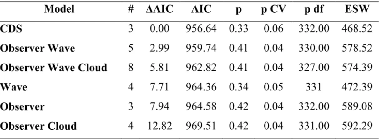
perpendicular distance data for minke whales (#: number of parameters; AIC: Akaike Information Criterion; p: average detection probability; ESW: effective strip width). 42 Table 5. Summary of model selection and parameter estimates for models proposed to fit

perpendicular distance data for fin whales (#: number of parameters; AIC: Akaike Information Criterion; p: average detection probability; ESW: effective strip width). 44 Table 6. Parameter estimates for the model that best fit fin whale perpendicular distance

data. ... 45 Table 7. Density and abundance estimates of baleen whales at the marine portion of the St.

Lawrence River Estuary (f(0): probability density function at zero distance; p: detection probability; ESW: effective strip width; DS: density of groups (number of groups km-2); D: density of whales (number of whales km-2); N: abundance estimate). ... 47 Table 8. Annual density and abundance estimates of baleen whales at the marine portion of

the St. Lawrence River Estuary (D: density of whales (number of whales km-2); N: abundance estimate). ... 48 Table 9. Definition of the spatial and environmental variables used to model baleen whales’

density in the marine portion of the SLRE. ... 67 Table 10. Total sightings of each baleen whale species available to fit the spatial density

model and the adopted values for detection probability ( pˆ ), effective strip width (w) and mean group size. ... 76

(14)

Table 11. Variance inflation factors for the environmental variables used to model baleen whales density within the SLRE. ... 80 Table 12. Spatial and environmental variables retained after model selection for each

baleen whale species. S indicates the use of a smooth function along with the degrees of freedom and transformation used (if any), both in parentheses. Percent of deviance explained and R2 adjusted for all models are also presented. * indicates significance level p-value of 0.001, **0.01. ... 100 Table 13. Estimated abundance (N) and density of groups (D) and the corresponding

coefficient of variation (CV%) derived from the spatial density models (SDM) and from conventional distance sampling (CDS) or multi-covariate distance sampling (MCDS) analysis. ... 101 Table 14. COSEWIC conservation status of each baleen whale species occurring in the

study area and weight adopted for the risk analysis. ... 120 Table 15. Categories adopted to represent the co-occurrence risk of whales and ships within

the study area... 122 Table 16. Adopted ethogram for the land-based observations of blue whales. ... 142 Table 17. Variables used to described blue whales’ breathing pattern and adopted

definitions ... 143 Table 18. Summary of Balaenoptera musculus’ breathing and movement parameters (±SD)

of the individual focal-follows conducted from two land-based stations located inside the Saguenay-St. Lawrence Marine Park in two consecutive feeding seasons (2008 and 2009) (μ : mean; DLB: distance to land-based station – mean (min;max); DCoast: distance to the nearest costline mean (min;max)). ... 147 Table 19. Adopted ethogram for the land-based observations of humpback whales. ... 172 Table 20. Total land-based tracking effective effort for each year and percentage kept to

characterize humpback whales’ exposure to whale watching activities at the peak of the touristic season within the Saguenay St. Lawrence Marine Park. ... 177 Table 21. Duration, period of the day (M: morning; A: afternoon; E: evening), exposure to

(15)

Neige, PP: Petit Prince, PS: Perseides, UK: unknown) of each individual focal follow retained to characterise humpback whale’ exposure to whale watching activities within the Saguenay St. Lawrence Marine Park (*split to compute exposure by period). ... 179 Table 22. Number of focal-follows conducted from each land-based station at the peak of

the touristic season within the Saguenay-St. Lawrence Marine Park in the presence and absence of each boat type. ... 181 Table 23. Humpback whales’ exposure to boats within a 1 km radius for each period of the

day at the peak of the touristic season within the Saguenay-St. Lawrence Marine Park. ... 181 Table 24. Mean, standard deviation (sd) and maximum (max) number of boats by distance

category recorded (for the main land-based stations and for all land-based stations combined) while tracking humpback whales at the peak of the touristic season within the Saguenay St. Lawrence Marine Park (* maximum of boats recorded at the same time within 100 m). ... 186 Table 25. Summary of the focal-follows of the humpback whale identified as Perseides

conducted within the Saguenay St. Lawrence Marine Park. (* focal-follows conducted after the 30th of July 2010 when a notification to avoid approaching the whale was emitted). ... 189 Table 26. Observation sites’ locations and bearing to reference object. ... xxxvi

(16)

Figures list

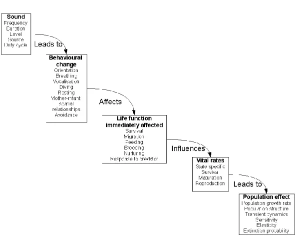
Figure 1. Conceptual model of the population consequences of acoustic disturbance on

marine mammals (National Research Council (NRC) 2005). ... 6

Figure 2. The study area overview showing its connection with the Gulf of St. Lawrence - one of the five ‘Large Oceanic Marine Areas (LOMA)’ identified by the Canadian government. ... 13

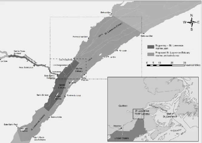
Figure 3. The marine portion of the proposed St. Lawrence Estuary Marine Protected Area (dot-dashed box) which constitutes the global study area and the marine portion of the Saguenay-St. Lawrence Marine Park (dashed box) where most of the data was collected. ... 14

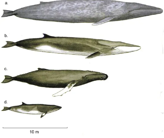
Figure 4. External morphology of the baleen whale species (a. blue whale; b. fin whale; c. humpback whale; d. minke whale) focus of the present study (Artwork: Daniel Grenier). ... 16

Figure 5. Surface feeding minke whale (Balaenoptera acutorostrata) (Photo: Chiara G. Bertulli/ORES). ... 18

Figure 6. Fin whales (Balaenoptera physalus) (Photo: Cris Albuquerque Martins). ... 20

Figure 7. Blue whale (Balaenoptera musculus) (Photo: Cris Albuquerque Martins). ... 22

Figure 8. Humpback whale (Megaptera novaeangliae) (Photo: Catherine Dubé). ... 24

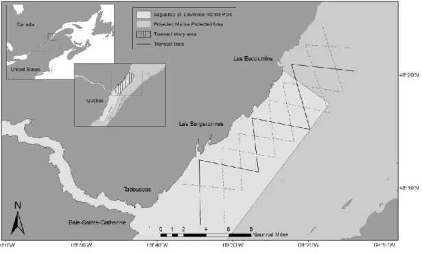
Figure 9. Transect lines designed for the systematic surveys conducted from 2006 to 2009. At each survey day a different set of lines (solid line, dashed line or dash-dot line) was monitored. ... 29

Figure 10. Transect lines completed during four years of systematic surveys conducted within the marine portion of the St. Lawrence River Estuary... 35

Figure 11. Location of the baleen whales recorded during the four years of systematic surveys conducted at the marine portion of the St. Lawrence River Estuary. ... 37

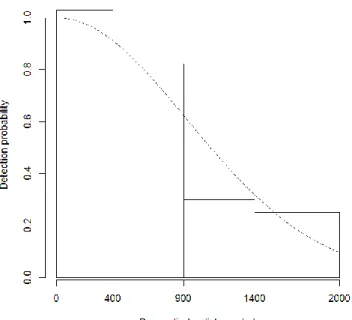
Figure 12. Histogram of recorded perpendicular distances of blue whales from the transect line and fitted detection curve (note that the x intervals are not equal). ... 38

(17)

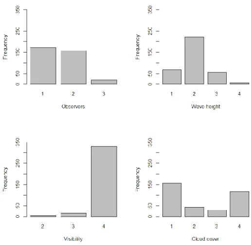
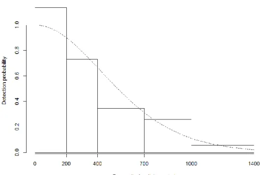
Figure 13. Histogram of recorded perpendicular distances of humpback whales from the transect line and fitted detection curve (note that the x intervals are not equal). ... 39 Figure 14. Distribution of variables available to model minke whales’ detection function. 40 Figure 15. Distribution of variables available to model fin whales’ detection function. ... 41 Figure 16. Histogram of recorded perpendicular distances of minke whales from the

transect line and fitted detection curve (note that the x intervals are not equal). ... 43 Figure 17. Histogram of perpendicular distances of fin whales from the transect line, fitted

detection curve (solid black line) and detection curves for each combination of wave height (dashed, dotted, and dot-dashed) and observer (gray, blue, red) (note that the x intervals are not equal). ... 45 Figure 18. Histogram of perpendicular distances of fin whales observed by wave height

level and corresponding fitted detection curve (note that the x intervals are not equal). ... 46 Figure 19. Annual abundance estimate of minke and fin whales (2006 to 2009) occurring

within the marine portion of the St. Lawrence River Estuary... 49 Figure 20. Annual abundance estimate of blue and humpback whales (2006 to 2009)

occurring within the marine portion of the St. Lawrence River Estuary. ... 50 Figure 21. Design used during systematic distance sampling surveys from 2006 to 2009 and

the proposed one that was adopted for 2010-2011 to ensure equal coverage probability (each day a different survey design (1, 2 or 3) was realized). ... 58 Figure 22. Example of design to estimate cetacean density and abundance while allowing

for equal coverage probability covering the whole marine portion of the St. Lawrence River Estuary (restricted to the area within the 40 m isobaths). ... 59 Figure 23. Area covered during line transect distance sampling surveys within the marine

portion of the St. Lawrence River Estuary. ... 65 Figure 24. Illustration of notation and of data preparation steps: the transect of length L was

subdivided in segments of length l (2 km), to which a central point was attributed and geographic coordinates, k environmental variables and the n recorded sightings (number of groups of each species) were associated (w is the effective strip width). . 66

(18)

Figure 25. Modeling framework to model the count data and predict the density of each baleen whale species within the study area. ... 70 Figure 26. Transect survey study area and grid established to predict baleen whales’ density

within the marine portion of the St. Lawrence River Estuary... 72 Figure 27. Grid adopted to extrapolate blue whales’ density within the marine portion of the

St. Lawrence River Estuary from Tadoussac to Betsiamites and delimited by the 50 m bathymetric contour. ... 75 Figure 28. Distribution of the survey effort (in minutes) in relation to the tidal cycle. ... 77 Figure 29. Distribution of the survey effort (from 0 to 1200 minutes) in relation to the tidal

cycle for survey days with at least one presence of each baleen whale species. ... 78 Figure 30. Distribution and correlation of the spatial and environmental variables used in

the spatial density model of baleen whales. ... 79 Figure 31. Bathymetry and slope within the marine portion of the St. Lawrence River

Estuary... 81 Figure 32. Zoom of the bathymetry within the marine portion of the Saguenay–St.

Lawrence Marine Park and indication of important topographic features. ... 82 Figure 33. Plots of the GAM smooth fits of the environmental covariates selected for minke

whales. Solid lines represent the best fit, the gray area represents the confidence limits, and vertical lines on the x-axis are the observed data values. ... 83 Figure 34. Surface map of minke whales predicted density of groups using generalized

additive models (above) and the coefficient of variation (CV) of the prediction (below). ... 84 Figure 35. Presence of spatial autocorrelation in the residuals, mainly at short distances (3 -

5 km), with the variogram of the residuals of minke whales’ prediction model and the Monte Carlo envelope. ... 85 Figure 36. Boxplot of the predicted density and abundance of minke whales derived from

(19)

Figure 37. Plots of the GAM smooth fits of the environmental covariates selected for fin whales. Solid lines represent the best fit, the gray area represents the confidence limits, and vertical lines on the x-axis are the observed data values. ... 87 Figure 38. Surface map of fin whales predicted density of groups using generalized additive

models (above) and the coefficient of variation (CV) of the prediction (below)... 88 Figure 39. Presence of a slight degree of spatial autocorrelation in the residuals with the

variogram of the residuals of fin whales’ prediction model and the Monte Carlo envelope. ... 89 Figure 40. Boxplot of the predicted density and abundance of fin whales derived from the

bootstrap. ... 90 Figure 41. Plots of the GAM smooth fits of the environmental covariates selected for blue

whales. Solid lines represent the best fit, the gray area represents the confidence limits, and vertical lines on the x-axis are the observed data values. ... 91 Figure 42. Surface map of blue whales predicted density of groups using generalized

additive models (above) and the coefficient of variation (CV) of the prediction (below). ... 92 Figure 43. Variogram of blue whales’ prediction model residuals’ and a Monte Carlo

envelope showing the absence of spatial autocorrelation in the residuals. ... 93 Figure 44. Boxplot of the predicted density and abundance of blue whales derived from the

bootstrap. ... 94 Figure 45. Surface map of the predicted density of blue whales derived from model-based

methods extrapolated to the marine portion of the SLRE, and its overlay with independent datasets... 95 Figure 46. Plots of the GAM smooth fits of the environmental covariates selected for

humpback whales. Solid lines represent the best fit, the gray area represents the confidence limits, and vertical lines on the x-axis are the observed data values. ... 96 Figure 47. Surface map of humpback whales predicted density of groups using generalized

additive models (above) and the coefficient of variation (CV) of the prediction (below). ... 97

(20)

Figure 48. Variogram of the residuals of the prediction model of humpback whales with the Monte Carlo envelope showing the absence of spatial autocorrelation in the residuals. ... 98 Figure 49. Boxplot of the predicted density and abundance of humpback whales derived

from the bootstrap. ... 99 Figure 50. Intensity of large ship traffic within the marine portion of the Saguenay - St.

Lawrence Marine Park (Adapted from Chion et al. 2009) and the current traffic separation scheme. ... 115 Figure 51. Fin whale strike in California - USA (Bernardo Alps/PHOTOCETUS). ... 117 Figure 52. Provisionary measures recommended by the working group on marine mammals

and maritime traffic (Groupe de travail sur le traffic maritime et les mammiferes marins G2T3M) to reduce collision risk within the St. Lawrence River Estuary. .... 118 Figure 53. Baleen whales’ spatial density models derived from line transect distance

sampling surveys conducted from 2006 to 2009 within the study area. ... 119 Figure 54. Characterisation of the degree of co-occurrence between baleen whale species

and large ship traffic within the study area. ... 124 Figure 55. Predicted degree of co-occurrence between the blue whale and the large ships’

traffic within the study area... 125 Figure 56. Overlay of the provisionary measures recommended by the working group on

marine mammals and maritime traffic (Groupe de travail sur le traffic maritime et les mammiferes marins G2T3M) and the characterisation of the degree of co-occurrence between baleen whale species and large ship traffic within the marine portion of the study area. ... 126 Figure 57. Overlay of the provisionary measures recommended by the working group on

marine mammals and maritime traffic (Groupe de travail sur le traffic maritime et les mammiferes marins G2T3M) and the characterisation of the degree of co-occurrence between baleen whale species and large ship traffic within the study area. ... 127 Figure 58. Overlay of the provisionary measures recommended by the working group on

(21)

mammiferes marins G2T3M), the degree of co-occurrence between baleen whale species’ (grouped and extrapolation model) and large ship traffic, and the traffic separation scheme of the St. Lawrence River Estuary. ... 128 Figure 59. Overlay of the co-occurrence risk map, the provisionary measures recommended

by the working group on marine mammals and maritime traffic (Groupe de travail sur le traffic maritime et les mammiferes marins G2T3M), the current navigation corridor and the proposed adjustment to reduce whale-boat co-occurence in the St. Lawrence River Estuary. ... 129 Figure 60. Overlay of the co-occurrence risk map and of the proposed adjustment to the

current traffic separation scheme avoiding high density areas and the 200 m bathymetric contour intended to reduce whale-boat co-occurrence in the St. Lawrence River Estuary. ... 130 Figure 61. Boundaries of the Saguenay – St. Marine Park, the proposed St. Lawrence

Estuary MPA and the land-based stations from which focal-animal observations of blue whales were conducted... 139 Figure 62. Individual blue whales’ tracks obtained from the land-based stations showing

fine-scale movement patterns (all valid fixes) within the northern shore one nautical mile zone. ... 146 Figure 63. Blow rate for each observed blue whale showing individual differences. Animals

exposed for longer periods showed a greater blow rate variance (0.73 - Spearman rho = 0.9, p < 0.05). ... 149 Figure 64. Simplified track (only true dive positions) of three focal animals showing

exposure to boats (presence within distance categories)and lack of compliance (boats within 400 m): a) individual followed the 5th September 2008 (050808A) from Bergeronnes (2.7 hours) – some surface periods without boats in between others in boats’ presence and with boats within 100 m in 5 surface intervals; b) individual followed the 20th August 2009 (200809J) from Mer et Monde (3.39 hours) – accompanied by boats during the whole observation period and with boats within 100 m in 10 surface intervals; c) individual followed the 20th August 2009 (200809H)

(22)

from Mer et Monde (2.6 hours) - accompanied by boats during the whole observation period and with boats within 100 m in 5 surface intervals. ... 151 Figure 65. General exposure of blue whales observed at the Saguenay–St. Lawrence Marine

Park by boat category and distance class. Compliant boats would be beyond 400 m of the focal animals. ... 152 Figure 66 Fine scale movement of blue whales and whale watching boats: a) “J” surface

geometry characteristic of foraging blue whales and a whale watching boat approaching it (050908A) using the forehead angle; b) another whale watching boat actively approaching the focal animal 200809H within 100 m and using the forehead angle; c) another active approach within 100 m of the focal animal (200809H). ... 155 Figure 67. The North Atlantic showing the principal feeding and breeding aggregations for

humpback whales (from Stevick et al. (2003)). ... 167 Figure 68. Boundaries of the Saguenay – St. Lawrence Marine Park, the proposed St.

Lawrence Estuary MPA and the land-based stations from which focal-animal observations of humpback whales were conducted. ... 171 Figure 69. Area surveyed during land-based data collection (1 km), distances adopted to

characterize exposure, and distances to be respected by the whale watching boats depending on boat type (commercial versus recreational boats). ... 175 Figure 70. Humpback whales’ tracks recorded from four land-based stations at the peak of

the touristic season from 2008 to 2010. ... 178 Figure 71. Humpback whales’ exposure (i.e. percent of time a whale has at least one boat

within a 1 km radius) for each period of the day at the peak of the touristic season within the Saguenay-St. Lawrence Marine Park (outliers are shown). ... 182 Figure 72. Periods throughout the day during which commercial zodiacs’ from each of the

three main ports within the Saguenay-St. Lawrence Marine Park can be engaged in whale watching activity according to the published schedule of each company operating in the area (assuming that at the peak of the season all offered trips take place). ... 183

(23)

Figure 73. Exposure of each individual focal-follow to commercial zodiacs, throughout the day at the peak of the touristic season at Saguenay-St. Lawrence Marine Park. ... 184 Figure 74. Average number of boats by distance category recorded (for all land-based

stations combined and the main land-based stations) while tracking humpback whales at the peak of the touristic season within the Saguenay St. Lawrence Marine Park. . 187 Figure 75. Maximum number of boats by distance category recorded (for all land-based

stations combined and the main land-based stations) while tracking humpback whales at the peak of the touristic season within the Saguenay St. Lawrence Marine Park. . 188 Figure 76. The humpback whale identified as Perseides observed from Mer et Monde in

2009 (above) and 2010 (below) illustrating the animal’s health conditions. The circles indicate the difference of blubber thickness in 2010. ... 190 Figure 77. Suggested speed reduction zone, baleen whales’ core areas and the provisionary

measures recommended by the working group on marine mammals and maritime traffic (Groupe de travail sur le traffic maritime et les mammiferes marins G2T3M). ... 206 Figure 78. The amazing experience of observing a humpback whale (Aramis) in the wild

(Photo: Cris Albuquerque Martins). ... 207 Figure 79. Suggested management measure to increase land-based and kayak whale

watching experience, enhance security and decrease whale exposure within an important core area. ... 208 Figure 80. Land-based whale watch of a blue whale from the Paradis Marin Camping

ground (Photo: Cris Albuquerque Martins). ... 209 Figure 81. Humpback whale (Petit prince) passing by a group of Kayaks in front of Mer et

Monde camping ground showing the usual configuration of kayaks accompanied by a guide (Photos: Pauline Gauffier). ... 209 Figure 82. Focal-follow (01/08/2010) of a humpback whale conducted from Mer et Monde

camping ground showing a high concentration of boats (zodiacs and kayaks) in the area and the lack of maneuverability for the whale (Photos: Pauline Gauffier). ... 211

(24)

Figure 83. Pilots boat approaching a container to go onboard and accompany it upstream the St. Lawrence River Estuary up to Quebec (Photo: Cris Albuquerque Martins). . 211 Figure 84. Spreadsheet used in the field during land-based station data collection. ... xxxiv Figure 85. Daily abstract spreadsheet used to have an overview of the data collected each

day. ... xxxv Figure 86. Errors associated with the measurements taken with a theodolite or total station

(Source: Würsig et al. (1991). ... lii Figure 87. Overlay of the measurements taken with the total station from the land-based

station at Les Bergeronnes and of the coordinates of the zodiac Astram recorded each second with a hand held GPS. ... liii Figure 88. Error of the measurements taken with the total station in relation to the

(25)

Acronym list

AIC: Akaike Information Criterion AIS: Automatic Identification System asl: above sea level

BR: Breathing rates

CDS: Conventional Distance Sampling CV: coefficient of variance

D: density of individuals df: degrees of freedom DS: density of groups

DBM: Design based methods

DFO: Department of Fisheries and Oceans ESW: Effective strip width

FF: Focal-follow

FHAMIS: Fisheries Habitat Management Information System GAM: Generalized Additive Model

GCV: General Cross Validation score GIS: Geographic Information System GOF: Goodness of Fit test

GPS: Global Positioning System

GREMM: Groupe de Recherche et Éducation sur les mammifères marins GSL: Gulf of St. Lawrence

IFAW: International Fund for Animal Welfare IUCN: International Union for Animal Welfare IWC: International Whaling Commission LBWW: Land-based whale watching LCH: Laurentian Channel head LOMA: Large Oceanic Marine Area

(26)

MBM: Model based methods

MCDS: Multiple-covariate Distance Sampling MICS: Mingan Island Cetacean Study

MM: Mer et Monde

MPA: Marine Protected Area N: abundance

SARA: Canadian Species at Risk Act SD: Standard deviation

SDM: Spatial density model SES: Socio-ecological system SLRE: St. Lawrence River Estuary

SSLMP: Saguenay St. Lawrence Marine Park TSS: Traffic separation scheme

VIF: variation inflation factor

(27)

À todos os filhos. E aos filhos dos filhos. E filhos dos filhos…dos filhos….dos filhos. Filhos da mãe Terra. Filhos que seguem na busca por uma vida plena e em harmonia com todos of filhos dos filhos de todos os seres do Universo.

A tous les fils. Et aux fils des fils. Et les fils des fils...des fils...des fils. Fils de la mère Terre. Fils qui sont á la recherche d’une vie pleine et en harmonie avec tous les fils de tous les êtres de l’Univers.

(28)

Acknowledgements

Many people have contributed in some way to this stage of my life. Some have contributed to the begin of this journey, others were always present giving me the solid base I needed to keep on going, some have joined my path and are now following their own paths, and a special one joined my path to improve it, bringing colour and warming it.

My family, specially my mother, deserves most of the credit for it. Without their love and support I would never be able to accomplish it. Obrigada mãe! Obrigada por tudo! Thanks Lu, Rafa, Biel! Even the distance between the south and the north cannot create a distance among us. Pai, o processo foi longo, mas foi cheio de aprendizado e com certeza me fara chegar ao pote de ouro! Meu querido anjo Mikaël, espero com esse trabalho poder contribuir pra que a sua geração e as vindouras possam disfrutar de um Planeta tão biodiverso ou mais que o que temos agora!

Dr. Lael Parrott, thanks for giving me the chance to discover this unique ecosystem, co-managed by authorities of Quebec and Canada. Thanks for introducing me to the Complex Systems universe! I hope soon we will have enough base knowledge on cetacean’s ecology to build bottom-up models that might improve our understanding of their ecology. Thanks for your wisdom, trust, your enthusiasm with the project, encouragement and support of all kinds! I learnt a lot with you!

Robert Michaud, president of the Groupe de Recherche et Éducation sur les Mammifères Marins (GREMM), provided me with an unique opportunity to analyze the data from the systematic surveys conducted by his organization allowing me to learn a lot and to provide a real contribution to the knowledge of this amazing ecosystem. It was an amazing experience to dive in the ecology of a whales’ feeding ground. I learnt a lot and I appreciate your support and guidance throughout all this process. I hope my work will in some way contribute to the important work you and the organization you represent conduct to the marine mammal conservation in the area.

(29)

An important part of the data analyzed in this thesis was collected by the GREMM with the financial support of the Saguenay-St. Lawrence Marine Park and Fisheries and Oceans Canada. Marie-Helene Darcy, Renaud Pintiaux, Guillaume Pelletier and Sarah Duquette were responsible for most of the data collection and data entry. A special thanks to Michel Moisan, who was responsible for observers’ training, data collection protocol, data entry, data transformation, data share, data correction, data extraction, data, data…Thanks a lot!!!! Thanks to Patrice Corbeil for all technical support, Véronik de la Chenelière (for all support, and for your inspiring house) and all the gremmelins I had the pleasure to meet during this period.

The land-based field work was funded by the Natural Sciences and Engineering Research Council of Canada (NSERC) as part of a Strategic Grant awarded to Dr. Lael Parrott. Its success relies on many people. Kate Hawkes, Mark Chikhani and France Morneau were research assistants during the pilot study and first year of data collection. Ambra Blasi, Pauline Gauffier, Jamie Raper, Natalia Mamede, Mouna Petitjean, Maita Lisboa de Moura and Breena Apgar-Kurtz were volunteers during the second and third year of data collection. A special thanks to Ambra and Kate, for their friendship and all the help with data organisation and cleaning. Maria E. Morete, who taught me how to conduct land-based studies and showed me how amazing is to observe whales with the right eye! Besides, she came twice from Brazil to help me out during data collection. I would like to thanks Manuela Conversano for her friendship and her help with field-work logistics and to put me in contact with Bernard Tessier (Fisheries and Oceans Canada), who was responsible for the total station loan in 2009 and 2010. Claudine Boyer (Canada Research Chair in Fluvial Dynamics) for equipment loans and technical support with the DGPS. Pierre Hersberger (Mer et Monde écotours) for kindly allowing me to set one of the land-based stations at the best spot of his camping ground! To all the friends from the Ècole de la Mer who kindly received us at their home during the field work of 2009 and 2010!

A special thanks to Samuel Turgeon who built the land-based database and developed an important part of the land-based data treatment protocol. As a research

(30)

assistant of the Complex System Laboratory, he contributed in different stages of the data processing. In addition, he actively participated of the spatial density modelling analysis, and provided valuable comments and insights that improved the thesis. His friendship became love, and his support was essential for the completion of this work. Merci mon amour!

Danielle Marceau (University of Calgary), Guy Cantin (Fisheries and Oceans Canada), Jacques-André Landry (École de Technologie Supérieure), Marc Mazerolle (CEF), Nadia Ménard (Parks Canada Agency), Pierre André (UdeM), Suzan Dionne (Parks Canada Agency) provided valuable insights that guided the definition of the research project and/or valuable comments on the written version of it. Fréderic Delland, Benoit Dubeau and Valérie Busque from Parks Canada for support during the fieldwork, calibration of the land-based station and literature updates concerning the Marine Park, respectively. Veronique Lésage (Fisheries and Oceans Canada) and Dany Zbinden (Mériscope Marine Science Centre) provided valuable data to validate the spatial model.

Je remercie la Faculté des études supérieures (FES) de l’Université de Montréal pour l’attribution de deux bouses d’exemption des droits de scolarité supplémentaires, ainsi qu’au département de Géographie pour les bourses accordées entre 2007 et 2011. Je remercie également Dr. Parrott pour l’attribution des bourses d’étude entre 2007-2009, dans le cadre du projet stratégique financé par le Conseil de recherches en sciences naturelles et en génie du Canada (CRSNG) en collaboration avec Parcs Canada, Pêche et Océans, le GREMM, l'École de technologie supérieure (Montréal) et l'Université de Calgary. Je remercie tout le personnel du département de Géographie pour avoir rendu mon parcours académique plus agréable et sans obstacle, en particulier Linda Lamarre, Lolita Frechette, Sylvie Beaudoin, Susy Daigle, Anne-Marie Dupuis, Isabelle Pelletier, Sophie Labelle, Nathalie Désilets, Marc Girard, Richard et Claude! Pour son amitié ainsi que pour le support informatique essentiel, un énorme merci à Gilles Costisella!

(31)

Évidemment que mes années à Montréal ont été´beaucoup facilitées par les bons amis que j’ai rencontré (Raquel, Fred, Ana, Karime e Gustavo, vocês também fazem parte da gang! Gracias Luis!) surtout au département de géographie et au Laboratoire sur les systèmes complexes! Rodolphe Gonzales mon ami avec la main verte (ou rouge…), Patrick Verhaar, Dago Hacevedo, Christine Grenier, Elise Filotas, Raphael Proulx, Guillaume Latombe, Caroline von Schilling, Caroline Gaudreau, Samuel Turgeon, Philippe Lamontagne, Clément Chion, Rémi Labrecque, and all the others that I will not list here to save a tree!

Aos meus amigos queridos do Brasil, que mesmo longe estão sempre perto! Nossa amizade nutre minha alma!! Um obrigada especial ao Andrey Piovezan, a Luciana Guidoux e a Erika de Almeida!

(32)

Chapter 1

(33)

1.1 Introduction

Records of human-whale interactions date to ancient times. The first records of whale hunting date from 1000 B.C., by Phoenicians in the Mediterranean Sea (Reeves et al. 2002). Since this time, our relation with marine mammal species has passed through different phases. Marine mammals have inspired the development of myths (mermaid), furnished oil for lighting and skin for clothing. After a period of intensive hunting, in modern days, they constitute a conservation symbol, used as sentinel, umbrella, or flag species in different parts of the planet (Aguirre and Tabor 2004; Bonde et al. 2004). Despite this, the increasing development of human societies still poses many treats to the environment in which cetacean species have evolved.

Nowadays, human societies occupy all the biomes (Ellis and Ramankutty 2008) and the coastal zone is amongst the most modified areas (Bollmann et al. 2010). A total of 755 of the mega-cities with populations over ten million are located in the coastal zones and 90% of the fisheries occur in coastal waters (Bollmann et al. 2010). As the human footprint enlarges, humanity is challenged to develop and deploy understanding of large scale commons governance to ensure sustainability (Dietz et al. 2003).

Successful adaptive strategies for ecosystem management include 1) building knowledge and understanding of resource and ecosystem dynamics, 2) developing practices that interpret and respond to ecological feedback, and 3) supporting flexible institutions and organisations and adaptive management processes (Berkes and Folkes 1998; Olsson et al. 2004). The present work aims to support the adaptive management of the St. Lawrence River Estuary (SLRE) ecosystem and particularly the conservation of baleen whale species in that system, by addressing points (1) and (3).

The SLRE is a complex socio-ecological system (SES). By definition a SES is an ecological system intricately linked with and affected by one or more social systems (Gallopin et al. 1988; Shaw et al. 1992). The SLRE is a rich ecosystem, a millenary habitat for different marine mammal species and a place where many social systems have evolved. Among the social systems that are intricately linked with the marine mammals in the

(34)

SLRE, two are of essential importance: the maritime traffic and the whale watching (WW) industry. Even if these social systems are quite different they use the SLRE for navigation purposes and their activities pose similar threats to cetacean species.

Noise pollution and collision risk are direct consequences of high levels of maritime traffic. Noise pollution can trigger short-term responses and can have long-term consequences for cetacean species (Richardson et al. 1995; Weilgart 2007). Short-term response may trigger serious population consequences or they may be insignificant, and on the other hand, long-term impacts may occur in the absence of observable short-term reactions (Weilgart 2007). In addition, the impact of noise pollution may be magnified when individuals show high site fidelity (Corkeron 2004; Bejder et al. 2006; Lusseau and Bejder 2007; Schaffar et al. 2010). In its turn, ship strikes can jeopardise the viability of small populations of cetacean (Fujiwara and Caswell 2001).

1.1.1 Maritime traffic effects on cetacean species

Reactions to boats are mainly a reaction to the sound they produce. Sound is a compression wave that causes particles of matter to vibrate as it transfers from one to the next (Hatch and Wright 2007). Speed of sound in seawater is the same for all frequencies, but varies with aspects of the local marine environment such as density, temperature, and salinity. The latter is of high importance in estuarine ecosystems (Hatch and Wright 2007). Depth and substrate characteristics have also an important role in sound propagation.

Marine mammals have evolved to use sound as a means of communicating, finding prey and sensing their environment. They are even capable of long-distance communication by using the oceanographic characteristics of the ocean. The sound channel (SOFAR channel), as it is called, occurs at a depth of about 800-1000 m at mid-latitudes. But its depth varies from over 1600 m in the warmest waters of the world to 100 m in colder waters and can even reach the surface at the ice edge, becoming a surface sound channel that allows long-distance communication among animals (Hatch and Wright 2007). In feeding areas, long distance communication might have an important role for baleen whales. As the food resource is patchily distributed, communicating a found patch to

(35)

conspecifics might benefit the population on a long-term basis (R. Sousa-Lima, personal communication).

However, the amount of human-related sound in the oceans has increased over a very short time frame in evolutionary terms, providing only a few generations for species to adapt (Hatch and Wright 2007). With seismic surveys and naval exercises, marine traffic is among the three main sources of noise production at sea (Richardson et al. 1995). The increase of propeller-driver vessels has caused a rise of low-frequency ambient noise of approximately 3 dB/decade over the past 50 years (Hatch and Wright 2007).

Noise is a ubiquitous stimulus with the potential to act as a stressor (Wright et al. 2007). Boat noise can affect cetacean species in different manners: it can mask important sounds, induce vocal behaviour change, cause hearing loss, and confound animal’s decision-making besides having cumulative physiological effects (Richardson et al. 1995; Bateson 2007; Weilgart 2007). This could happen through interference with their ability to detect calls from conspecifics, echolocation pulses, or other important natural sounds (Richardson et al. 1995). Reactions can range from brief interruptions of normal activities to short or long-term displacements from noisy areas. Previous research indicates that gray (Eschrichtius robustus), humpback (Megaptera novaeagliae) and bowhead (Balaena misticetus) whales may have reduced their utilization of certain heavily disturbed areas (Richardson et al. 1995), and that they moved away from preferred feeding areas when disturbed by vessels (Baker and Herman 1989; Borggaard et al. 1999).

Mysticetes species, which include all the whales focused on in this study, produce and have ears well adapted to receive low frequency sounds (Croll et al. 2001). Low-frequency vessel noise often masks fin whale (Balaenoptera physalus) social sounds, and higher-frequency outboard noise masks minke whale (Balaenoptera acutorostrata) sounds (Richardson et al. 1995). Studies of the songs of humpback whales approached by boats indicate that the durations of some song elements are altered (Norris 1994; Sousa-Lima et al. 2002) and that the vocal behaviour could be interrupted (Tyack 1981). The consequences of this disruption on individuals and the population are poorly understood. It may result in disruption of social ordering, sexual behaviour, care of the young and of

(36)

cooperative activities (Richardson et al. 1995). In an Alaskan feeding ground, it was detected an increase in the rate and repetitiveness of sequential use of feeding call types by humpback whales associated with noisy areas (Doyle et al. 2008). Furthermore, strong sounds might cause temporary or permanent reductions in hearing sensitivity (Richardson et al. 1995). Also, a noisy environment can affect animal decision-making by masking the incoming information completely, partially or rendering it ambiguous. Besides, it can generate an emotional state of fear or anxiety, which could change their decision-making and increase collision risk (Bateson 2007).

To date, much still needs to be done in order to understand the degree to which human activities (such as anthropogenic noise) induce physiological and behavioural responses, which ultimately could result in changes of population dynamics such as reduced yearly survival and fecundity (Wintle 2007). However, we are beginning to realise that non-lethal impacts of human disturbance can also have serious conservation implications (Wright et al. 2007) . Possibly the most important of non-lethal impacts arises from the prolonged or repeated activation of the stress response, and its likelihood to induce chronic stress. Chronic stress is linked to numerous conditions in humans, including coronary disease, immune suppression, anxiety and depression, cognitive and learning difficulties, and infertility (Wright et al. 2007). The conceptual model developed by the US National Research Council (2005) provides a complete overview linking sound to short-term effects at the individual level that could result in long-short-term effects at the population level (Figure 1).

Besides the secondary effects of noise pollution, marine traffic brings with it an intrinsic collision risk (Richardson et al. 1995). These factors may explain, at least in part, why some species have not recovered after protective measures have been put into place (Wright et al. 2007), as in the case of the St. Lawrence River Estuary beluga whale (Delphinapterus leucas) population, which does not show signs of recovery in the last 20 years (MPO 2011).

(37)

Figure 1. Conceptual model of the population consequences of acoustic disturbance on marine mammals (National Research Council (NRC) 2005).

In recent years, a great effort to measure the impact of large ship traffic on cetacean species is ongoing (IWC 2009). However, most collision events are still unreported. Ritter (2009) made a first search for collision events with sailing vessels by using an Internet form. A total of 81 collisions and 42 near misses were reported, spanning from 1966 until 2008 and from different parts of the world. Vessel type and speed as well as circumstances of the incident varied widely, but most often monohulls were involved, predominantly sailing at speeds between 5 and 10 knots. Most reports referred to “large whales”. Trends involving other boat types are not yet available.

Among the eleven species known to be hit by large ships, fin whales are struck most frequently; right whales (Eubalaena glacialis and E. australis), humpback whales, sperm whales, and gray whales are hit commonly (Laist et al. 2001). In some areas, one-third of

(38)

all fin and right whale strandings appear to involve ship strikes. Lethal or severe injuries are caused by ships 80 m or longer since whales usually are not seen beforehand or are seen too late to be avoided and most lethal or severe injuries involve ships travelling 14 knots or faster (Laist et al. 2001). It was demonstrated that the greatest rate of change in the probability of a lethal injury to a large whale occurs between vessel speeds of 8.6 and 15 knots where the probability of a lethal ship strike increases from 0.21 to 0.79 (Vanderlaan and Taggart 2007).

Most ship strikes reported with cetaceans occurred in the North Atlantic (Laist et al. 2001; Van Waerebeek and Leaper 2008; Ritter 2012). Panigada et al. (2006a) review ship collision records for the relatively isolated population of fin whales in the Mediterranean Sea from 1972 to 2001. Out of 287 carcasses, 46 individuals (16.0%) were certainly killed by boats. The minimum mean annual fatal collision rate increased from 1 to 1.7 whales/year from the 1970s to the 1990s. Fatal strike events (82.2%) were reported in or adjacent to the Pelagos Sanctuary, an area characterized by high levels of traffic and whale concentrations. Besides, among 383 photo-identified whales, 9 (2.4%) had marks that were attributed to a ship impact. In the St. Lawrence, many whales present such marks, although the exact proportion of affected animals is unknown. Among the blue whales photo-identified in the Gulf of Saint Lawrence (GSL), 16% bear scars that were likely to be caused by collisions with vessels (Ramp et al. 2006).

Local measures to mitigate ship strike have been suggested and/or have been undertaken in different places. The reduction of collision risk between commercial ships and the North Atlantic right whales have be the focus of a multi-lateral effort, which involved in depth data analysis, real time monitoring of whales and boat trajectories and the modification of shipping routes (Kraus et al. 2005; Merrick and Cole 2007; Vanderlaan et al. 2008). At the Pelagos Sanctuary, many studies suggest the use of real-time monitoring of whale presence to inform management strategies such as the modification of ferry routes and/or speed reductions due to high co-occurrence rates, mainly with fin whales (Panigada et al. 2006b; David et al. 2011). Modification of shipping lanes was suggested as a measure to improve humpback whale protection on their Brazilian breeding ground (Martins 2004)

(39)

and in Panama (IWC 2012). At the Glacier Bay National Park and Reserve (Alaska), speed reductions were suggested as an effective measure to reduce collision risk and a temporary speed limit of 13 knots during the humpback whale occurrence season was adopted (IWC 2007; Harris et al. 2012). The same speed limit was adopted in the Strait of Gibraltar from 2007 on, and a lane modification was also implemented (IWC 2007). To date, boats transiting within the SLRE have their speed limited to 25 knots while crossing the Saguenay–St. Lawrence Marine Park (SSLMP), and boats engaged in whale watching activities should limit their speed to 10 knots while inside an observation zone / area (SOR/2002-76).

As large boats pass through an area of great importance for cetacean conservation, their speed matters not only due to the risk of collision, but also due to the almost positive correlation between ship speed and noise production. The participants of the “Global Scientific Workshop on Spatio-temporal Management of Noise” (Agardy et al. 2007) agreed that measures to create spatio-temporal restrictions of noise, also as part of Marine Protected Areas (MPAs) management plans, offer one of the most effective means to protect cetaceans and their habitat from the cumulative and synergistic effects of noise (Weilgart 2007). Indeed, including noise in marine spatial planning requires knowledge of noise levels on large spatial scales. Erbe et al. (2012) developed a simple tool based on Automatic Identification System (AIS) data to derive large-scale noise maps that allow the development of management strategies to keep quiet areas quiet and of mitigation measures to make noisy areas quieter.

Although large ships traffic and whale watching activities can induce similar effects on cetacean species, conservation measures to reduce the impact of the later are not as straightforward. Speed reduction as a measure to reduce collision risk and noise production can be applied to all kinds of boats. However, as whale watching activities are directed towards cetacean species, measures to minimise its effects have to include general and specific measures. The specific measures depend on the target species, their main activity in the area, and the characteristics of the industry that targets them, among others.

(40)

Besides the effects of noise production and collision risk exposed above, whale watching activities can also induce changes in movement pattern, respiratory behaviour, and even cause distribution shifts. Modification of movement parameters and breathing rates are usually concomitant. By using multiple linear regression analysis it was observed that humpback whales breeding at New Caledonia significantly increased their dive time from 2.7 (±2.4) to 3.1 min (±1.9), and decreased the linearity of their path when boats were present within 1000 m of the animals. The effect on linearity also proved to increase with the number of boats (Schaffar et al. 2010). Similar results have been reported for humpback whales in other breeding areas (Scheidat et al. 2004; Morete et al. 2007), for orcas (Bain et al. 2006), and sperm whales (Physeter macrocephalus) (Richter et al. 2006), to list a few. While changes in movement and breathing pattern are a short-term behavioural impact, it is also likely to increase energetic costs, which could have longer-term conservation implications (Lynas 1994; Constantine et al. 2004; Scheidat et al. 2004; Bejder et al. 2006; Boye et al. 2010; Schaffar et al. 2010; Visser et al. 2010; Steckenreuter et al. 2011).

1.1.2 Large ship traffic and whale watching activities within the SLRE

The SLRE is the main navigation entry of the eastern Canadian Coast. Large ship traffic within the SLRE is intense and might double in the coming years (Ircha 2005). The only information to date to characterize the maritime traffic is restricted to the SSLMP. Chion and colleagues (2009) provided the first comprehensive characterization of the maritime traffic within the SSLMP for the year of 2007.

In order to characterize the commercial ships traffic, Chion et al. (2009) used AIS data and prevision data from the Information System on Marine Navigation (INNAV) of the Canadian Coast Guard. A total of 3135 transits were made within the SSLMP from May to October 2007 by more than 650 different ships (i.e. cargo ships, tankers and tug/tows). The number of transits showed little fluctuation along the period (fortnights and week days) and throughout the day. However, a 9% increase in the number of transits was observed from 2003 to 2007. A similar volume of traffic was found within the Gerry E. Studds Stellwagen Bank National Marine Sanctuary in 2006 (Hatch et al. 2008). They

(41)

registered 541 large commercial vessels and a total of 3413 transits within the Marine Sanctuary for that year.

Besides large commercial ships, Chion and colleagues (2009) also provides a complete description of the other boat types that use the area. The higher number of transits within the studied period (22 541 transits) was attributed to the ferry boats that link the villages of Baie-Sainte-Catherine and Tadoussac, at the mouth of the Saguenay River. The second component of the maritime traffic in terms of number of transits is the whale watching industry (WW). In 2007, they estimated that 13 073 excursions took place between May and October 31st.

The first WW expedition in the SLRE took place in 1971. It was organized in collaboration with the Montreal Zoological Society, used occasional charters and amounted to no more than two per year (Lynas 1990). The activity followed its natural evolution from there and in 1988, 11 whale watching boats were operating regularly in the area. At this time, the industry’s gross income was estimated as 11.6 million (Lynas 1990).

Concern about the WW industry’s impact on whales was already discussed in 1988, always with a greater focus on beluga whales due to the species’ reduced numbers and annual occurrence. At that time, a call for a regulatory policy was proposed as a precautionary measure (Lynas 1990). The adoption of the Marine Activities Regulations in 2002 was an important step towards species’ protection and the sustainability of WW activities. In addition, the number of boats operating under permit to practice commercial observation activities at sea inside the Marine Park was limited to a maximum of 59 as of 2003 and has remained relatively constant, although a few permits have become inactive. As for the number of excursions per day, there is a small demand for early morning excursions, but overall, the number of excursions has remained relatively constant over the years (N. Ménard, personal communication). However, the lack of commitment to the current regulation and of an effective monitoring system diminishes its effectiveness.