HAL Id: hal-00945199
https://hal.inria.fr/hal-00945199
Submitted on 25 Mar 2014HAL is a multi-disciplinary open access archive for the deposit and dissemination of sci-entific research documents, whether they are pub-lished or not. The documents may come from teaching and research institutions in France or abroad, or from public or private research centers.
L’archive ouverte pluridisciplinaire HAL, est destinée au dépôt et à la diffusion de documents scientifiques de niveau recherche, publiés ou non, émanant des établissements d’enseignement et de recherche français ou étrangers, des laboratoires publics ou privés.
Jean-Loic Le Carrou, François Gautier, Roland Badeau
To cite this version:
Jean-Loic Le Carrou, François Gautier, Roland Badeau. Sympathetic string modes in the concert harp. Acta Acustica united with Acustica, Hirzel Verlag, 2009, 95 (4), pp.744–752. �hal-00945199�
Jean-Lo¨ıc Le Carrou and Fran¸cois Gautier∗ LAUM, CNRS, Universit´e du Maine, Av. O. Messiaen, 72085 LE MANS, France
Roland Badeau
T´el´ecom Paris (ENST) / CNRS LTCI, 46 rue Barrault, 75634 Paris Cedex 13, France
Abstract
The concert harp is composed of a soundboard, a cavity with sound holes and 47 strings. When
one string is plucked, other strings are excited and induce a characteristic ‘halo of sound’. This
phenomenon, called sympathetic vibrations is due to a coupling between strings via the instrument’s
body. These sympathetic modes generate the presence of multiple spectral components in each
partial of the tone. Resolution of Fourier analysis does not permit their identification. A high
resolution Method, called ESPRIT, is used to separate the spectral components which are very close
one to another. Some of the measured spectral components in the analysed partials correspond
to the response of sympathetic modes. The eigenfrequencies and mode shapes of these modes
are investigated using a suitable model of the instrument : this model is based on a waveguide
approach in which bending and longitudinal motions of 35 strings connected to an equivalent beam
representing the soundboard are described. Identified experimental sympathetic modes are very
well captured by the model.
PACS numbers: 43.75.Gh
I. INTRODUCTION
The harp is probably one of the oldest string instruments whose origin goes back to the Prehistory where the first men were charmed by the sound produced by their bow’s string. This chordophone was first composed of a few strings attached on an arched frame on one side and on a soundboard on the other side. Then, with the increase of the number of strings, a pillar was added between the neck and the soundboard to support the strings’ tension. This kind of harp was particularly used in Europe and marks the origin of the current concert harp. Nowadays, the concert harp is composed of 47 strings, from Cb0 (of fundamental frequency 30.9 Hz) to Gb7 (of fundamental frequency 2960 Hz), attached to the soundboard though an eyelet below which they are knotted. The soundboard is designed to withstand the stress imposed by the strings, as for the Camac concert harp used in this study, which is composed of multiple layers of different materials (aluminium, carbon, woods). From an acoustical point of view, the role of the soundboard is to radiate the sound produced by the vibrations of the strings. To some extent, this sound can also be amplified by the soundbox and its five sound holes [1]. In spite of mechanical and constructional improvements, musicians and harp makers alike are annoyed by the feeling produced by the halo of sound when the instrument is played. Indeed, when one string is plucked, in some tuning configurations some others are also excited by sympathetic vibrations. Although this phenomenon is a fundamental characteristic of the instrument’s
sound, the instrument maker has to design the harp so that sympathetic vibrations remain reasonable.
The sympathetic couplings between strings lead to phenomena of aftersound and some-times to beats. These phenomena are due to the fact that some partials of the sound may contain several spectral components whose frequencies are very close one to another. Two kinds of couplings are involved in this situation: couplings between different polarizations of a same string due to the way it is fixed and sympathetic couplings between different strings via the instrument’s body [2].
Considering the connection point between a single string and the soundboard as a point, the string/structure interaction can be described by a 6 by 6 admittance matrix. In such a description, three translational degrees of freedom and three rotational degrees of freedom are involved [3]. As a consequence, for one single string, each mode can have up to 6 components, their frequencies being very close one to another in the string’s response. However, in practice, 2 components often overshadow the others and correspond to 2 polarizations of the string. This has been shown for the guitar [4]. The strong anisotropy of the string/structure interaction (for the out-of-plane and in-plane directions) is responsible for this effect. As a consequence, the decay rates of the two polarizations of a single string are generally different and lead to a double decay effect [2].
The case of piano strings, which are grouped in pairs or triplet has often served as a framework for the study of sympathetic couplings. These couplings occur because each group of strings (pair or triplet) is practically tuned in unison. The case of two strings tuned in unison having the same polarization, coupled by a bridge motion is studied in [2]: normal modes for this configuration appear in pairs and depend on the strings mistuning and bridge admittance. It is the presence of these two coupled modes that is responsible for phenomena of beats and aftersound. The more complex case of a pair of piano strings tuned in unison, each of them having two polarizations has been studied in [5].
Similar coupling mechanisms exist in string instruments which do not have pairs of strings tuned in unison. This has been illustrated for the American five-string banjo: in [6], this instrument is modelized by an assembly of one-dimensional sub-systems in which waves propagation occur, allowing the time-domain response to be computed. It is shown that when all the strings are incorporated to the model, the decay time is shorter than when only one string is considered. This is explained by the presence of sympathetically driven strings, even if it is difficult to find out how sympathetic vibrations occur with this model.
For the kantele, which is a Finnish plucked five-string instrument, sympathetic vibrations are also identified in [7]. Through the experimental analysis of the total amount of energy transferred from one string to all the others, it can be shown that the transfer of energy is more pronounced between strings which have simple harmonic relationships.
In a previous paper [8], it has been shown that the sympathetic phenomenon is due to the presence of particular modes, called sympathetic modes, in the modal basis of the system. These modes have been both theoretically and experimentally identified on a simple academic configuration close to the harp: two strings tuned to the octave and connected to a beam were considered and the modes of this assembly were investigated. The aim of the present paper is to identify the sympathetic modes in the response of a real concert harp.
In the first part, an adequate experimental setup and an analysis based on a ‘High Reso-lution’ method are carried out to identify frequency components present in one partial when one string is plucked. Note that ‘High Resolution’ techniques are suitable for the spectral analysis of signals having very close spectral components, which cannot be separated using a Fourier analysis because of a lack of resolution. In the second part, the sympathetic vibra-tions are investigated through the use of a physical model of a simplified concert harp. In the final part, a comparison between theoretical and experimental results give an explanation of the origin of the sympathetic phenomenon in the instrument.
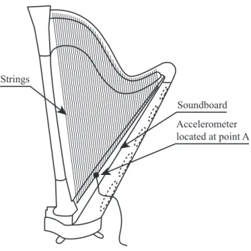
Strings
Soundboard Accelerometer located at point A
FIG. 1: Schematical representation of the experimental setup.
II. EXPERIMENTAL INVESTIGATION OF THE HARP’S SYMPATHETIC
MODES
A. Experimental setup
In order to experimentally highlight the presence of sympathetic modes in the concert harp, the following experimental protocol has been set up: the harp is plucked whereas an accelerometer is used to measure the vibratory signal on the soundboard at point A, as shown in Figure 1. This point is located on the inner surface of the soundboard, between the
Db3-string and the Cb3-string, respectively labelled 30 and 31. The played string is string 31
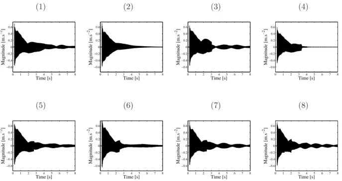
and the other strings are either damped or stopped during oscillations. Eight experimental configurations presented in Table I have been defined to investigate the characteristics of
TABLE I: Characteristics of the experimental configurations. String 24 corresponds to Cb2 of
fundamental frequency 246.9 Hz, string 31 to Cb3 (123.5 Hz), string 35 to Fb3 (82.4 Hz), string 38
to Cb2 (61.7 Hz) and string 42 to Fb1 (41.2 Hz).
Configuration Description
(1) All strings free to vibrate
(2) All strings damped except string 31
(3) String 31 stopped during oscillations
(4) Strings 24, 31, 35, 38 and 42 stopped during oscillations
(5) Strings 31 and 24 stopped during oscillations
(6) Strings 31 and 35 stopped during oscillations
(7) Strings 31 and 38 stopped during oscillations
(8) String 31 and 42 stopped during oscillations
sympathetic vibrations.
All measured signals are sampled to 4096 Hz and last 8 seconds. The string is stopped by the harp player a few seconds after the plucking of string 31. The temporal signals measured following the eight configurations are shown in Figure 2. These signals highlight a fact well-known by the harpists: the stopping of a string plucked does not necessarily imply a fast decrease of the sound level. Indeed, as shown in configurations (3), (5), (6), (7) and (8), the end signal amplitude is of the same order of magnitude that in the free-strings
(1) (2) (3) (4) 0 1 2 3 4 5 6 7 8 −0.6 −0.4 −0.2 0 0.2 0.4 0.6 Time [s] Magnitude [m.s −2 ] 0 1 2 3 4 5 6 7 8 −0.6 −0.4 −0.2 0 0.2 0.4 0.6 Time [s] Magnitude [m.s −2 ] 0 1 2 3 4 5 6 7 8 −0.6 −0.4 −0.2 0 0.2 0.4 0.6 Time [s] Magnitude [m.s −2 ] 0 1 2 3 4 5 6 7 8 −0.6 −0.4 −0.2 0 0.2 0.4 0.6 Time [s] Magnitude [m.s −2 ] (5) (6) (7) (8) 0 1 2 3 4 5 6 7 8 −0.6 −0.4 −0.2 0 0.2 0.4 0.6 Time [s] Magnitude [m.s −2] 0 1 2 3 4 5 6 7 8 −0.6 −0.4 −0.2 0 0.2 0.4 0.6 Time [s] Magnitude [m.s −2] 0 1 2 3 4 5 6 7 8 −0.6 −0.4 −0.2 0 0.2 0.4 0.6 Time [s] Magnitude [m.s −2] 0 1 2 3 4 5 6 7 8 −0.6 −0.4 −0.2 0 0.2 0.4 0.6 Time [s] Magnitude [m.s −2]
FIG. 2: Accelerometer signals measured at point A for the eight experimental configurations defined
in Table I. 200 0 400 600 800 1000 1200 1400 1600 1800 2000 Frequency [Hz] -60 -40 -20 0 20 40 60 Amplitude [dB]
FIG. 3: Spectrum of the signal measured at point A when string 31 is plucked.
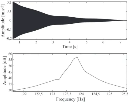
1 2 3 4 5 6 7 Time [s] 122 122,5 123 123,5 124 124,5 125 125,5 Frequency [Hz] Ampl itude [ dB ] Amplitude [m.s -2] 30 35 40 45 50 55 60 -0,2 0 0,2 0,1 -0,1
FIG. 4: Time waveform and spectrum of the first partial of the vibratory signal measured at point
A when string 31 is plucked. All strings are free to vibrate.
B. Method used for the extraction of modal parameters
1. Introduction: limit of the Fourier analysis
The Fourier spectrum of the accelerometer’s signal at point A is shown in Figure 3. When string 31 is plucked, several coupled modes of the system respond to produce the harp sound. This spectrum is composed of partials which are quasi harmonic. Using an appropriate selective filter, a zoom on this spectrum in the vicinity of the first partial and its corresponding time waveform are presented in Figure 4. This figure clearly shows that several sinusoidal components are present in the vibratory signal. Indeed, since free oscillations of the system occur, the response of the instrument to the plucking action measured by the
accelerometer, corresponds to the superposition of several modes whose frequencies are very close one to another. In the zoomed area of the spectrum, peaks of every component cannot be clearly separated whereas in the time waveform several sinusoidal components with different damping factors and frequencies appear. This shows the limit of the Fourier analysis. The presence of several vibration modes having close frequencies is a common characteristic for numerous free stringed instruments. Various methods, applied to musical instruments, such as techniques based on the Hilbert transform [4, 9] or High Resolution methods [4, 10, 11], allow the identification of spectral components.
For the identification of modes with close frequencies in the first partial, we choose to use a High Resolution method: the ESPRIT algorithm (Estimation of Signal Parameters via Rotational Invariance Techniques) [12]. A brief description of this technique and the specificity of its implementation in our context are given in paragraphs II B 2 to II B 4. An application to the harp’s signals is then presented in section II C.
2. The ESPRIT method
Subspace-based High Resolution methods such as the ESPRIT algorithm are of major interest for estimating mixtures of complex exponentials, because they overcome the spectral resolution limit of the Fourier transform and provide very accurate estimates of the signal parameters. These methods consist in splitting the observations into a set of desired and a
set of disturbing components, which can be viewed in terms of signal and noise subspaces. In this framework, the ESPRIT algorithm is based on a particular property of the signal subspace, referred to as the rotational invariance. This property permits to extract the model parameters from the eigenvalues of a so-called spectral matrix, which is obtained from the estimated signal subspace.
The noiseless Exponential Sinusoidal Model (ESM) defines the discrete signal x(t) as a sum of complex exponentials:
x(t) =
K
X
k=1
akeδktej(2πfk+ϕk), t ∈ [0, N − 1] (1)
where each frequency fk ∈ [−12,12] is associated to a real magnitude (ak > 0), a phase
(ϕk ∈ [−π, π]) and a damping or amplification factor (δk ∈ R). The whole number K is
the number of complex exponentials, also called model order, and N is the number of the
signal’s samples. By defining the complex amplitudes αk = akejϕk and the complex poles
zk = eδk+j2πfk, which are supposed to be distinct, the signal model x(t) can be re-written in
the following form:
x(t) =
K
X
k=1
αkzkt. (2)
to the K-dimensional signal subspace spanned by the Vandermonde matrix Vn = 1 1 · · · 1 z1 z2 · · · zK ... ... ... z1n−1 z2n−1 · · · zKn−1 .
It can be noted that this Vandermonde matrix satisfies the following rotational invariance
property: V↑ = V↓D, where D = diag(z1. . . zK), V↓ is the matrix extracted from V by
deleting the last row, and V↑ is the matrix extracted from V by deleting the first row.
In practice, the measured signal s(t) is corrupted by an additive noise: s(t) = x(t) + w(t), where w(t) is assumed to be white. Although matrix V is unknown, the signal subspace
can still be estimated as the principal eigensubspace of the correlation matrix ˆRss of the
measured signal, defined as follows:
ˆ Rss = 1 N − n + 1SS H , (3) where S = s(0) s(1) · · · s(N − n) s(1) s(2) · · · s(N − n − 1) .. . ... . .. ... s(n − 1) s(n) · · · s(N − 1) (4)
is the n × (N − n + 1) Hankel data matrix which involves N successive samples of the signal and the exponent H is the hermitian conjugate. Thus the n × K matrix W formed by the
K first principal eigenvectors of ˆRss is an orthonormal basis of the signal subspace.
Since the matrices W and V span the same subspace, there exists a K × K non-singular matrix G such that V = W G. It can then be noted that W satisfies an invariance
property similar to that of the Vandermonde matrix: W↑ = W↓Φ, where the K × K matrix
Φ = G D G−1, referred to as the spectral matrix, is similar to the diagonal matrix D. In
particular, the eigenvalues of Φ are the complex poles zk.
Finally, the ESPRIT algorithm consists of the following steps:
1. compute the signal subspace basis W by means of an eigenvalue decomposition,
2. compute the spectral matrix Φ by means of the least squares method:
Φ= W+↓W↑, (5)
where the symbol + denotes the Moore-Penrose pseudo-inverse,
3. estimate the complex poles zk as the eigenvalues Φ.
It is proved that the best performance in terms of statistical efficiency is obtained for a proper dimensioning of the data matrix S: n = N/3 or n = 2N/3 [11].
In a second stage, the complex amplitudes αk, grouped in a K × 1 vector denoted α, are
obtained thanks to the least squares method:
In equation (6), s denotes the vector containing N successive samples of the signal and
VN is the N × K Vandermonde matrix defined by the poles estimated by the ESPRIT
method. Parameters ak and ϕk are directly deduced as the modulus and phase of the
complex amplitudes αk.
3. Estimation of the number of components
The main difficulty of the method consists in evaluating the number K of components present in the signal. The technique commonly used is the over-estimation of this number and the discrimination of spurious results by means of an indicator such as the components energy or the error between the measured signal and the model. Other more effective methods exist for estimating the model order K such as the ESTimation Error (ESTER) method [11, 13] also used in the study. It consists in the computation of an inverse error function, J : p 7→ 1 k E(p) k2 2 (7) where E(p) = W↑(p) − W↓(p)Φ(p), (8)
for all possible orders 0 < p < n − 1. For determining the value of K, we choose the greatest value of p for which the function J(p) reaches a maximum which is greater than a threshold chosen arbitrarily above the noise level contained in the signal.
4. ESPRIT method implementation
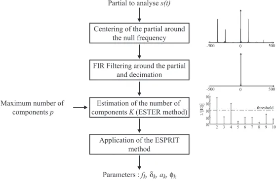
In order to minimize the computational time and increase the results accuracy [11], the ESPRIT method implementation is carried out according to the following procedure: after centering the studied partial around the null frequency, a finite impulse response (FIR) filter selects the frequency range containing the partial to analyse. The filter is chosen with a linear phase to keep the signal waveform. The filter is known to have a finite transitory response which corresponds to the length of its impulse response. The first filtered signal points belonging to this transitory phase are thus removed from the processing afterwards [4]. The filtered and centered signal is highly decimated to limit the computational time of the ESPRIT method. After the estimation of the model order by the ESTER method, as previously explained in section II B 3, the ESPRIT algorithm is then applied. The final validation of the model order is performed using a comparison between the measured and synthesized signals. An illustration of the method implementation is shown in Figure 5.
Note that in the Exponential Sinusoidal Model, the signal is assumed to be complex. For a musical sound, the signal is real and can be written as follows:
x(t) =
K
X
k=1
Akeδktcos(2πfkt + ϕk) (9)
which can be re-written with exponential terms:
x(t) = K X k=1 Ak 2 e δkt ej(2πfkt+ϕk) + K X k=1 Ak 2 e δkt e−j(2πfkt+ϕk) (10)
Maximum number of components p
Partial to analyse s(t)
Parameters : fk, δk, ak, φk Centering of the partial around
the null frequency
FIR Filtering around the partial and decimation
Application of the ESPRIT method
Estimation of the number of components K (ESTER method)
2 3 4 5 6 7 8 9 10 103 104 105 106 107 1/||E|| 2 2 0 -500 500 0 -500 500 threshold
FIG. 5: Summary of the implementation of the ESPRIT method on the studied partial.
Because of the filtering in the spectrum around the studied partial, the studied signal corre-sponds to the first part (with positive frequency) of the equation (10). In order to find the
real amplitude of the measured signal, the amplitude Ak obtained by the ESPRIT method
has to be multiplied by two.
C. Results
The implemented ESPRIT method, as previously explained, is applied to the signals measured on the concert harp in its final part, between 4s and 8s. The different experimental conditions are described in Table I and the attention is focused on the first partial of string 31. The estimated components found for this partial are gathered in Table II. The model
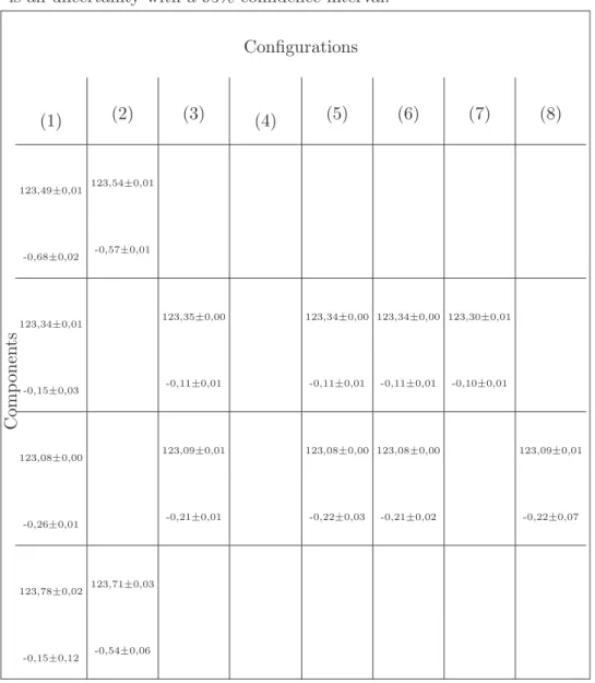
TABLE II: Frequencies and damping factors of identified components in the first partial of the
accelerometer signals in the eight experimental configurations defined in Table I. The reported
uncertainty is an uncertainty with a 95% confidence interval. Configurations C om p on en ts (1) (2) (3) (4) (5) (6) (7) (8) 123,49±0,01 123,54±0,01 -0,68±0,02 -0,57±0,01 123,34±0,01 123,35±0,00 123,34±0,00 123,34±0,00 123,30±0,01 -0,15±0,03 -0,11±0,01 -0,11±0,01 -0,11±0,01 -0,10±0,01 123,08±0,00 123,09±0,01 123,08±0,00 123,08±0,00 123,09±0,01 -0,26±0,01 -0,21±0,01 -0,22±0,03 -0,21±0,02 -0,22±0,07 123,78±0,02 123,71±0,03 -0,15±0,12 -0,54±0,06
order stretches from 0, for configuration (4), to 4, for configuration (1). Note that for each configuration, coefficients are computed from 5 measurements for estimating a repeatability uncertainty. In Table II, the components are classified in such a way that their amplitude are in descending order from top to bottom. Moreover, they are aligned in order to facilitate
the reading of the missing components.
From a general point of view, the repeatability uncertainties calculated for different pa-rameters are extremely small, lower than 1% for the frequencies and around 10% for the damping factors. Nevertheless, for some components the uncertainty can be important as for the last component of the (1) configuration. This can happen for components not very present, with a weak energy, and a weak signal-to-noise ratio.
When the instrument is not modified ((1) and (3) to (8) configurations) the components’ parameters slightly vary, less than 0,5% for the frequencies and, in a maximum of 30% of variation for the damping factors. This result shows that the stopped string does not modify the vibratory behavior of the instrument. Nevertheless, when paper is added to damp all strings except string 31, in configuration (2), the components’ damping factors are modified and a slight shift in frequency is caused. The instrument is slightly modified by the added paper but not enough to allow the identification of the components’ nature.
Thanks to the developed experimental protocol and the identification method, the com-ponents present in the first partial are obtained. The results show that the estimated parameters are stable following the eight experiences. These results are compared in the following section to the modal basis of a simplified harp.
III. THEORETICAL STUDY OF THE HARP’S SYMPATHETIC MODES
A. Description of the model
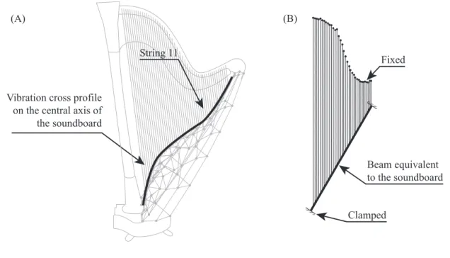
Vibrations of the studied concert harp have been investigated in a previous paper [1] thanks to an experimental modal analysis. In low frequencies, six consecutive modes have been identified from 24 Hz to 181 Hz. The investigation of the mode shapes show two particular characteristics: mode shapes are symmetric according to the strings plane and for all modes, the bending motion of the soundboard is similar to the first mode shape of a clamped-clamped beam. Thus, although the soundboard is a complex assembly, constituted of a sandwich of several layers of different wood glued together reinforced by a central aluminum bar and by two lateral stiffeners in wood, the soundboard can be described by using an equivalent beam clamped at both ends. The typical first bending mode at 152.2 Hz is shown in Figure 6-A and its corresponding mode shape can schematically be described as an important deflection in the lower two thirds of the soundboard between the two clamped points, one at the pillar level and the other one at the 11-string level. Indeed, on the treble strings, the soundboard is rigidified by the proximity of the edge linked to the soundbox, explaining the absence of movement in low frequencies. Thus, the beam length clamped at both ends is limited to the distance included between the harp’s pillar and the 11-string. According to this experimental result, the vibratory model is composed of a 1m-long beam
Vibration cross profile on the central axis of the soundboard Beam equivalent to the soundboard Clamped Fixed (A) (B) String 11
FIG. 6: (A) Modal shape associated to the fourth mode and description of the vibratory profile in
the central axis of the soundboard. (B) Model of the concert harp: beam-35 strings assembly.
on which 35 strings are attached as shown in Figure 6-B.
The mechanical properties of the equivalent beam and of each string have to be deter-mined: for the strings, most parameters are directly measured on the harp [14] except for the Young’s modulus and the density which are supposed to equal the data given in [15] and [16]. Values of the tension are computed from the fundamental frequency of the tones, by considering strings fixed at both ends. For the equivalent beam, the determination of its pa-rameters is more complicated since the geometrical papa-rameters are directly measured on an
isolated soundboard, allowing the evaluation of a mean density (ρ = 553 Kg/m3). The area
along the axis. Average values of these two parameters are thus retained to characterize
the equivalent beam (Aeq = 38.3 cm2 and Jeq = 38.9 cm4). Finally, the Young’s modulus
E of the equivalent beam is determined so that the first bending mode of the beam in the beam-35 strings assembly equals 150 Hz, the eigenfrequency of the fourth mode shown in Figure 6-A (E = 5.9 GPa).
The vibratory model of the harp can thus be considered as an assembly of an equivalent beam connected to 35 strings as described in Figure 6-B. This vibratory model is afterwards named the simplified harp.
B. Harp’s sympathetic modes
The modal basis of the simplified harp is computed using the transfer matrix method, which is appropriated for modeling assemblies of one-dimensional sub-structures. This com-putation is based on a wave guide model for each sub-structure of the beam-strings assembly. A brief summary of the different steps of the method is proposed in appendix and details are developed in [8]. Eigenfrequencies are obtained for singularities of a characteristic
ma-trix labeled RR (see equation (15) page 31). Each drop of the logarithm of matrix RR’s
determinant, defined in equation (16), corresponds to an eigenfrequency.
Modes of the system are computed in the frequency range [0-500 Hz] by step of 0.01 Hz
Mode 26 Mode 27 Mode 28 Mode 33 110 120 130 140 150 160 298 296 294 292 290 288 286 284 282 Frequency [Hz] L og(det(R R )
FIG. 7: Logarithm of the determinant of the characteristic matrix RR as function of frequency.
Each drop corresponds to an eigenfrequency of the beam-strings assembly.
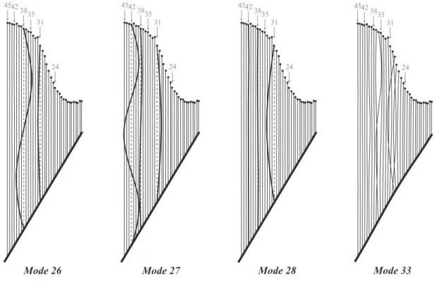
4542 3835 31 24 4542 3835 31 24 Mode 26 Mode 27 454238 35 31 24 Mode 28 Mode 33 4542 3835 31 24
FIG. 8: Mode shapes associated to modes 26, 27, 28 and 33. The number indicated below the
[110-160 Hz], showing that modes have very close eigenfrequencies. Among the 151 modes found in the range [0-500 Hz], examples of four modal shapes are presented in Figure 8. These shapes clearly show that for each mode each substructure does not interact in the same manner. To classify modes of the assembly, we use a criterion called Kinetic Energy Ratio (KER) defined by
KERj(k) = Z lk 0 ρkΨTj(x)Ψj(x) dx X r Z lr 0 ρrΨTj(x)Ψj(x) dx . (11)
In this equation ρ is the mass per unit length of the sub-structure, Ψj is the mode shape of
mode j and x is the generic space variable defined in the Appendix. The KER corresponds
to the ratio of kinetic energy of one sub-structure k (of length lk) divided by the total
kinetic energy of the structure. Its value is a percentage and allows us to identify the relative importance of each sub-structure displacement field. In the study, this percentage is rounded to the nearest whole number. Thus, for a given mode, a null value of the KER of a sub-structure indicates that this sub-structure is inactive. Values of KER on each sub-structure are used to classify modes into four groups [8]: beam modes, string modes, string-string modes, beam-string modes.
In Table III, the eigenfrequencies and KER of each sub-structure of modes 26, 27, 28 and 33 are reported. For these four modes, the KER is significant only for four sub-structures:
the beam and strings 31, 38 and 42. String 31 (Cb3 note of fundamental frequency 123.5 Hz)
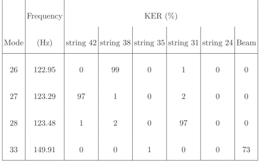
TABLE III: Eigenfrequencies and Kinetic Energy Ratio for each sub-structure (strings 42, 38, 35,
31, 24 and the beam). KER expressed in % and rounded to the nearest whole number.
Frequency KER (%)
Mode (Hz) string 42 string 38 string 35 string 31 string 24 Beam
26 122.95 0 99 0 1 0 0
27 123.29 97 1 0 2 0 0
28 123.48 1 2 0 97 0 0
33 149.91 0 0 1 0 0 73
which is the upper fifth of string 42 (Fb1 at fundamental frequency 41.2 Hz). The beam’s
KER nearly equals zero for modes 26 to 28, showing that mode shapes are dominated by the string’s motion since the KER is distributed according to two or three strings, allowing the definition of these modes as string-string modes or sympathetic modes [8]. Actually, according to the modal superposition principle, if string 31 is plucked, modes 26 to 28 are set into vibration and so are strings 38 and 42, generating the phenomenon of sympathetic vibrations. Note that for these three sympathetic modes, modifications of the character-istics of the equivalent beam only slightly modify the KER distribution, not altering our conclusions. Nevertheless, it appears that for other vibratory modes the KER distribution can be affected.
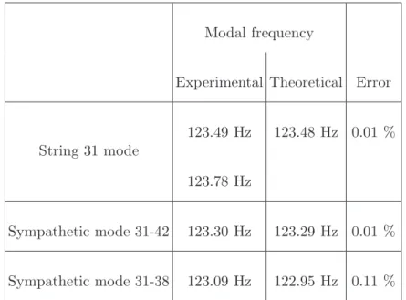
TABLE IV: Comparison between experimental and theoretical results obtained from the vibratory
model of the concert harp.
Modal frequency
Experimental Theoretical Error
String 31 mode 123.49 Hz 123.78 Hz 123.48 Hz 0.01 % Sympathetic mode 31-42 123.30 Hz 123.29 Hz 0.01 % Sympathetic mode 31-38 123.09 Hz 122.95 Hz 0.11 % IV. DISCUSSION
When string 31 of the concert harp is free to oscillate (configuration (1) in Table I), two sinusoidal components are identified in the first partial. When this string is stopped (config-urations (2), (3) and (4)), these two components disappear. In playing configuration, these two sinusoids have close frequencies, separated by only 0.2 Hz, and have very different damp-ing factors and amplitudes. This result thus points out that the strdamp-ing vibrates followdamp-ing its two polarizations. These two polarizations are excited by the harp player in a different way depending on the string plucking, involving different initial amplitudes (showed by the difference of energy of each component). Moreover, as for the piano, one of the polarizations seems to be favored for transmitting its energy to the soundboard, implying a rapidly
de-caying component at the plucking moment [2]. This result shows that for a good modeling of the strings’ modal behavior, the two polarizations of string vibrations have to be taken into account. In the simplified harp, only one polarization is considered, which constitutes a limitation.
When the string is stopped during the oscillations, modes present in the instrument response are selected. In configurations (3), (5) and (6), the same components are present, showing that modes implying strings 24 and 35 do not participate in the first partial of the instrument response. By stopping strings 31 and 38, one vibrating component disappears and by stopping strings 31 and 42, another one is absent from the instrument’s response. With configurations (7) and (8), we can deduce that strings 38 and 42 participate in the sound radiated by the instrument.
When the harpist plucks string 31, four modes are set into vibrations at the same time: two modes involving string 31 (one mode per polarization), one mode involving strings 31-38 and one mode involving strings 31-42. These last two modes are thus sympathetic modes. The stopping of string 31 does not necessary lead to the weakening of these modes, proving that the kinetic energy present in strings 42 and 38 is definitely more important than in string 31. Moreover, these results show that the sympathetic modes coming from each polarization of string 31 are not visible in the response. This fact can be explained by the weak energies of these modal components, not allowing them to emerge from the noise.
These experimental results can be compared to those obtained from the theory. Experi-mentally, we found two modes which mostly involve string 31 at 123.59 Hz and at 123.78 Hz. With the vibratory model, the string mode associated to string 31 is found at 123.48 Hz. Note that the model takes only one string polarization into account. The agreement between model and measurement is, as expected, very good since the tension value of each string of the simplified harp has been fixed in such a way that the eigenfrequencies of uncoupled strings correspond to those of the real instrument.
For sympathetic modes 31-42 and 31-38, their eigenfrequencies are measured at 123.28 Hz and at 123.08 Hz. It should be noticed that the theoretical eigenfrequencies of these modes are found at 123.29 Hz and at 122.95 Hz, coinciding almost perfectly with experimental results. Apart from the fact that the vibratory model of the concert harp does not take the two polarizations of the string into account, results obtained from the model are in very good agreement with those obtained during experiments, thus validating the vibratory model of the beam-35 string assembly of the concert harp.
V. CONCLUSION
The numerous strings of the concert harp induce sympathetic vibrations, which are re-sponsible for the feeling of halo of sound. This characteristic is important and constitutes a signature of the instrument. In this paper, experimental and theoretical investigations have
been carried out to understand this phenomenon. The following conclusions can be drawn. (a) It has been shown that sympathetic modes, responsible of the sympathetic vibrations, are present in the instrument’s response. These sympathetic modes are due to the coupling between different strings via the soundboard. With a waveguide model of the harp, their eigenfrequencies and mode shapes can be accurately determined. This model describes bend-ing and longitudinal motions in the strbend-ings, connected to an equivalent beam representbend-ing the soundboard and allows the modal basis of the strings-beam assembly to be computed.
(b) In the time domain, sympathetic vibrations generate multiple components in the string’s partials. Resolution of the Fourier analysis does not permit their identification. This identification is performed using the ESPRIT method, which is a High Resolution method. The determination of the number of elementary spectral components, which is the main difficulty in the implementation of High Resolution methods is successfully performed using the ESTER method.
(c) Several components are identified in the first partial of string 31: two of them corre-spond to two strings modes having different polarizations. Other components correcorre-spond to sympathetic modes. In the analysed example, two sympathetic modes are involved. Their number and their eigenfrequencies are very well captured by the proposed model.
Although the model of the instrument suits the identification of sympathetic modes, it can be extended in order to take into account two polarizations per strings. Moreover,
from an experimental point of view, the analysis of partials of higher order, where other phenomena such as octave vibrations can be present, could also be performed.
Appendix: determination of the beam-strings assembly modes
In this appendix, we summarize the method for computing normal modes of the beam-strings assembly, illustrated in Figure 9. The detailed method is published in [8].
O1 C1 Ci CN Oi ON yb xb ysi xsi
FIG. 9: Diagram of a clamped-clamped beam connected to several fixed strings. It includes local
coordinate systems.
In harmonic regime, the vibratory state of each sub-structure (string and beam) of the assembly is described at any point of its neutral line by a state vector X (x) whose
compo-nents are kinematic and force variables. Variable x is the spatial coordinate describing the current point on the sub-structure. For the string, the state vector is the following vector:
Xs(x) = us(x) ws(x) Ns(x) Qs(x)
!T
, (12)
where us, ws are longitudinal and transversal displacements and Ns, Qs are the longitudinal
and transversal forces. In the beam, the state vector is written as follows:
Xb(x) = ub(x) wb(x) θb(x) Nb(x) Qb(x) Mb(x)
!T
, (13)
where ub, wb and θb are respectively the longitudinal and transversal displacements and the
slope of the beam cross section, and where Nb, Qb and Mb are respectively the longitudinal
and transversal forces and the bending moment. With the transfer matrix method, it can be shown that the vibratory state of each sub-structure at any point x can be expressed in
function of the vibratory state at another point x0 with the following expression:
X (x) = T(x, x0)X (x0), (14)
where T(x, x0) is the transfer matrix of the sub-structure (beam or string) between the
state vector at point x0 and the state vector at point x. By using coupling equations at
beam-string connection [8], it can be shown that the force components of state vectors on
boundary Xf verify the following equation:
where RRis defined as a characteristic matrix of the assembly. In the case of free vibrations,
vector Xf is not equal to zero and the matrix R
R is not invertible, implying:
det (RR(ω)) = 0. (16)
The angular eigenfrequencies ωi of the system are obtained as the solutions of
equa-tion (16). For each ωi, relation (15) provides the components of Xf from which we can
calculate all state vector components at any point on the assembly.
Acknowledgement
The authors acknowledge the instrument maker CAMAC Harps for the lending of the concert harp.
[1] J-L. Le Carrou, F. Gautier & E. Foltˆete: Experimental study of A0 and T1 modes of the
concert harp. J. Acoust. Soc. Am. 121 (2007) 559-567.
[2] G. Weinreich: Coupled piano strings. J. Acoust. Soc. Am. 162(6) (1977) 1474-1484.
[3] X. Boutillon: Measurement of the three-dimensional admittance at a violin bridge. In
pro-ceedings of the 13th International Congress of Acoustics, Belgrade, Serbia (1989).
[4] B. David: Caract´erisations acoustiques de structures vibrantes par mise en atmosph`ere
pro-pres. Applications en acoustique musicale (Acoustical characterization of vibrating structures
in near vacuum. Estimation methods for eigenfrequencies and damping factors. Applications
in musical acoustics). PhD Thesis, Universit´e Paris 6, Paris, France (1999).
[5] B. Capleton: False beats in coupled piano string unisons. J. Acoust. Soc. Am. 115 (2004)
885-892.
[6] J. Dickey: The structural dynamics of the American five-string banjo. J. Acoust. Soc. Am.
114(5) (2003) 2958-2966.
[7] C. Erkut, M. Karjalainen, P. Huang & V. V¨alim¨aki: Acoustical analysis and model-based
sound synthesis of the kantele. J. Acoust. Soc. Am. 112(4) (2002) 1681-1691.
[8] J-L. Le Carrou, F. Gautier, N. Dauchez & J. Gilbert: Modelling of sympathetic string
vibra-tions. Acta Acustica United with Acustica 91(2) (2005) 277-288.
[9] L. Rossi and G. Girolami: Instantaneous frequency and short term Fourier transforms:
appli-cation to piano sounds. J. Acoust. Soc. Am. 110(5) (2001) 2412-2420.
[10] J. Laroche: The use of the matrix pencil method for the spectrum analysis of musical signals.
J. Acoust. Soc. Am. 94(4) (1993) 1958-1965.
[11] R. Badeau: M´ethodes `a haute r´esolution pour l’estimation et le suivi de sinusoides modul´ees.
Application aux signaux de musique. (High resolution methods for estimating and tracking
modulated sinusoids. Application to music signals). PhD Thesis, T´el´ecom Paris, Paris, France
[12] R. Roy, A. Paulraj et T. Lailath: ESPRIT - A subspace rotation approach to estimation of
parameters of cisoids in noise. IEEE Transactions on Acoustics, Speech and Signal Processing
34(4) (1986) 1340-1344.
[13] R. Badeau, B. David and G. Richard: A new perturbation analysis for signal enumeration
in rotational invariance techniques. IEEE Transactions on Signal Processing 54(2) (2006)
450-458.
[14] J-L. Le Carrou: Vibro-acoustique de la harpe de concert (vibro-acoustics of the concert harp).
PhD Thesis. Universit´e du Maine, Le Mans, France (2006).
[15] A.J. Bell and I.M. Firth: The physical properties of gut musical instrument strings. Acustica
60(1) (1986) 87-89.
[16] A.J. Bell: An acoustical investigation of the Concert Harp. PhD dissertation, University of St