HAL Id: hal-01699827
https://hal.inria.fr/hal-01699827
Submitted on 2 Feb 2018
HAL is a multi-disciplinary open access
archive for the deposit and dissemination of
sci-entific research documents, whether they are
pub-lished or not. The documents may come from
teaching and research institutions in France or
abroad, or from public or private research centers.
L’archive ouverte pluridisciplinaire HAL, est
destinée au dépôt et à la diffusion de documents
scientifiques de niveau recherche, publiés ou non,
émanant des établissements d’enseignement et de
recherche français ou étrangers, des laboratoires
publics ou privés.
A Use-Case Study on Multi-view Hypothesis Fusion for
3D Object Classification
Panagiotis Papadakis
To cite this version:
Panagiotis Papadakis. A Use-Case Study on Multi-view Hypothesis Fusion for 3D Object
Classifi-cation. ICCVW 2017 - IEEE International Conference on Computer Vision Workshop, Oct 2017,
Venice, France. �10.1109/ICCVW.2017.288�. �hal-01699827�
A Use-Case Study on Multi-View Hypothesis Fusion
for 3D Object Classification
Panagiotis Papadakis
IMT Atlantique Bretagne-Pays de la Loire, LabSTICC UMR 6285, team IHSEV
Technopˆole Brest-Iroise, France
Abstract
Object classification is a core element of various robot services ranging from environment mapping and object ma-nipulation to human activity understanding. Due to lim-its in the robot configuration space or occlusions, a deeper understanding is needed on the potential of partial, multi-view based recognition. Towards this goal, we benchmark a number of schemes for hypothesis fusion under different en-vironment assumptions and observation capacities, using a large-scale ground truth dataset and a baseline view-based recognition methodology. The obtained results highlight important aspects that should be taken into account when designing multi-view based recognition pipelines and con-verge to a hybrid scheme of enhanced performance as well as utility.
1. Introduction
View-based methods for object classification have been shown in latest extensive experiments [4], [16] to out-match 3D-based shape description methodologies of com-plete shapes. Such results are particularly encouraging for robotic applications since observing objects from multiple viewpoints is often infeasible either due to robot kinematic constraints or due to the presence of obstacles. On the other hand, it is generally true that not all viewpoints are equally informative in discriminating the class of an object. This is because the discriminative features of an observation taken from a particular viewpoint depend on the intra-class as well as inter-class variability as well the nature of the underlying features that are extracted (cf. Fig 3., [19]). As a conse-quence, there is an unavoidable bias/utility towards certain viewpoints when classifying objects depending on the shape of the object and its semantic class (cf. Fig. 2, [8] and Fig. 3, [11]). Therefore, while an integral inspection of an object may not be necessary for correct classification, we can ex-pect that in the worst case two or more observations will be
required in order to capture the most discriminative object parts.
Most earlier works addressing multi-view object classifi-cation are appliclassifi-cation oriented with predetermined assump-tions. The authors of [8] exploit the viewpoint bias of de-tectors only empirically by adopting the shape description method with the highest influence to viewpoint variability and mostly evident among positive and negative examples. To fuse the classification outputs obtained from the total set of observations they apply the naive Bayes criterion, also applied in their consecutive work [9].
In the work of Becerra et al. [2] a POMDP formulation for confirming the class of an object is proposed which in-tegrates information on robot location and the output of an object detector. A solution is found via stochastic dynamic programming for a fixed time horizon, but only after assum-ing a particular class for the object of interest before tryassum-ing to optimize the detection score while performing training and testing on the same object. This makes that approach unsuited when the objective is to confirm one among many possible classes and on different test and train objects.
Potthast et al. [12] also adopt a POMDP formulation for joint category and viewpoint classification of an object by further incorporating feature selection on interleaved steps of local and global optimization. Since their main goal is to extract the optimal category and viewpoint at the last obser-vation of an object with no concern on the consistency along the entire observation sequence, state transitions among cat-egories are not excluded which could lead to unreasonable results.
In [1] the authors propose a model for active object clas-sification and pose estimation that jointly considers sensor movement and decisional cost. They are also based on a POMDP formulation, yet its practical utility is limited be-cause successive observations are considered independent and state transitions among object categories are also al-lowed. Their experiments also appear to be limited by con-sidering only 1 object category at a time.
are estimated separately and by assuming observation inde-pendence for both problems. The class distribution is ob-tained by Bayesian updates while pose by the best align-ment among all observations and the best match given by the classifier, through Iterative Closest Point (ICP) registra-tion.
Overall, due to differences in the applications, assump-tions and detectors among earlier works it is not straightfor-ward to derive conclusions on the conditions under which multi-view classification is beneficial compared to single-view object classification.
In this work, we examine the performance of multi-view hypothesis fusion for 3D object classification both under observation dependence or independence and in consider-ation of the robot observconsider-ational capacities. Under observa-tion dependency, we detail how multiple classes can be hy-pothesized by firstly evaluating the viewpoint sequence es-timation problem for every hypothesized class and secondly by assigning the class with the highest overall probability. After comparison against alternative fusion schemes under observation independence, the experiments highlight that it proves consistently beneficial with the increase of distinct observations, in contrast to observation dependence which proves superior only early in the observation sequence.
The remaining of the article is organized as follows. In Section 2 we formulate the problem under consideration, in Section 3 we describe different hypothesis fusion schemes along with the conditions and assumptions that are applica-ble for each case and in Section 4 we evaluate crucial as-pects of multi-view based object classification on a public dataset.
2. Problem Description
We treat the problem of optimal classification of static or dynamic 3D objects from sequences of observations ac-quired from multiple viewpoints by a mobile sensor. A ground truth of labelled object templates observed from var-ious viewpoints is assumed available where each annotated training sample is a tuple composed of the semantic class of the object, the observed viewpoint and the correspond-ing feature vector. Considercorrespond-ing the observation viewpoint as part of the ground truth implies that objects that belong to the same semantic class of the ground truth must share a fixed canonical pose, namely, they are aligned to each other as in the case of ModelNet [20] or CAPOD datasets [10].
When exploring a new environment, i.e. during testing, both the semantic class as well as the pose of an object are unknown and thus the challenge resides in devising them from the collected observations. In the context of a robotic application, we are generally more interested in hypothe-sizing the semantic class and secondarily the pose since the latter can be ambiguous or even absent due to shape symme-try across object views. Object classification will therefore
be used as the final performance measure criterion. To address the outlined problem, we may rely on: (i) a capacity to hypothesize the semantic class and the observed viewpoint of an object based on a single frame/observation and (ii) an approximate sensor localization capacity. The first capacity allows only for joint consideration of differ-ent observations under the assumption that they are inde-pendent while the second capacity allows to enforce depen-dency between successive observations. Upon presenting these capacities in sections 2.1, 2.2 we then detail the fusion schemes that can be considered depending on assumptions in Section 3.
2.1. Single Observation Model
A feature vector classification method is employed (see Sec. 4) which classifies a given feature vector x describing an object ox to one of |I| classes ωi ∈ I, i ∈ {1, 2, ...|I|}
based on the corresponding probability P (ωi|x). A feature
vector corresponds to the global shape descriptor extracted by observing an unknown object from an unknown view-point. If we assert that an object ox belongs to a specific
class ωi, we write ox= ωi.
For the evaluation of the posterior probability P (ωi|x),
a nearest neighbor classification scheme is adopted which sets the probability as inversely proportional to the match-ing distance between x and the nearest neighbor that be-longs to ωi, namely: P (ωi|x) ∝ dist 1 N N(x,ωi) (1) distN N(x, ωi) = min y∈Y|oy=ωi dist(x, y) (2)
where Y is the total set of feature vectors of the ground truth database that are compared against x and dist(., .) is the distance function for a pair of feature vectors.
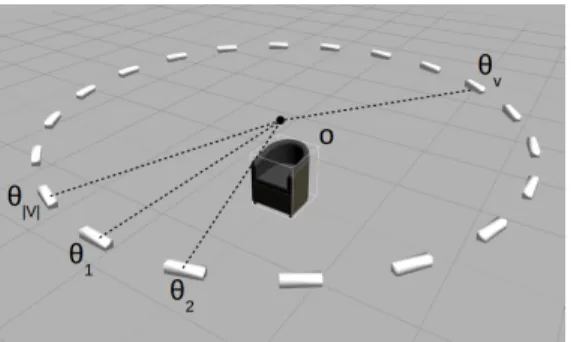
The total number of possible classes is therefore |I| = |V | · |S| where |V | is the cardinality of the set of view-points V from which each object is observed and |S| the cardinality of the set of object semantic classes S. It fol-lows that each ωi is associated with a particular object
viewpoint θv = (v − 1)2π/|V |, v ∈ {1, 2, ...|V |} of a
particular semantic class cs, s ∈ {1, 2, ...|S|}, which can
be equivalently denoted as ωvsthrough the linear mapping
i = v + (s − 1)|V |. We will hereafter employ the two nota-tions ωi and ωvs interchangeably for convenience
depend-ing on the context. Fig. 1 depicts the underlydepend-ing notations with a representative object of semantic class armchair.
2.2. Sensor Localization and Transition Model
We consider a mobile robotic sensor with the capability of aproximate 2D localization around an object of interest, e.g. following the approach described in [6]. The location of the sensor is used for measuring its displacement across
Figure 1. Example object and observation configuration
succesive observations and in turn, obtain the expected tran-sition/shift in the observed object pose. Considering a se-ries of observations where k ∈ {2, 3..., N } denotes the ob-servation step, we can readily obtain the transition prob-ability p(ωv(k)s(k)|ωv(k−1)s(k−1)), where ωv(k)s(k) is one
of the possible classes that can be appointed to an object at the kthobservation step, i.e. v(k) ∈ {1, 2, ...|V |} and s(k) ∈ {1, 2, ...|S|}.
Recalling subsection 2.1, each class ωi can be
equiva-lently referred as ωvswhere v and s correspond to a
view-point and a semantic object class respectively. Evidently, when observing a particular object there can only be transi-tions between viewpoints and not among semantic classes. Therefore, we simplify the transition probability as:
p(ωv(k)s|ωv(k−1)s) = N (∆α; µ∆θk, σ) (3)
where µ∆θk = θv(k)− θv(k−1)is the angle between
view-points v(k) and v(k − 1), σ corresponds to the standard deviation that quantifies the uncertainty of the sensor local-ization and ∆α the angular displacement of the sensor with respect to the object between observations k − 1 and k.
3. Fusion schemes
3.1. Hypothesis Fusion based on Observation
De-pendency
We first investigate the possibility of fusing the total number of obtained hypotheses by assuming dependency among observations, which implies using both capacities described in Sections 2.1, 2.2. Given a sequence of object observations xk, the optimal class is obtained as:
ω∗i(N )= argmax
ωi(N )
Dmax(ωi(N )) (4)
where Dmax(ωi(N )) is the maximum decision score that
can be deduced if class ωi(N ) ∈ I is matched to the
un-derlying object.
The above problem can be formulated as a hidden markov model (HMM) where ωi(k) are the possible,
hid-den states along the observation sequence and xk are the
corresponding observations. In this context, the aggregated decision cost at time step k is given by:
D(ωi(k)) = k
X
r=1
d(ωi(r), ωi(r−1)) (5)
where d(ωi(r), ωi(r−1)) is the cost that is associated to a
transition between succesive states ωi(r) and ωi(r−1).
Al-though the term cost may seem counterintuitive since we seek to maximize eq. (4), it is adopted here for the sake of correspondence to the literature (cf. [17], Ch. 9) which further holds true for the chosen notations.
Recalling that when observing a particular object the only possible state transitions concern transitions between viewpoints and not among semantic classes, it follows that eq. (5) can be expressed as:
D(ωi(k)) = D(ωv(k)s) = k
X
r=1
d(ωv(r)s, ωv(r−1)s) (6)
where the decisional transition cost d(., .) is defined as:
d(ωv(k)s, ωv(k−1)s) = ln(p(ωv(k)s|ωv(k−1)s) · p(xk|ωv(k)s)) (7)
where p(ωv(k)s|ωv(k−1)s) is obtained by eq. (3) and the
likelihood function p(x|ωi) introduced in eq. (7) is
ob-tained by applying Bayes rule and assuming equal a priori class probabilities. In other words, we do not assume that certain object classes are more likely to appear than others, although such treatment could be employed when the sur-rounding spatial context can be accounted for (cf. [5] and [7]). In this way, we obtain that p(x|ωi) ∝ P (ωi|x)/p(x)
which makes the calculation of p(x) redundant in the evalu-ation of the cost in eq. (7). Eventually, the maximizevalu-ation of the aggregated cost D is efficiently calculated via dynamic programming by virtue of Bellman’s principle and by em-ploying the Viterbi algorithm [18].
3.2. Hypothesis Fusion based on Observation
Inde-pendence
Observation independence is assumed in the case of no sensor localization capacity or whenever we cannot assume that objects remain strictly static along the entire set of ob-servations, therefore all state transitions are equiprobable. Under such conditions, we examine a number of possible hypothesis fusion schemes presented as follows.
3.2.1 Equiprobable Transitions
The first scheme can be considered as a subcase of the pre-vious by setting the transition probability to be uniformely distributed, i.e. p(ωv(k)s|ωv(k−1)s) = 1/|V |. This implies
that the transitional decision cost of eq. (7) depends only on the observation likelihood while the optimal class ωi(N )∗ is obtained in the same manner using Viterbi algorithm.
3.2.2 Maximum Similarity
In this scheme, we hypothesize as class of the object the one corresponding to the viewpoint observation with the maxi-mum probability, namely:
ω∗i(N )= argmax
ωi(k)
P (ωi(k)|x)) (8)
where P (ωi(k)) is calculated using eq. (1).
3.2.3 Maximum Certainty
We hypothesize as class of the object the classification re-sult of the viewpoint observation with the maximum classi-fication certainty, namely:
ω∗i(N )= argmin ω∗ i(k) Hi(k) (9) ω∗i(k)= argmax i P (ωi(k)|x) (10)
Hi(k)= −PiP (ωi(k)|x) log P (ωi(k)|x) (11)
and certainty is quantified via Shannon’s information en-tropy.
4. Results
We performed a comparative evaluation of the afore-mentioned approaches within the Princeton ModelNet10 [20] dataset which contains 4899 objects distributed into 10 common indoor classes, in order, bathtub, bed, chair, desk, dresser, monitor, night stand, sofa, table and toilet. These categories correspond to the top 10 most common indoor object categories according to [21]. Example 3D objects for each category are shown in Fig. 2.
Figure 2. Example 3D objects from ModelNet10 dataset categories
This dataset is particularly suited in the context of a mo-bile robotic sensor since the pose of each synthetic object coincides with its expected upright orientation in the real world, which in turn allows the adoption of a fixed sensing configuration. For our experiments, we set M = 20 cam-era viewpoints uniformly distributed around each object at a sensor pose that is orientated versus the centroid of the coordinate system at a fixed pitch angle. This testing con-figuration is equivalent to related works on multi-view ob-ject classification such as [16], [12] or [4] wherein a roving sensor observes a query object from different viewpoints and estimates its class and possibly its pose. Nevertheless,
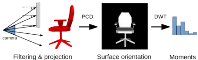
Figure 3. Baseline method for single observation model Table 1. Comparative classification performance of baseline single view observation model against state-of-the-art methods
Precision % Recall % Baseline 71.4 70.9 ESF [19] 73.6 72.8 VFH [13] 69.9 69.1 ROPS [3] 58.3 57.7
the scope of our evaluation is different in that we do not seek to compare the performance among different single-view based object recognition methods but among decision fusion schemes based on a common, baseline single-view method.
The baseline approach that we adopt here for the sin-gle observation model assumed in Sec. 2.1 is composed of the following steps. First, a bilateral filter is applied on a depth buffer image acquired by simulating a perspective projection of the object using as intrinsic camera parameters those corresponding to a Kinect V1 sensor. The smoothed organized point cloud (PCD) is then used to compute the surface orientation at each sensed point, producing a sur-face orientation image. That image is finally encoded by a multi-scale 2D discrete wavelet transform (DWT) whose coefficients are used to extract a set of central moments (mean, standard deviation and skewness) for each distinct wavelet sub-band and scale. To compare two feature vec-tors, the Canberra distance score is employed. This feature extraction procedure is summarized in Fig. 3. As a ref-erence for the general performance of our baseline single observation model, we further provide in Table 1 its com-parative performance to three other state-of-the-art single-view based object descriptors in terms of precision and re-call. The compared methods are: (i) Ensemble of Shape Functions (ESF) [19], (ii) Rotational Projection Statistics (RoPS) [3] and (iii) VFH (Viewpoint Feature Histograms) [13], whose implementations are available with PCL (Point-Cloud Library) [14]. These results suggest that the adopted baseline observation model is representative of the state-of-the-art performance.
To evaluate performance among hypothesis fusion schemes, we calculate the precision and recall scores for each object class and perform leave-one-out experiments by simulating sensor observations from randomly chosen
viewpoints and k ∈ {2, 3, ..., 6}. We perform a total of 4 independent runs for each k and fusion scheme and finally obtain the average.
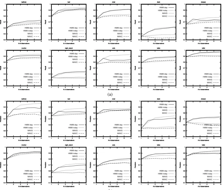
We abbreviate the compared hypothesis fusion schemes as follows: HMM-dep (Sec. 3.1), HMM-indep (Sec. 3.2.1), MAXS (Sec. 3.2.2) and MAXC (Sec. 3.2.3). In Fig. 4 we demonstrate the respective results for each class of the dataset, for both precision and recall scores. For the trivial case of 1 observation being considered, since there is no hypothesis fusion all schemes attain the same per-formance. When multiple observations are performed for (k = 2, 3, ...) the presented results are instructive in a num-ber of points.
First of all, we observe that the consideration of supple-mentary viewpoint observations contributes almost always in the increase of classification performance (with the ex-ception of the desk Recall and the dresser precision when using the MAXC criterion). The first 3 observations ap-pear to be in general those which contribute the most while performance seems to stabilize afterwards with very little additional benefit. Furthermore, it is clear that the average macroscopic performance for schemes MAXS and MAXC is clearly inferior compared to the other alternatives. This strongly suggests that single-view based object classifica-tion cannot alone surpass the performance of multi-view classification. If this is the case then this result may ap-pear contradictory to the results presented in [15] where view-based methods surpass entire 3D object discrimina-tion methods.
An explanation to this contradiction emerges via the comparison between the schemes dep and HMM-indep. Considering observation dependence via HMM-dep is consistently beneficial when k = 2 observations, while for more observations the performance seems to stabilize in an abrupt way and sometimes even decrease (see dresser Recall, sofa Recall, bed Precision, chair Precision, toilet Precision). Conversely, considering observation indepen-dence via HMM-indep, performance is always favoured by the consideration of supplementary observations and con-vergence is smoother and in turn, more stable. Furthermore, HMM-indep surpasses HMM-dep in the majority of classes both in terms of precision and recall while achieving very close performance to HMM-dep in the remaining cases.
The above observations leads us to the principal outcome of the experiments, namely, that multi-view object classifi-cation is strongly influenced on the underlying assumptions (i.e. viewpoint dependency) and occasionally by the object category. The fact that viewpoint independence appears to generally be more beneficial than considering dependency, means that there may be classes easier to be confused if they exhibit similar visual characteristics when observed from the same viewpoints. In such cases, observation indepen-dence allows an observation to be matched to an arbitrary
Table 2. Average macroscopic performance of hypothesis fusion schemes as a function of supplementary observations
Recall/Precision per number of observations Fusion schemes 2 3 4 5 6 HMM-dep 78.8/79.7 79.9/80.8 80.7/81.5 81.3/82.2 81.8/82.7 HMM-indep 77.8/78.7 81.4/82.9 82.1/83.6 82.6/84.2 83.1/84.6 MAXS 73.4/73.8 75/75.6 75.4/76.1 76/76.7 76/76.8 MAXC 72.9/73.4 73.9/74.5 74.1/74.6 74.5/75.1 74.3/74.8
view of an object, which means that objects can be deemed similar if they generally share similar visual characteristics without explicitly requiring spatial correspondence.
Driven by this analysis, we can deduce a hybrid fusion scheme that combines viewpoint dependence with view-point independence, by applying HMM-dep for k = 2 and HMM-indep for k > 2. The average macroscopic perfor-mance of all schemes presented in Table 2 clearly shows the performance difference between k = 2 with obser-vation dependence and k > 2 with obserobser-vation indepen-dence. This means that optimal multi-view object classifi-cation should be initially sought by spatially corresponding visual similarity between pairs of objects and secondarily by random, non spatially corresponding visual similarity. The latter element being the determining factor in disam-biguating semantically different classes with increased vi-sual correspondence.
This theoretically optimal scheme is also practically ap-pealing in scenarios involving robots that explore an envi-ronment and look for objects. It implies that accurate lo-calization of the robotic sensor with respect to the object in order to enforce viewpoint dependence is only important at the early stage of observation. In other words, an object would be assumed to be static for only two consecutive ob-servations while in the sequel the robot would deliberately consider that the object may have moved or that sensor lo-calization is less accurate and therefore enforce observation independence. In the worst-case where the object moved among the first and second observation then as shown by Fig. 4 and Table 2, the performance difference between HMM-dep and HMM-indep would be trivial.
5. Conclusions
This work has presented an elaborate study targeting the application of multi-view hypothesis fusion schemes for the purpose of 3D object classification. We evaluated differ-ent fusion schemes that are distinguished by the underly-ing assumptions regardunderly-ing the objects (static or dynamic) and the sensor observations (dependency), on a common benchmark. The performed experiments highlight the
0.4 0.5 0.6 0.7 0.8 0.9 1 1 2 3 4 5 6 Recall # of observations bathtub HMM-dep 0.4 0.5 0.6 0.7 0.8 0.9 1 1 2 3 4 5 6 Recall # of observations bathtub HMM-indep 0.4 0.5 0.6 0.7 0.8 0.9 1 1 2 3 4 5 6 Recall # of observations bathtub MAXS 0.4 0.5 0.6 0.7 0.8 0.9 1 1 2 3 4 5 6 Recall # of observations bathtub MAXC 0.4 0.5 0.6 0.7 0.8 0.9 1 1 2 3 4 5 6 Recall # of observations bed HMM-dep 0.4 0.5 0.6 0.7 0.8 0.9 1 1 2 3 4 5 6 Recall # of observations bed HMM-indep 0.4 0.5 0.6 0.7 0.8 0.9 1 1 2 3 4 5 6 Recall # of observations bed MAXS 0.4 0.5 0.6 0.7 0.8 0.9 1 1 2 3 4 5 6 Recall # of observations bed MAXC 0.4 0.5 0.6 0.7 0.8 0.9 1 1 2 3 4 5 6 Recall # of observations chair HMM-dep 0.4 0.5 0.6 0.7 0.8 0.9 1 1 2 3 4 5 6 Recall # of observations chair HMM-indep 0.4 0.5 0.6 0.7 0.8 0.9 1 1 2 3 4 5 6 Recall # of observations chair MAXS 0.4 0.5 0.6 0.7 0.8 0.9 1 1 2 3 4 5 6 Recall # of observations chair MAXC 0.4 0.5 0.6 0.7 0.8 0.9 1 1 2 3 4 5 6 Recall # of observations desk HMM-dep 0.4 0.5 0.6 0.7 0.8 0.9 1 1 2 3 4 5 6 Recall # of observations desk HMM-indep 0.4 0.5 0.6 0.7 0.8 0.9 1 1 2 3 4 5 6 Recall # of observations desk MAXS 0.4 0.5 0.6 0.7 0.8 0.9 1 1 2 3 4 5 6 Recall # of observations desk MAXC 0.4 0.5 0.6 0.7 0.8 0.9 1 1 2 3 4 5 6 Recall # of observations dresser HMM-dep 0.4 0.5 0.6 0.7 0.8 0.9 1 1 2 3 4 5 6 Recall # of observations dresser HMM-indep 0.4 0.5 0.6 0.7 0.8 0.9 1 1 2 3 4 5 6 Recall # of observations dresser MAXS 0.4 0.5 0.6 0.7 0.8 0.9 1 1 2 3 4 5 6 Recall # of observations dresser MAXC 0.4 0.5 0.6 0.7 0.8 0.9 1 1 2 3 4 5 6 Recall # of observations monitor HMM-dep 0.4 0.5 0.6 0.7 0.8 0.9 1 1 2 3 4 5 6 Recall # of observations monitor HMM-indep 0.4 0.5 0.6 0.7 0.8 0.9 1 1 2 3 4 5 6 Recall # of observations monitor MAXS 0.4 0.5 0.6 0.7 0.8 0.9 1 1 2 3 4 5 6 Recall # of observations monitor MAXC 0.4 0.5 0.6 0.7 0.8 0.9 1 1 2 3 4 5 6 Recall # of observations night_stand HMM-dep 0.4 0.5 0.6 0.7 0.8 0.9 1 1 2 3 4 5 6 Recall # of observations night_stand HMM-indep 0.4 0.5 0.6 0.7 0.8 0.9 1 1 2 3 4 5 6 Recall # of observations night_stand MAXS 0.4 0.5 0.6 0.7 0.8 0.9 1 1 2 3 4 5 6 Recall # of observations night_stand MAXC 0.4 0.5 0.6 0.7 0.8 0.9 1 1 2 3 4 5 6 Recall # of observations sofa HMM-dep 0.4 0.5 0.6 0.7 0.8 0.9 1 1 2 3 4 5 6 Recall # of observations sofa HMM-indep 0.4 0.5 0.6 0.7 0.8 0.9 1 1 2 3 4 5 6 Recall # of observations sofa MAXS 0.4 0.5 0.6 0.7 0.8 0.9 1 1 2 3 4 5 6 Recall # of observations sofa MAXC 0.4 0.5 0.6 0.7 0.8 0.9 1 1 2 3 4 5 6 Recall # of observations table HMM-dep 0.4 0.5 0.6 0.7 0.8 0.9 1 1 2 3 4 5 6 Recall # of observations table HMM-indep 0.4 0.5 0.6 0.7 0.8 0.9 1 1 2 3 4 5 6 Recall # of observations table MAXS 0.4 0.5 0.6 0.7 0.8 0.9 1 1 2 3 4 5 6 Recall # of observations table MAXC 0.4 0.5 0.6 0.7 0.8 0.9 1 1 2 3 4 5 6 Recall # of observations toilet HMM-dep 0.4 0.5 0.6 0.7 0.8 0.9 1 1 2 3 4 5 6 Recall # of observations toilet HMM-indep 0.4 0.5 0.6 0.7 0.8 0.9 1 1 2 3 4 5 6 Recall # of observations toilet MAXS 0.4 0.5 0.6 0.7 0.8 0.9 1 1 2 3 4 5 6 Recall # of observations toilet MAXC (a) 0.4 0.5 0.6 0.7 0.8 0.9 1 1 2 3 4 5 6 Precision # of observations bathtub HMM-dep 0.4 0.5 0.6 0.7 0.8 0.9 1 1 2 3 4 5 6 Precision # of observations bathtub HMM-indep 0.4 0.5 0.6 0.7 0.8 0.9 1 1 2 3 4 5 6 Precision # of observations bathtub MAXS 0.4 0.5 0.6 0.7 0.8 0.9 1 1 2 3 4 5 6 Precision # of observations bathtub MAXC 0.4 0.5 0.6 0.7 0.8 0.9 1 1 2 3 4 5 6 Precision # of observations bed HMM-dep 0.4 0.5 0.6 0.7 0.8 0.9 1 1 2 3 4 5 6 Precision # of observations bed HMM-indep 0.4 0.5 0.6 0.7 0.8 0.9 1 1 2 3 4 5 6 Precision # of observations bed MAXS 0.4 0.5 0.6 0.7 0.8 0.9 1 1 2 3 4 5 6 Precision # of observations bed MAXC 0.4 0.5 0.6 0.7 0.8 0.9 1 1 2 3 4 5 6 Precision # of observations chair HMM-dep 0.4 0.5 0.6 0.7 0.8 0.9 1 1 2 3 4 5 6 Precision # of observations chair HMM-indep 0.4 0.5 0.6 0.7 0.8 0.9 1 1 2 3 4 5 6 Precision # of observations chair MAXS 0.4 0.5 0.6 0.7 0.8 0.9 1 1 2 3 4 5 6 Precision # of observations chair MAXC 0.4 0.5 0.6 0.7 0.8 0.9 1 1 2 3 4 5 6 Precision # of observations desk HMM-dep 0.4 0.5 0.6 0.7 0.8 0.9 1 1 2 3 4 5 6 Precision # of observations desk HMM-indep 0.4 0.5 0.6 0.7 0.8 0.9 1 1 2 3 4 5 6 Precision # of observations desk MAXS 0.4 0.5 0.6 0.7 0.8 0.9 1 1 2 3 4 5 6 Precision # of observations desk MAXC 0.4 0.5 0.6 0.7 0.8 0.9 1 1 2 3 4 5 6 Precision # of observations dresser HMM-dep 0.4 0.5 0.6 0.7 0.8 0.9 1 1 2 3 4 5 6 Precision # of observations dresser HMM-indep 0.4 0.5 0.6 0.7 0.8 0.9 1 1 2 3 4 5 6 Precision # of observations dresser MAXS 0.4 0.5 0.6 0.7 0.8 0.9 1 1 2 3 4 5 6 Precision # of observations dresser MAXC 0.4 0.5 0.6 0.7 0.8 0.9 1 1 2 3 4 5 6 Precision # of observations monitor HMM-dep 0.4 0.5 0.6 0.7 0.8 0.9 1 1 2 3 4 5 6 Precision # of observations monitor HMM-indep 0.4 0.5 0.6 0.7 0.8 0.9 1 1 2 3 4 5 6 Precision # of observations monitor MAXS 0.4 0.5 0.6 0.7 0.8 0.9 1 1 2 3 4 5 6 Precision # of observations monitor MAXC 0.4 0.5 0.6 0.7 0.8 0.9 1 1 2 3 4 5 6 Precision # of observations night_stand HMM-dep 0.4 0.5 0.6 0.7 0.8 0.9 1 1 2 3 4 5 6 Precision # of observations night_stand HMM-indep 0.4 0.5 0.6 0.7 0.8 0.9 1 1 2 3 4 5 6 Precision # of observations night_stand MAXS 0.4 0.5 0.6 0.7 0.8 0.9 1 1 2 3 4 5 6 Precision # of observations night_stand MAXC 0.4 0.5 0.6 0.7 0.8 0.9 1 1 2 3 4 5 6 Precision # of observations sofa HMM-dep 0.4 0.5 0.6 0.7 0.8 0.9 1 1 2 3 4 5 6 Precision # of observations sofa HMM-indep 0.4 0.5 0.6 0.7 0.8 0.9 1 1 2 3 4 5 6 Precision # of observations sofa MAXS 0.4 0.5 0.6 0.7 0.8 0.9 1 1 2 3 4 5 6 Precision # of observations sofa MAXC 0.4 0.5 0.6 0.7 0.8 0.9 1 1 2 3 4 5 6 Precision # of observations table HMM-dep 0.4 0.5 0.6 0.7 0.8 0.9 1 1 2 3 4 5 6 Precision # of observations table HMM-indep 0.4 0.5 0.6 0.7 0.8 0.9 1 1 2 3 4 5 6 Precision # of observations table MAXS 0.4 0.5 0.6 0.7 0.8 0.9 1 1 2 3 4 5 6 Precision # of observations table MAXC 0.4 0.5 0.6 0.7 0.8 0.9 1 1 2 3 4 5 6 Precision # of observations toilet HMM-dep 0.4 0.5 0.6 0.7 0.8 0.9 1 1 2 3 4 5 6 Precision # of observations toilet HMM-indep 0.4 0.5 0.6 0.7 0.8 0.9 1 1 2 3 4 5 6 Precision # of observations toilet MAXS 0.4 0.5 0.6 0.7 0.8 0.9 1 1 2 3 4 5 6 Precision # of observations toilet MAXC (b)
Figure 4. Comparison of multi-view hypothesis fusion schemes; (a) Recall and (b) Precision
istence of a certain trade-off in the way that multiple ob-servations should be considered for optimal classification performance.
In future work, it would be interesting to extend these experiments by alternating other parameters such as alter-native baseline single observations models, varying sensing configurations or bigger object collections, which would al-low more solid conclusions. Finally, as the analysis was solely based on 3D shape with no consideration on texture characteristics, subsequent work could emphasize on pho-tometric and color data of real objects.
6. Acknowledgements
The author would like to acknowledge the contributions of David Filliat and C´eline Craye for constructive discus-sions on the exploitation of the HMM model and the partial support of the project COMRADES (COordinated Multi-Robot Assistance Deployment in Smart Spaces) - IMT Fonds Sant´e.
References
[1] N. Atanasov, B. Sankaran, J. L. Ny, G. J. Pappas, and K. Daniilidis. Nonmyopic view planning for active object classification and pose estimation. IEEE Transactions on Robotics, 30(5):1078–1090, 2014.
[2] I. Becerra, L. M. Valentn-Coronado, R. Murrieta-Cid, and J.-C. Latombe. Reliable confirmation of an object identity by a mobile robot: A mixed appearance/localization-driven motion approach. The International Journal of Robotics Re-search, 2016.
[3] Y. Guo, F. Sohel, M. Bennamoun, M. Lu, and J. Wan. Ro-tational projection statistics for 3d local surface description and object recognition. Int. Journal of Computer Vision, 105(1):63–86, 2013.
[4] B.-S. Hua, Q.-T. Truong, M.-K. Tran, Q.-H. Pham, A. Kanezaki, T. Lee, H. Chiang, W. Hsu, B. Li, Y. Lu, H. Jo-han, S. Tashiro, M. Aono, M.-T. Tran, V.-K. Pham, H.-D. Nguyen, V.-T. Nguyen, Q.-T. Tran, T. V. Phan, B. Truong, M. N. Do, A.-D. Duong, L.-F. Yu, D. T. Nguyen, and S.-K. Yeung. RGB-D to CAD Retrieval with ObjectNN Dataset. In Eurographics Workshop on 3D Object Retrieval, 2017. [5] F. Husain, H. Schulz, B. Dellen, C. Torras, and S. Behnke.
Combining semantic and geometric features for object class segmentation of indoor scenes. IEEE Robotics and Automa-tion Letters, 2(1):49–55, 2017.
[6] S. Kohlbrecher, J. Meyer, O. von Stryk, and U. Klingauf. A flexible and scalable slam system with full 3d motion esti-mation. In IEEE Int. Symp. on Safety, Security and Rescue Robotics, 2011.
[7] L. Kunze, K. K. Doreswamy, and N. Hawes. Using qualita-tive spatial relations for indirect object search. In IEEE Int. Conf. on Robotics and Automation, 2014.
[8] D. Meger, A. Gupta, and J. J. Little. Viewpoint detection models for sequential embodied object category recognition. In IEEE Int. Conf. on Robotics and Automation, 2010. [9] D. Meger and J. J. Little. Mobile 3d object detection in
clut-ter. In IEEE Int. Conf. on Intelligent Robots and Systems, 2011.
[10] P. Papadakis. The Canonically Posed 3D Objects Dataset. In Eurographics Workshop on 3D Object Retrieval, 2014. [11] T. Patten, M. Zillich, R. Fitch, M. Vincze, and S. Sukkarieh.
Viewpoint evaluation for online 3-d active object classifica-tion. IEEE Robotics and Automation Letters, 1(1):73–81, 2016.
[12] C. Potthast, A. Breitenmoser, F. Sha, and G. S. Sukhatme. Active multi-view object recognition: A unifying view on online feature selection and view planning. Robotics and Autonomous Systems, 84:31 – 47, 2016.
[13] R. Rusu, G. Bradski, R. Thibaux, and J. Hsu. Fast 3d recog-nition and pose using the viewpoint feature histogram. In Int. Conf. on Intelligent Robots and Systems, 2010.
[14] R. B. Rusu and S. Cousins. 3D is here: Point Cloud Library (PCL). In Int. Conf. on Robotics and Automation, 2011. [15] K. Sfikas, T. Theoharis, and I. Pratikakis. Exploiting the
PANORAMA Representation for Convolutional Neural Net-work Classification and Retrieval. In Eurographics Work-shop on 3D Object Retrieval, 2017.
[16] H. Su, S. Maji, E. Kalogerakis, and E. G. Learned-Miller. Multi-view convolutional neural networks for 3d shape recognition. In Int. Conf. on Computer Vision, 2015. [17] S. Theodoridis and K. Koutroumbas, editors. Pattern
Recog-nition. Academic Press, 2003.
[18] A. Viterbi. Error bounds for convolutional codes and an asymptotically optimum decoding algorithm. IEEE Trans-actions on Information Theory, 13(2):260–269, 1967. [19] W. Wohlkinger and M. Vincze. Ensemble of shape functions
for 3d object classification. In Int. Conf. on Robotics and Biomimetics, 2011.
[20] Z. Wu, S. Song, A. Khosla, F. Yu, L. Zhang, X. Tang, and J. Xiao. 3d shapenets: A deep representation for volumetric shapes. In Conf. on Computer Vision and Pattern Recogni-tion, 2015.
[21] J. Xiao, J. Hays, K. A. Ehinger, A. Oliva, and A. Torralba. Sun database: Large-scale scene recognition from abbey to zoo. In IEEE Int. Conf. on Computer Vision and Pattern Recognition, pages 3485–3492, 2010.