Automatic mobility analysis of parallel mechanisms: an algorithm approach based on position and orientation characteristic equations

HAL Id: hal-02189159

https://hal.archives-ouvertes.fr/hal-02189159

Submitted on 19 Jul 2019

HAL is a multi-disciplinary open access

archive for the deposit and dissemination of

sci-entific research documents, whether they are

pub-lished or not. The documents may come from

teaching and research institutions in France or

abroad, or from public or private research centers.

L’archive ouverte pluridisciplinaire HAL, est

destinée au dépôt et à la diffusion de documents

scientifiques de niveau recherche, publiés ou non,

émanant des établissements d’enseignement et de

recherche français ou étrangers, des laboratoires

publics ou privés.

Automatic mobility analysis of parallel mechanisms: an

algorithm approach based on position and orientation

characteristic equations

Xiaorong Zhu, Huiping Shen, Chengqi Wu, Damien Chablat, Tingli Yang

To cite this version:

Xiaorong Zhu, Huiping Shen, Chengqi Wu, Damien Chablat, Tingli Yang. Automatic mobility

anal-ysis of parallel mechanisms: an algorithm approach based on position and orientation characteristic

equations. International Design Engineering Technical Conferences & Computers and Information

in Engineering Conference, Aug 2019, Anaheim, United States. �10.1115/DETC2019-97007�.

�hal-02189159�

Proceedings of the International Design Engineering Technical Conferences & Computers and Information in Engineering Conference

August 18-21, 2019, Anaheim, California, USA

AUTOMATIC MOBILITY ANALYSIS OF PARALLEL MECHANISMS: AN ALGORITHM

APPROACH BASED ON POSITION AND ORIENTATION CHARACTERISTIC

EQUATIONS

School of Mechanical Engineering, Changzhou University, Changzhou 213016, China

zxr@cczu.edu.cn

Huiping Shen*

School of Mechanical Engineering, Changzhou University, Changzhou 213016, China

shp65@126.com Chengqi Wu

School of Mechanical Engineering, Changzhou University, Changzhou 213016, China

753272704@qq.com

Damien Chablat

CNRS, Laboratoire des Sciences du Numérique de Nantes, UMR 6004 Nantes, France

Damien.Chablat@cnrs.fr Tingli Yang

School of Mechanical Engineering, Changzhou University, Changzhou 213016, China yangtl@126.com

ABSTRACT

The determination of the mobility of parallel mechanisms (PM) is a fundamental problem. An automatic and intelligent analysis platform will be a significant tool for the design and optimization of mechanical systems. Based on the theory of position and orientation characteristics (POC) equations, a systematic approach to computer-aided mobility analysis of PMs is presented in this paper. First, a digital model for topological structures which has a mapping relationship with position and orientation characteristics of

mechanism is proposed. It describes not only the dimension of the motion output, but also gives the mapping relationship between the output characteristic and the axis of the kinematic joints. Secondly, algorithmic rules are established that convert the union and intersection operations of POC into the binary logical operations and the automatic analysis of POC are realized. Then, the algorithm of the automatic mobility analysis of PMs and its implementation with VC++ are written .The mobility and its properties (POC) will also be analyzed and displayed automatically after introducing by users of the data of topological structures representation. Finally, typical examples are provided to show the effectiveness of the software platform. *Corresponding author

INTRODUCTION

Mobility analysis is the basis for the research on mechanical synthesis, kinematics and dynamics analysis. However, it is often difficult due to the fact of dealing with linear dependency for complex parallel mechanisms (PMs). With the development of computer technology, it would be very helpful to develop software for the mobility analysis. To evaluate the PMs mobility, several methods have been developed based on the screw theory [1, 2], the Lie group [3~5], the Position and Orientation Characteristics (POC) theory [6, 7] and the geometric algebra [8].

The approach upon screw theory has been successfully applied in many PMs. The calculation mainly involves the linear solution of screws which has the potential advantage of automatic analysis. However, it is difficult to obtain screws automatically. By establishing a coordinate system for a reference leg, Cao Wen’ao [9] realized an automatic analysis of the mobility of PMs.

The mobility analysis of the Lie group is based on the multiplication and intersection of displacement subgroup/submanifold. There are too many rules involved (over 107 rules) [4], and not suitable for programming. The other

related efforts can also be found in recent works [10, 11]. However, most of the existing methods rely on manual and are inefficient. So, the study of automatic mobility analysis can provide an effective and practical means for designers.

The mobility analysis method based on the POC theory has a clear formula and judgment criteria that are easy to use and program [6]. To solve these problems, based on POC theory, a general computer-assisted platform for the analysis of PMs mobility will be written in this document. A digital model is proposed for topological structure that allows the POC to be mapped. An algorithm is established for calculation of POC of legs and PMs. Then, the principle and algorithm of PM mobility analysis are studied and software is developed. Finally, typical examples of parallel robots are used to show the efficiency of the software.

THEORY OF POC-BASED

Definition and related equations of POC

Definition of POC

To describe the relative motion characteristics between any two components in a mechanism, the POC is defined in [6] as

t1 r1 t (dir.) M= r (dir.)         (1) ξ = ξt + ξr ≤ F (2)

where M is the POC, ξ is rank of the POC (i.e. number of independent elements), dir means the direction of output axis, F is the DOF of the mechanism.

POC equation for serial mechanisms

The POC of a serial mechanism is

m Li Ji

i=1

M =

U

where MJi is the POC of the ith kinematic joint, m is the number

of kinematic joints, ∪ is “Union” operation [6].

POC equation for PMs

The POC of a PM is 1 pa Lj j 1 M M    

_I

where Mpa is the POC of the moving platform, ν is the number

of independent loops, MLj is the POC of the jth leg for the same

base point O', ∩ is “intersection” operation [6]. Equation of mobility

A PM with (v+1) legs can be considered as a combination of v independent loops (SLC). The structure composition of PMs based on SLC [6]is shown as Fig.1. Two legs are chosen to form the first independent loop (SLC1), and the mobile

platform is considered an active component of the loop; Then,

SLC₁ is regard as a whole (an equivalent sub-PM), and combined with another leg to form the second independent loop (SLC2); and in the same way, (v+1)th leg combined with SLC (v-1) to form the vth independent loop (SLCν).

FIGURE 1. THE BASIC INDEPENDENT LOOPS COMPOSED OF PMS

From this point, the number of mobility, i.e., the degree of freedom(DOF) of a PM can be calculated by Eq.(5), and the POC of the moving platform can be used to convey the property of mobility. j j m 1 i L j L i 1 j 1 j=1 j 1 F J = f       

 

 

where F is the DOF of a PM, Ji is the DOF of the ith joint, fj is

the DOF of all joints in the jth leg, n is the number of components, ξ_Lj is the number of independent displacement equations of the jth loop, _i

j b i 1

M



I is the POC of the equivalent sub-PM composed by the front j legs, M_L(j+1) is the POC of the (j+1)th _leg.

Key technologies for automatic mobility analysis

① The topological description of PMs is one of the most significant issues. It should include complete topological information of PMs with the most concise representation so that it can be recognized and extracted automatically.

② POC description for a leg and for a PM is a fundamental problem in automatic mobility analysis. Although the symbolic description as in Eq.(1) is good for expressing the geometric meaning, it is difficult to realize the transitivity of joint orientation relation.

③ The most critical issue is how to establish an algorithm for POC. In essential, the calculation of POC is to deal with linear dependency in complex PMs.

REPRESENTATION OF MECHANISM AND ITS POC Description of the legs and their POC

Only simple legs constituted by single-DOF joints R and P are considered here. In general, joints in a PM are denoted by special symbols: R for revolute joint and P for prismatic joint.

In a leg, geometric relationship between joints is divided into six types: parallel, vertical, coaxial, spatial common point, coplanar and arbitrary, denoted by “⊥ ”, “||”, “/”, “*”, “#” and “-” respectively.

Digital matrix of leg

A kind of ordered topology matrix (L) is developed for representing the topological structure of a leg in a PM. The diagonal element Ji represents the type of pais from the fixed

platform to the moving platform. Non-diagonal element Nij

denotes the geometric relationship between joint i and joint j. The ordered topology matrix (L) is

1 1i 1f i1 i if f1 f i f J L J J N N N N N N                L L M O M M O M L L (8)

For convenience of programming, Nij (6 kinds of geometric

relationship above-mentioned) is transformed into number 1~5, or 0 respectively. Ji (R, P) is represented by 8 or 9. Thus, a leg

can be expressed as a decimal matrix. Table 1 gives four typical legs and their matrices.

TABLE 1. TOPOLOGY MATRIX OF LEGS

No. Schematic

diagram Topology Matrix POC matrix (a) UP leg (RRP) 8 2 2 L 2 8 2 2 2 9          La 0 0 1 M 1 1 0    _ _ (b) RRC leg (RRRP) 8 1 1 1 1 8 1 1 L 1 1 8 1 1 1 1 9            Lb 3 0 0 0 M 1 0 0 0    _ _ (c) PRRRR leg 9 2 2 1 1 2 8 1 2 2 L 2 1 8 2 2 1 2 2 8 1 1 2 2 1 8                Lc 3 0 0 0 0 M 0 1 0 1 0    _ _ (d)UPS leg (RRPRRR) 8 2 0 0 0 0 2 8 0 0 0 0 0 0 9 0 0 0 L _{0 0 0 8 2 2} 0 0 0 2 8 2 0 0 0 2 2 8                  Ld 3 0 0 0 0 0 M 3 0 0 0 0 0    _ _

Definition of POC matrix of a leg

The POC matrix of a leg should include not only the dimension of output, but also the direction of output. So, a kind of 2×f matrix (M) is proposed to map the POC of the leg to its topology matrix, that is

1 f 1 f t t M r r    _ LL _ (9)

The rules of the POC matrix of leg are as follows ① f is the number of the single-DOF joints in a leg.

② ti or ri (i=1~f) denotes translation and rotation output

respectively, and values is 0, 1, 2 or 3.

③ ti or ri≠0 indicates the existence of independent motion.

④ when ti or ri=3, the dimension of translation/rotation

output is 3, and the direction is arbitrary in space and need not to be specified.

⑤ The dimension of translation/rotation is r n i i 1 = r    / n t i i 1 = t  

 , and the total dimension of output at the end of the leg is ξ=ξr+ξt.

⑥ Output direction of column i is related to the axes of the

ith joint in the leg.

a. ti=1 means there is an independent translation along

the axis of the ith joint (ri=0) or along the normal

plane of the ith joint (ri=1).

b. when ti is 2, there are two independent translation in

the normal plane of the ith joint axis.

POC matrix of sub-chain

Planar sub-chain (2-DOF G2 and 3-DOF G3) or spherical

sub-chain (2-DOF S2 and 3-DOF S3) constitute a leg or part of a

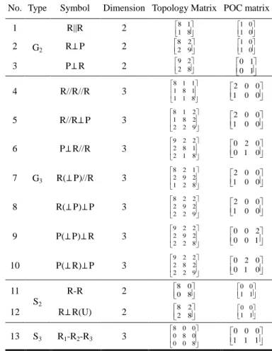
leg. Based on the definition of POC matrix, there are 7 types matrices for 15 sub-chains, as shown in Table 2.

TABLE 2 15 TYPES OF SUB-CHAINS AND THEIR POC

No. Type Symbol Dimension Topology Matrix POC matrix 1 G2 R||R 2 _8 1_{1 8}_   1 0 1 0       2 R⊥P 2 _8_{2 9}2_ 1 01 0       3 P⊥R 2 _9 2_{2 8}_ _0 1_{0 1}_ 4 G3 R//R//R 3 8 1 1 1 8 1 1 1 8         2 0 0 1 0 0       5 R//R⊥P 3 8 1 2 1 8 2 2 2 9         2 0 0 1 0 0       6 P⊥R//R 3 9 2 2 2 8 1 2 1 8         0 2 0 0 1 0       7 R(⊥P)//R 3 8 2 1 2 9 2 1 2 8         2 0 0 1 0 0       8 R(⊥P)⊥P 3 8 2 2 2 9 2 2 2 9         2 0 0 1 0 0       9 P(⊥P)⊥R 3 9 2 2 2 9 2 2 2 8         0 0 2 0 0 1       10 P(⊥R)⊥P 3 9 2 2 2 8 2 2 2 9         0 2 0 0 1 0       11 S2 R-R 2 _8₀ 0₈_ 0 01 1       12 R⊥R(U) 2 _8₂ 2₈_ 0 01 1       13 S3 R1-R2-R3 3 8 0 0 0 8 0 0 0 8         0 0 0 1 1 1      

No. Type Symbol Dimension Topology Matrix POC matrix 14 R1,R2,R3(S) 3 8 5 5 5 8 5 5 5 8         0 0 0 1 1 1       15 R1⊥R2⊥R3 ;R1⊥R3 3 8 2 2 2 8 2 2 2 8         0 0 0 1 1 1      

POC Matrix of legs

Take the leg UP as an example, it contains R1⊥ R2⊥ P3.

Dimension of the output is 3 (2-rotation and 1-translation), and the rotation is around R1 axis and R2 axis, and the translation

along P3 axis. Thus, POC matrix of this leg is M_La 0 0 1 1 1 0

 

 _ _.

Description for PMs and its POC

Description for PMs

To make information concise, a new structural representation of PMs is proposed, which consists of legs and joints on the two platforms.

Firstly, legs of a PM are labeled in turn with the numbers 1~6. Then, all legs are represented using the ordered topology matrix L. Finally, the joints on two platforms are regarded as two correspond virtual legs, expressed by the ordered topology matrices M and B. Therefore, the PM can be described as

PM=(L1, L2, ..., L(v+1), M, B) (10)

The PM in Fig.2(A) has 3-UPS legs and 1-UP leg. The topological structure is PM=(L1,L2,L3,L4,M,B). The joints on

the two platforms are arbitrary.

(A) 3T PM (B) 1T2R PM

FIGURE 2 TWO KINDS OF PMS

The topology matrix Li(i=1~3) for 3-UPS legs and matrix

L4 for UP leg are respectively

i 8 2 0 0 0 0 2 8 0 0 0 0 0 0 9 0 0 0 L 0 0 0 8 2 2 0 0 0 2 8 2 0 0 0 2 2 8                  , 4 8 2 2 L 2 8 2 2 2 9         

Matrix M and B are

8 0 0 0 0 8 0 0 M 0 0 8 0 0 0 0 8            , 8 0 0 0 0 8 0 0 B 0 0 8 0 0 0 0 8            POC matrix of PMs

According to the intersection property of sets, the direction of translation/rotation output of a PM is related to one or more

joints in a certain leg. Thus the No. of this leg should be recorded. So, a column matrix is defined as

1 n 1 pa 1 n 2 t t l M r r l      _ LL   _{  }, (n≤6) (11)

where, l1 and l2 are the No. of the leg specifying the direction of

translation/rotating output, n is the dimension of independent output.

The PM shown in Fig.2(A) has 2-rotation and 1-translation. The POC matrix is pa

0 0 1 4 M

1 1 0 4

   

 _   _{  }, the double 4 indicate that the PM has a translation along P43 joints, and the

directions of rotation are around R41 and R42, both in the fourth

leg.

AUTOMATIC GENERATION OF POC AND DIMENSION OF INDEPENDENT DISPLACEMENT EQUATIONS Automatic POC generation of legs

According to Eq.(3), POC of a leg is the union operation of the POC of all joints. Each leg can be considered as a serial of independent chains and single-DOF joints. Thus, the sub-chains are extracted, and union operation of POCs are mapped to logical “OR” operation of matrices.

For convenience of programming, the POC matrix with dimension less than 6 is supplemented to the same dimension of 2×6 1 2 3 4 5 6 L 1 2 3 4 5 6 t t t t t t M r r r r r r    _ _ (12)

Thus, the POC of a leg can be computed by

3 2 3 2

L G G S S J

POC M( )POC M( M M M M） (13) where, MG3, MG2, MS3, MS2 and MJ are the supplemented forms

of the POC matrices of G3, G2, S3, S2 and single-DOF joints.

Here, based on the topology matrices of legs and the extracted sub-chains and single-DOF joints, the POC of the leg can be generated as follows

① Recognize topology matrix of the leg, and extract G3,

G2, S3, S2 successively.

② Write out the supplemented matrix of G3, G2, S3, S2 and

single-DOF joints.

③ Carry out “OR” operation on supplemented matrices of G3, G2, S3, S2 and single-DOF joints, and obtain the

initial POC matrix of the leg, which denoted as

1 2 3 4 5 6 0 L 1 2 3 4 5 6 t t t t t t M r r r r r r    _ _, 6 0 i r i 1 r =   , 6 0 i t i 1 t =   . ④ Process the translational output generated by parallel

revolute joints.

a. If ξr0>3, then ξr=3 and ξt=ξt0+ξr0-3, and the

translation newly generated lies in the normal plane of the single-DOF or S2 rotational joints.

b. If ξr0 ≤ 3 and ξt0 ≤ 3, the final POC matrix is

Table 1. gives the matrices of four typical legs. Here take the leg P⊥ R//R⊥ R//R as an example.

① Recognize and sequentially extract planar and spherical sub-chains: one G3 sub-chain P⊥ R//R and one G2 planar

sub-chaines R//R.

② Generate the supplemented POC matrix of G3 and G2 as G3 0 2 0 0 0 0 M 0 1 0 0 0 0    _ _, MG2 0 0 0 1 0 0_{0 0 0 1 0 0}  .

③ Carry out “or” operation of MG3 and MG2, and obtain the

POC: ML 0 2 0 1 0 0 = 3 0 0 0 0 0

0 1 0 1 0 0 0 1 0 1 0 0

   

 _  _{ } _ , ξr0=2,

and ξt0=3.

④ ξt0= 3 and ξr0= 2 ,so ML= ML0, that means L

3 0 0 0 0 0 M

0 1 0 1 0 0

 

 _ _, and ξt= 3 indicates that the leg

has three independent translation outputs, ξr=2 indicates

that it has two rotation outputs, r2=r4=1 means the two

rotations are around the axes of R2 and R4 respectively.

Automatic POC generation of PMs

According to Eq.(4), the POC of a PM is the intersection operation on all legs in the PM. Among them, the translational output of the PM is the intersection of translational outputs of all legs, and the same goes for the rotating outputs.

Given two legs L1 and L2, numbered as l1 and l2, the POC

matrices are Li i1 i2 i3 i4 i5 i6 i1 i2 i3 i4 i5 i6 t t t t t t M r r r r r r    _ _ (i=1,2), the

dimension of translation/rotating outputs are ξri=

6 ij j 1 r   and ξti= 6 ij j 1 t   _.

For convenience of description, the translational output of leg i is denoted as Gi=(ξti, ei) and the rotating output as Hi=(ξri,

si), where ei/si are the direction of translational/rotating output

of this leg. If ξti=0/ξri=0, ei/si are Φ(empty set); if ξti=1/ξri=1,

ei/si are spatial lines; if ξti=2/ξri=2, ei/si are plane; if ξti=3/ξri=3,

ei/si are “-”.

Suppose the intersection result is denoted as

1 2 3 4 5 6 L1 L2 1 2 3 4 5 6 t t t t t t M r r r r r r    _ _

I , the dimension of translational/

rotating output is 6 i i 1 r   / 6 i i 1 t 

 respectively. The translational output is G(1∩2)=(ξt, e) and the rotating output is H(1∩2)=(ξr, s),

where e and s are the direction correspond.

Note that the legs L1 and L2, which participate in

computing, can be either the legs constituting the PM or the sub-PM composed by several legs. The POC of PMs can be calculated as follows.

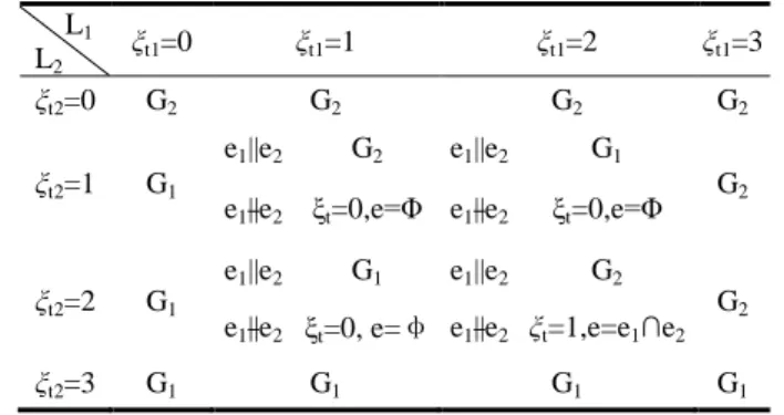
Algorithm for translational output of PMs

The intersection operation of translational output of two legs is to solve G(1∩2)=G1∩G2, which can be obtained according

the rules shown in Table 3.

TABLE 3 INTERSECTION RULES FOR TRANSLATION

L1 L2 ξt1=0 ξt1=1 ξt1=2 ξt1=3 ξt2=0 G2 G2 G2 G2 ξt2=1 G1 e1||e2 G2 e1||e2 G1 G2

e1||e2 ξt=0,e=Φ e1||e2 ξt=0,e=Φ

ξt2=2 G1

e1||e2 G1 e1||e2 G2

G2

e1||e2 ξt=0, e=φ e1||e2 ξt=1,e=e1∩e2

ξt2=3 G1 G1 G1 G1

Algorithms for rotating output of PMs

Similarly, the intersection of rotating output of two POC matrices is to solve H(1∩2)=H1∩H2. The intersection rules are

listed in Table 4.

TABLE 4 INTERSECTION RULES FOR ROTATION

L1 L2 ξr1=0 ξr1=1 ξr1=2 ξr1=3 ξr2=0 H2 H2 H2 H2 ξr2=1 H1 s1||s2 H2 s1||s2 H1 H2 s1||s2 ξr=0,s=Φ s1||s2 ξr=0,s=Φ ξr2=2 H1 s1||s2 H1 s1||s2 H2 H2 s1||s2 ξr=0,s=Φ s1||s2 ξt=1,s=s1∩s2 ξr2=3 H1 H1 H1 H1

Accordance to the analysis above, the flow of generating POC matrices of PMs are as follows

① Input the number of legs, and POC of each leg. ② Intersection operation on translational outputs. ③ Intersection operation on rotating outputs. ④ Output the result of POC of the PM.

Here take the PM of 3-RRC as an example. As shown in Fig.2(B). The topology matrices of legs, joints on the two platforms are described previously.

① Input the number of legs, and POC of each leg. Number of legs is 3, and topology matrices of legs are

i Li i 2 0 0 0 0 0 0 0 0 1 0 0 3 0 0 0 0 0 G M = 1 0 0 0 0 0 0 0 0 0 0 0 1 0 0 0 0 0 H         _{  } _{ } _{  }        (i=1,2,3).

Thus, ξti=3 means arbitrary translation in space, and ξri=1 is

one-dimension rotation around the Ri1 axis in i th

leg, i.e. si=Ri1.

② Intersection operation on translational outputs According to Table 3, ξti= 3, then ξL1t= 3, and G(1∩2)= G2.

③ Intersection operation on rotating outputs

According to Table 4, ξr1=ξr2=ξr3=1, s1=R11, s2=R21, s3=R31

④ Output the result of POC of this PM Mpa=Mpa(1∩2)∩Mb3= 2 G     φ∩ 3₃ G H      = 3 G     φ

The output of 3-RRC PM is 3-translation, and the result is consistent with those in Ref [5].

Calculating the number of independent displacement equations

Eq(6) shows that solving the number of independent displacement equations of an independent loop (SLC) involves the union operation of POC matrices. For the legs L1 and L2

mentioned above, supposing that the result matrix of union is

1 2 3 4 5 6 L1 L2 1 2 3 4 5 6 t t t t t t M r r r r r r   _ _

The dimension of independent output is

ξLr= ξLt=

Translational output is G(1∪2)= (ξLt, e) and rotating output

is H(1∪2)= (ξLr, s), where e/s is the direction of

translation/rotation. Then the number of the independent displacement equations of the independent loop is ξL= ξLt + ξLr.

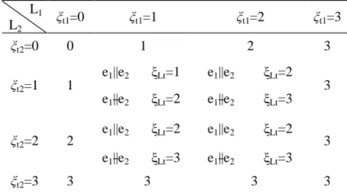
Algorithms for the dimension of translation output of SLC

Solving the dimension of translational output of a SLC is essentially to calculate ξLt=dim(G1∪G2), whose operation rules

are shown in Table 5.

TABLE 5. ALGORITHMS FOR THE DIMENSION OF TRANSLATIONAL OUTPUT L1 L2 ξt1=0 ξt1=1 ξt1=2 ξt1=3 ξt2=0 0 1 2 3 ξt2=1 1 e1||e2 ξLt=1 e1||e2 ξLt=2 3 e1||e2 ξLt=2 e1||e2 ξLt=3 ξt2=2 2 e1||e2 ξLt=2 e1||e2 ξLt=2 3 e1||e2 ξLt=3 e1||e2 ξLt=3 ξt2=3 3 3 3 3

Similarly, the dimension of rotating output of a SLC is to calculate ξLr=dim(H1∪H2), and its operation rules are shown in

Table 6.

TABLE 6. ALGORITHMS FOR THE DIMENSION OF ROTATING OUTPUT L1 L2 ξt1=0 ξt1=1 ξt1=2 ξt1=3 ξt2=0 0 1 2 3 ξt2=1 1 s1||s2 ξLr=1 s1||s2 ξLr=2 3 s1||s2 ξLr=2 s1||s2 ξLr= ξt2=2 2 s1||s2 ξLr=2 s1||s2 ξLr=2 3 s1||s2 ξLr=3 s1||s2 ξLr=3 ξt2=3 3 3 3 3

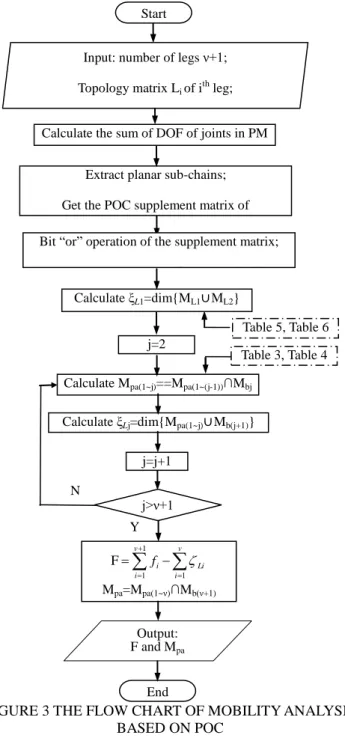
PROCEDURE OF AUTOMATIC MOBILITY ANALYSIS OF PMS

Based on the algorithm for POC of legs and PMs and for the number of the independent displacement equations, the mobility analysis flow for PMs is established as shown in Fig.3. Step1. Input topological structure of the PM.

Input topology matrices L1, …, L(ν+1) and number leg in

sequence automatically, and input the axis relation matrix M and B on the moving platform and fixed platform. Obtain the number of the joints fi and the

number of ν+1 legs.

Step2. Calculate (ν+1) POC matrix of legs: ML1,...ML(ν+1).

Step3. Calculate the sum of all joints in the PM: f(1~(ν+1))= +1 i 1 f i    . Step4. Calculate the number of the independent displacement

equations of the 1st loop SLC1: ξ1

① Calculate the dimension of the independent translational output of SLC1: ξL1t= dim(G1∪G2).

② Calculate the dimension of te independent rotating output of SLC1: ξL1r= dim(H1∪H2).

③ Calculate ξL1= ξL1t+ξL1r.

Step5. Calculate the POC matrix MP(1∩2) of the sub-PM P(1-2)

composed by the 1th and 2th legs.

① Calculate the translational output G(1∩2)=G1∩G2.

② Calculate the rotating output H(1∩2)=H1∩H2.

③ Get 1 2 (1 2) 1 2 G MP H       _ ( )_ ( ) .

Step6. Calculate the POC matrix Mpa(1~j)= Mpa(1~(j-1))∩Mbj of the

sub-PM P(1-j) composed by the front j th

(j=3,...,ν) legs. Step7. Calculate the number of the independent displacement

equations of the jth (j=2,...,ν) independent loop SLCj: ξj=dim(Mpa(1~j)∪Mb(j+1)).

Step8. Calculate the number of DOF: _{1~(ν+1)} ν _i

i=1

F=f -ξ .

Step9. Determine the property of mobility of this PM: Mpa=Mpa(1-ν)∩ML(ν+1) . 6 i i 1 r   6 i i 1 t  

FIGURE 3 THE FLOW CHART OF MOBILITY ANALYSIS BASED ON POC

SOFTWARE IMPLEMENTATION AND CASE STUDY Software implementation

According to the basin principle discussed above, an automatic mobility analysis platform for PMs was developed by VC++ 6.0. Using the platform, large number of PMs listed in [6] have been analyzed automatically based on the input of topology matrix and results have proved the validity of the software.

The input information mainly includes the number of legs and topology matrix. Using decimal array and easy to operate.

The analysis results include the DOF, the dimension of the independent translational/rotating output of the moving platform, and their corresponding axis direction.

Case study

Detailed examples of mobility analysis of two PMs are presented in this section.

Mobility analysis of the Tricept PM

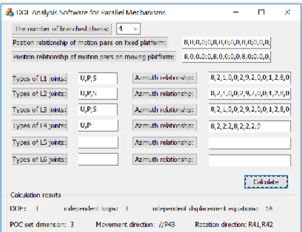
The PM of Tricept shown in Fig.2(A) has 3 DOF which is one translation and two rotation. The legs are 3-UPS and 1-UP. The axes of joints on the two platforms are of general.

(1) Input topological structural matrices of the PM

Topology matrix of UPS leg is i

8 2 1 0 0 2 9 2 0 0 L 1 2 8 0 0 0 0 0 8 5 0 0 0 5 8                , (i=1~3).

Topology matrix of UP leg is 4

8 2 2 L 2 8 2 2 2 9          .

To the two virtual legs on the platforms, topology matrices M and B are 8 0 0 0 0 8 0 0 M 0 0 8 0 0 0 0 8            , 8 0 0 0 0 8 0 0 B 0 0 8 0 0 0 0 8            . Number of legs ν+1=4

(2) Calculate POC matrix of legs ML1,...ML4.

① i Li i 3 0 0 0 0 0 G M = 3 0 0 0 0 0 H      _   _{  }, ξir=3, and ξit=3 (i=1~3) ② 4 L4 4 0 0 1 0 0 0 G M = 1 1 0 0 0 0 H      _   _{  },and ξ4t=1, ξ4r=2.

(3) Get the sum of all joints in this PM: f(1-4)=6+6+6+3=21.

(4) Calculate the number of the independent displacement equations of the first loop (SLC1)

① ξti=3, as shown in Table 5, ξL1t=3, G(1∪2)=G2 (i=1,2).

② ξri=3, then ξL1r=3, H(1∪2)=H2 (i=1,2).

③ So, ξL1=ξL1t+ξL1r=3+3=6.

(5) Calculate the POC matrix MP(1∩2) of sub-PM constituted by

1st and 2nd legs.

① ξti=3, as shown in Table 3, G(1∩2)=G2 (i=1,2).

② ξri=3, as shown in Table 4, H(1∩2)=H2 (i=1,2).

③ So, 2 (1 2) 2 G MP H    _ _.

(6) Calculate the POC matrix of sub-PM composed by the front three legs: Mpa(1~3)= Mpa(1~2)∩Mb3= 2 3 3

2 3 G G G = H H H                  3 ∩ .

(7) Calculate the number of the independent displacement equations of SLC2: ξL2=dim(Mpa(1~2)∪Mb3).

① ξt(1∩2)=3, and ξt3=3, then ξL2t=3.

② ξr(1∩2)=3, and ξr3=3,then ξL2r=3.

③ then, ξL2=ξL2t+ξL2r=3+3=6.

Y N

Calculate Mpa(1~j)==Mpa(1~(j-1))∩Mbj

j>ν+1 j=j+1

Calculate ξLj=dim{Mpa(1~j)∪Mb(j+1)}

End Output: F and Mpa





Get the POC supplement matrix of sub-chains, and single-DOF joints.

Start

Calculate ξL1=dim{ML1∪ML2}

Input: number of legs ν+1; Topology matrix Li of ith leg;

Topology matrix M and B on two platforms. Calculate the sum of DOF of joints in PM

j=2

Bit “or” operation of the supplement matrix; Calculating the POC Mbi (i=1,…,ν+1) of leg.

Similarly, the number of the independent displacement equations of SLC3 is ξL3=ξL3t+ξL3r=3+3=6.

(8) Get the number of DOF: _{ 1~4} 3 _i

i 1

F=f - =21- 6+6+6 =3



 ( ) . (9) Get the property of mobility:

Mpa=Mpa(1-3)∩Mb4= 3 G H      3∩ 4 G H      4= 4 G H      4.

The results show that this mechanism has 1T2R output, the rotating directions are around R41 and R41, and the translational

direction along P43 joint. The result generated by software is

shown in Fig.4, which is consistent with those in Ref.[6].

FIGURE 4. MOBILITY ANALYSIS OF TRICEPT

Mobility analysis of a 3-RRC PM

Fig.2(B) shows a 3-RRC PM. It has three identical RRC legs connecting the two platforms, labeled with the number 1~3. The topological structure of this PM is PM=(L1,L2,L3,M,B). The fixed platform is a triangle, and axes

of the joints on the two platforms are all coplanar. (1) Input topology matrices of the PM

Topology matrix of RRC leg is i

8 1 1 1 1 8 1 1 L 1 1 8 1 1 1 1 9            , (i=1~3).

To two virtual legs on the platforms, topology matrices M and B are 9 5 5 M 5 9 5 5 5 9          and 8 5 5 B 5 8 5 5 5 8          . Number of legs ν+1=3.

(2) Calculate POC matrix of legs ML1,...ML3.

① Recognize and sequentially extract planar and spherical sub-chains: one G3 sub-chain R//R//R and one

single-DOF P joint.

② Generate the POC supplemented matrices of G3 and P

as G3 2 0 0 0 0 0 M 1 0 0 0 0 0    _ _ and P 0 0 0 1 0 0 M 0 0 0 0 0 0    _ _.

③ Carry out “OR” operation on POC matrices of all legs

Li 2 0 0 1 0 0 3 0 0 0 0 0 M = 1 0 0 0 0 0 1 0 0 0 0 0      _  _{ } _, ξr0=1, and ξt0=3 (i=1~3)

④ ξt=3 and ξr=1, then ML=MLa0, that means Li

3 0 0 0 0 0 M

1 0 0 0 0 0

 

 _ _, and ξit=3 indicate that the leg has three

translational output along arbitrary direction, ξir=1 indicates

that it has one rotating output, ri1=1 means that the rotation is

around the axes of Ri1, i.e. si=Ri1.

i Li i 3 0 0 0 0 0 G M = 1 0 0 0 0 0 H      _   _{  }

(3) Calculate the sum of all joints in this PM: f(1-3)=4+4+4=12.

(4) Calculate the number of the independent displacement equations of the first loop (SLC1)

① ξti=3, as shown in Table 5, ξL1t=3 (i=1,2).

② ξri=1, and s1||s2, then, ξL1r=2 (i=1,2).

③ So, ξL1=ξL1t+ξL1r=3+2=5.

(5) Calculate the POC matrix MP(1∩2) of sub-PM constituted by

the 1st and 2nd legs

① ξti=3, as shown in Table 3, G(1∩2)=G2 (i=1,2).

② ξri=1, and s1||s2,as shown in Table 4, H(1∩2)=Φ (i=1,2).

③ So, 2

(1 2)

G MP     

φ.

(6) Calculate the POC matrix of PM constituted by the front three legs: Mpa(1~3)=Mpa(1~2)∩ML3=G2

φ∩ 3 G H      3 =G3   φ.

(7) Calculate the number of the independent displacement equations of SLC2: ξL2=dim(Mpa(1~2)∪Mb3)

① ξt3=3, as shown in Table 3, ξL2t=3.

② ξr(1-2)=0, and ξr3=1,as shown in Table 4, ξL2r=1.

③ Thus, ξL2=ξL2t+ξL2r=3+1=4.

(8) Get the number of DOF: _{ }

3 i 1~3 1 F=f - =12- 5+4 =3 i    ( )

(9) Get the property of mobility: Mpa=Mpa(1-3)=_G3_ φ.

It shows that this PM has 3 DOF, three translation. The result automatically generated shown in Fig.5. The result is consistent with those in Ref[5].

CONCLUSIONS

A matrix description for mapping the topological structure with POC of legs and PMs was established. It includes not only the type and size of the translational/rotary output, but also represents the orientation of the output axis. By extracting the planar and spherical sub-chains orderly, the POC of a leg can be transformed into the logical "OR" operation of the matrices. An algorithm for POC of a PM was established without manual intervention. Algorithm of mobility analysis automatically of PMs is proposed. Software for mobility analysis of PMs was created and typical examples were provided in detail to show its effectiveness.

ACKNOWLEDGMENTS:

This research is sponsored by the NSFC (Grant No. 51475050).

REFERENCES

[1] HUANG Zhen, ZHAO Tieshi, Advanced Spatial Mechanism[M]. Beijing: Higher Education Press, 2006. [2] Kong X W, Gosselin C M, Type Synthesis of 3-DOF

Parallel Manipulators Based on Screw Theory, Journal of Mechanical Design, 2004,126(1):83-92.

[3] DAI Jiansheng. Spatial Algebra and Lie Algebra[M]. Beijing: Higher Education Press, 2014.

[4] Rico J M, Gallardo J, Ravani B. Lie Algebra and the Mobility of Kinematic Chains[J]. Journal of Robotic Systems, 2003, 20(8):477-499.

[5] HERVE, J. M. The Lie Group of Rigid Body Displacements, a Fundamental Ttool for Mechanism Design[J]. Mechanism & Machine Theory, 1999, 34(5):719-730.

[6] YANG Tingli, LIU Anxin, et al. Theory and Application of Robot Mechanism Topology[M]. Beijing: Science Press, 2012.

[7] SHEN Huiping, YIN Hongbo, LI JU, et al. Position and Orientation Characteristic Based Method and Enlightenment for Topology Characteristic Analysis of Typical Parallel Mechanisms and Its Application[J]. Journal of Mechanical Engineering, 2015, 51(13):101-115.

[8] Chai Xinxue, Research on the Aanalysis Method of DOF of Parallel Mechanism in the Framework of Geometric Algebra[D].Zhejiang University of Technology, 2017. [9] CAO Wenao. Digital Type Synthesis Theory of Spatial

Multi-Loop Coupled Mechanisms[D]. Yanshan University, 2014.

[10] LIAO Ming, LIU Anxin, SHEN Huiping, et al. Symbolic Derivation of Position and Orientation Characteristics of Parallel Mechanisms[J]. Transactions of the Chinese Society for Agricultural Machinery, 2016, 46(3):395-404. [11] Ding H, Cao W, Cai C, et al. Computer-aided Structural

Synthesis of 5-DOF Parallel Mechanisms and the Establishment of Kinematic Sstructure Databases[J].