Pixel Classification using General Adaptive Neighborhood-based Features

HAL Id: hal-01070876

https://hal.archives-ouvertes.fr/hal-01070876

Submitted on 13 Oct 2014

HAL is a multi-disciplinary open access

archive for the deposit and dissemination of

sci-entific research documents, whether they are

pub-lished or not. The documents may come from

teaching and research institutions in France or

abroad, or from public or private research centers.

L’archive ouverte pluridisciplinaire HAL, est

destinée au dépôt et à la diffusion de documents

scientifiques de niveau recherche, publiés ou non,

émanant des établissements d’enseignement et de

recherche français ou étrangers, des laboratoires

publics ou privés.

Pixel Classification using General Adaptive

Neighborhood-based Features

Víctor González-Catro, Johan Debayle, Vladimir Ćurić

To cite this version:

Víctor González-Catro, Johan Debayle, Vladimir Ćurić. Pixel Classification using General Adaptive

Neighborhood-based Features. 22nd International Conference on Pattern Recognition, Aug 2014,

Stockholm, Sweden. pp. 3750-3755, �10.1109/ICPR.2014.644�. �hal-01070876�

Pixel Classification using General Adaptive

Neighborhood-based Features

V´ıctor Gonz´alez-Castro, Johan Debayle

´

Ecole Nationale Sup´erieure des Mines de Saint- ´Etienne LGF UMR CNRS 5307

42023 Saint-Etienne Cedex 2, FRANCE Email: [email protected], [email protected]

Vladimir ´

Curi´c

Centre for Image Analysis Uppsala University

Uppsala, Sweden Email: [email protected]

Abstract—This paper introduces a new descriptor for charac-terizing and classifying the pixels of texture images by means of General Adaptive Neighborhoods (GANs). The GAN of a pixel is a spatial region surrounding it and fitting its local image structure. The features describing each pixel are then region-based and intensity-region-based measurements of its corresponding GAN. In addition, these features are combined with the gray-level values of adaptive mathematical morphology operators using GANs as structuring elements. The classification of each pixel of images belonging to five different textures of the VisTex database has been carried out to test the performance of this descriptor. For the sake of comparison, other adaptive neighbor-hoods introduced in the literature have also been used to extract these features from: the Morphological Amoebas (MA), adaptive geodesic neighborhoods (AGN) and salience adaptive structuring elements (SASE). Experimental results show that the GAN-based method outperforms the others for the performed classification task, achieving an overall accuracy of 97.25% in the five-way classifications, and area under curve values close to 1 in all the five ”one class vs. all classes” binary classification problems.

Keywords—Pixel description; adaptive neighborhoods; Minkowski functionals; morphometrical functionals; adaptive mathematical morphology.

I. INTRODUCTION

The so-called General Adaptive Neighborhood Image Pro-cessing (GANIP) approach has been developed by Debayle and Pinoli [1] for the adaptive processing and analysis of gray-level images. In this framework an image is represented as a set of adaptive neighborhoods (i.e. a surrounding region for each pixel, fitting its local spatial structures). Mathematically, a General Adaptive Neighborhood (GAN) is a connected component whose point intensity values (measured in relation to a certain criterion such as luminance, contrast, etc.) fit within a specific range of homogeneity tolerance. It makes GAN adaptive with respect to the spatial structures and defined from the gray-level image itself. Thereafter, GANs can be used as operational windows for adaptive image processing and analysis. For example, these GANs have been used as struc-turing elements for adaptive mathematical morphology [2]. In addition, geometrical and morphometrical measurements of GANs have also been used for characterizing gray-level images [3], [4].

In the literature, other adaptive neighborhoods have been proposed for image processing. Lerallut et al. introduced the concept of morphological amoebas (for defining mor-phological operators) whose shape is locally adapted to the

image contour variations by means of a weighted geodesic distance [5]. Grazzini and Soille also proposed a filtering approach based on adaptive neighborhoods obtained by means of a geodesic distance criterion [6] which achieved an edge-preserving smoothing. Recently, ´Curi´c et al. presented the salience adaptive structuring elements, that vary both their shape and size according to the salience of edges in the image [7]. Note that all these adaptive neighborhoods have been mostly used as adaptive structuring elements in morphological operators.

The purpose of this paper is to characterize and classify pixels of texture images. In order to describe them, some local information around the pixels are taken into account. In this way, region-based and intensity-based measurements of the GANs (which fit to the local image structures) are used as pixel descriptors. More precisely, the features describing each pixel are geometrical (using Minkowski functionals [3]) and morphometrical functionals [4] of its corresponding GAN. These features are combined with the gray-level values of GAN-based adaptive morphological operations of the image at that point. Therefore, these descriptors characterize both the geometry, morphometry and intensities of local structures surrounding the pixels. For the sake of comparison, this de-scriptors have also been computed from Morphological Amoe-bas [5], Adaptive Geodesic Neighborhoods [6], and Salience Adaptive Structuring Elements [7].

The paper is organized as follows: First, a brief review of the General Adaptive Neighborhood Image Processing (GANIP) framework is made in section II. Thereafter, some theoretical aspects of the proposed descriptor are given in section III. Section IV depicts a summary of the other adaptive neighborhoods, and then the experimental framework and results are presented in section V. Finally, the conclusions are presented in section VI.

II. GENERALADAPTIVENEIGHBORHOODIMAGE

PROCESSING(GANIP)

The GANIP approach [1] provides a general framework for multiscale, local and adaptive image processing and analysis of gray-level images. It is based on extracting spatial neigh-borhoods called General Adaptive Neighneigh-borhoods (GANs) from the points of the image as the size and shape of the neighborhoods are adapted to the local features of the image. Specifically, a GAN is a subset of the spatial support D ⊆ R2

constituted by connected points whose values in relation to a selected criterion (luminance, contrast,...) fit within a homo-geneity tolerance. As a result, GANs are adaptive with the spatial structures and defined from the gray-level image itself. Let f be an image defined in D with range in R, and let h be a criterion mapping, also defined in D and valued in R, based on local measurements such as luminance, contrast, etc. For each point x ∈ D, the GANs (denoted Vmh(x)) are subsets in D built upon h in relation to a homogeneity tolerance m ∈ R+. More precisely, Vmh(x) fulfills two conditions:

• The measurement of the criterion mapping of its points is close to the one of x

∀y ∈ Vh

m(x), |h(y) − h(x)| ≤ m

• The GAN is a path-connected set (according to the usual Euclidean topology on D ⊆ R2₎

Thus, the GANs are formally defined as:

V_mh(x) = C_{{y∈D: |h(y)−h(x)|≤m}}(x) (1) where CX(x) denotes the path connected component of X ⊆ D containing x ∈ D. Therefore, it is ensured that ∀x ∈ D x ∈ Vm(x).h

However, these GANs do not satisfy the symmetry property, defined as:

∀ x, y ∈ D y ∈ A(x) ⇐⇒ x ∈ A(y) (2) where {A(x)}x∈D is a collection of subsets A(x) ⊆ D. For this reason, GANs defined in equation (1) are called Weak General Adaptive Neighborhoods (W-GANs).

In order to get this property satisfied, a new set of GANs, called Strong General Adaptive Neighborhoods (S-GANs) is defined as: Nmh(x) = [ z∈D {Vmh(z) : x ∈ V h m(z)}. (3)

The reader interested in further theoretical aspects on GANs is referred to [1].

III. GAN-BASED DESCRIPTOR

As it has been previously pointed out, each pixel will be described by means of geometrical and morphometrical functionals computed from its corresponding GAN, combined with the gray-level of the results of some GAN-based adaptive morphological operations at that point. This section explains these methods.

A. GAN-based Minkowski functionals

Integral geometry provides a suitable family of geometrical and topological descriptors of 2-D and 3-D spatial patterns, known as Minkowski functionals [8]. In 2-D, there are three Minkowski functionals: area, perimeter and Euler number, denoted respectively A, P and χ.

These functionals are defined on the class of nonempty compact convex sets in R2. They have been extended to the convex ring [9], i.e. the set of all finite unions of convex bodies,

which may be considered as a realistic Euclidean model for digital images.

In this paper the densities of these functionals are used, (i.e. the ratios of the intensities and the area of the spatial support D). The density of the area, perimeter and Euler number are denoted AA, PA and χA, respectively.

The GAN-based Minkowski maps [3] are defined by as-signing to each point x ∈ D the Minkowski density functional Vh

m(x). More explicitly, the GAN-based Minkowski map of a gray-level image, denoted by µhm, is defined by:

µh_m(x) = µ(V_mh(x)) (4) where µ denotes a Minkowski density functional (i.e. µ ≡ AA, µ ≡ PA or µ ≡ χA).

B. GAN-based morphometrical functionals

For a simply connected compact set in R2_{, the relationships} between the six geometrical functionals area (A), perimeter (P ), radii of the inscribed and circumscribed circles (r and R respectively) and the minimum and maximum Feret diameters (ω and d, respectively) are constrained by some geometric inequalities. Some of these inequalities are restricted to convex sets.

The inequalities that link geometrical functionals by pairs actually determine the so-called extremal connected compact sets, which are the sets for which the inequalities become equalities. Furthermore, they allow to determine morphome-trical functionals, which are invariant under similitude trans-formations and, therefore, do not depend on the global size of the compact set. Morphometrical functionals are defined as ratios between the corresponding geometrical functionals in which the units are dimensionally homogeneous, so the result is dimensionless. Moreover, a normalization by a constant value leave those ratios in the interval [0, 1].

The inequalities between geometrical functionals along with the corresponding morphological functionals and ex-tremal connected compact sets are shown in table I. It is necessary to point out that these inequalities are not restricted to convex sets. The extremal sets shown in this table are disks (C), line segments (L), the constant width compact sets (W), compact sets of diameter d containing an equilateral triangle of side-length d (Z), simply connected compact sets (Y) and some compact convex sets (X).

The morphometrical functionals can be classified according to their concrete meanings:

• Roundness: 4πA/P2_{, 4A/πd}2_{, πr}2_{/A, A/πR}2 • Circularity: 2πr/P , r/R, 2r/d, ω/2R

• Diameter constancy: πω/P , ω/d • Thinness: 2d/P , 4R/P

In addition, the functional √3R/d expresses both the equilateral triangularity and the diameter constancy. The ratios 2r/ω and d/2R do not have a concrete meaning, and they are equal to one for many compact sets.

Similar to what was done with the Minkowski maps, adaptive morphometrical maps of an image can be defined [4]

TABLE I. INEQUALITIES BETWEEN GEOMETRICAL FUNCTIONALS AND THE CORRESPONDING MORPHOMETRICAL FUNCTIONALS,NOT

RESTRICTED TO COMPACT CONVEX SETS.

Geometrical functionals Inequalities Morphological functionals Extremal sets r, R r ≤ R r/R C ω, R ω ≤ 2R ω/2R C A, R A ≤ πR2 _A/πR2 _C d, R d ≤ 2R d/2R Y r, d 2r ≤ d 2r/d C ω, d ω ≤ d ω/d W A, d 4A ≤ πd2 4A/πd2 C R, d √3R ≤ d √3R/d Z r, P 2πr ≤ P 2πr/P C ω, P πω ≤ P πω/P W A, P 4πA ≤ P2 4πA/P2 C d, P 2d ≤ P 2d/P L R, P 4R ≤ P 4R/P L r, A πr2≤ A πr2/A C r, ω 2r ≤ ω 2r/ω X

by assigning to each point x the corresponding morphometrical functional of the GAN of that point.

The reader interested in further theoretical details about ge-ometrical and morphge-ometrical functionals of GANs is referred to [3], [4].

C. GAN-based mathematical morphology

Mathematical Morphology is a theory developed from the ideas of Matheron [10] and Serra [11] for binary images, and generalized to gray-level images later [12]. The two fundamental morphological operators are erosion and dilation, defined respectively as:

EB(f (x)) = inf{f (w) : w ∈ B(x)} (5) DB(f (x)) = sup{f (w) : w ∈ ˇB(x)} (6) where B(x) denotes the structuring element B whose origin is located at point x, and ˇB(x) stands for the reflection of B, i.e. ˇB(x) = {z ∈ D : x ∈ B(z)}.

The idea behind the General Adaptive Neighborhood Math-ematical Morphology (GANMM) [1], [2] is to substitute the usual structuring elements by the adaptive ones at each pixel of the image.

The S-GANs (see equation (3)) are autoreflected subsets (a subset A(x) is autoreflected if and only if ˇA(x) = A(x), ∀x ∈ D), which have been used as adaptive structuring ele-ments for GANMM. Therefore, GAN-based adaptive erosion and dilation can be expressed as:

Ehm(f )(x) = inf w∈Nh m(x) (f (w)) (7) D_mh(f )(x) = sup w∈Nh m(x) (f (w)) (8)

Thereafter, more advanced adaptive morphological op-erators can be defined (e.g. openings, closings, alternating sequential filters, etc.) [2].

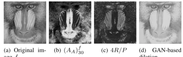
An example of a Minkowski functional map, a morphome-trical functional map and the adaptive dilation of an image is shown in Fig. 1.

(a) Original im-age f

(b) (AA)f30 (c) 4R/P (d) GAN-based

dilation

Fig. 1. Examples of the GAN-based Minkowski map of the area, AA,

(b), GAN-based morphometrical functional map 4R/P (c) and GAN-based dilation (d). The GANs were computed with respect to the luminance criterion (h ≡ f ) using a homogeneity tolerance m = 30. Each pixel is then described by geometrical, morphometrical and intensity features.

IV. OTHER ADAPTIVE NEIGHBORHOODS

Other adaptive neighborhoods defined in the literature will be used to compute the Minkowski and morphometrical func-tionals and as adaptive structuring elements in morphological operations. The aim is to compare the resulting descriptors with the GAN-based ones in the pixel classification task. These adaptive neighborhoods are the Morphological Amoebas (MA) [5], the Adaptive Geodesic Neighborhoods (AGN) [6] and the Salience Adaptive Structuring Elements [7] (SASE).

A gray-level image f can also be represented as a surface S with two spatial coordinates in D and other coordinate corresponding to the intensity value of the image at these co-ordinates. The geodesic distance between two points (x, f (x)) and (y, f (y)) on S is the minimum cost to travel from one to the other along the surface. Since digital images are considered in this paper, discrete paths have been used.

Let Pxy be a geodesic path connecting x and y. It can be considered as a set {x1, x2, ..., xn+1} with x1 = x and xn+1 = y. The cost of the geodesic path connecting two adjacent points, c(xi, xi+1), i ∈ {1, 2, ..., n}, should take into account both (a) the spatial distance between xi and xi+1 and (b) the distance between their corresponding gray-level values f (xi) and f (xi+1). The cost, C, of the path Pxy is

C(Pxy) = n X i=1

c(xi, xi+1)

and the geodesic distance between x and y is d(x, y) = min

Pxy

C(Pxy). (9)

Keeping this in mind, the next sections briefly present how amoebas, AGNs and SASEs are defined and how these costs are computed for each method.

A. Morphological Amoebas

As it is defined in [5], a morphological amoeba centered in x ∈ D is:

Ar(x) = {y ∈ D : d(x, y) < r} (10) where r is the so-called radius of the amoeba.

For this method the cost between two adjacent points is defined by:

where λ > 0.

In this work the considered discrete spatial distance kxi− xi+1k_Z2 is the h3, 4i distance, and λ = 0.25, as done in [7].

B. Adaptive Geodesic Neighborhoods

Grazzini and Soille use the same principle for their locally Adaptive Geodesic Neighborhoods [6], but they propose two different ways of computing the cost. The first one is called the ∆-time, which is defined as:

c(xi, xi+1) =1

2|f (xi) − f (xi+1)| · kxi− xi+1kZ2 (12) where the h3, 4i distance has been considered as the discrete spatial distance kx − yk_Z2 [7].

The second one is called the Σ-time. The difference with the ∆-time is that the image gradient ∇f is used instead of the image itself f .

Both cost functions have been assessed for this particular application, and it was found that the ∆-time outperformed the Σ-time in terms of classification accuracy. Therefore, the results shown in this paper have been achieved using the cost function defined in equation (12).

C. Salience Adaptive Structuring Elements ´

Curi´c et al. proposed other adaptive structuring elements, obtained by computing the distances between the points using the Salience Distance Transform (SDT) [7], thus, weighting the edges of the image by their importance, or salience.

To compute the Salience Map (SM) of the image, first of all, the edges in the input image are extracted using the gradient estimation and the non-maximal suppression from the Canny edge detector. Let NMS(f ) be the resulting ”edge im-age”. Then, the Salience Distance Transform [13] is computed taking −NMS(f ) as input, getting non-zero values for the edge pixels. Finally, the Salience Maps (SM) are the inverted values of the SDT shifted to positive values. Therefore, the highest values in SM correspond to the strongest edges in the images. Finally, the SM can be written in the following mathematical formulation:

SM(y) = Offset + sup x∈D

{NMS(f )(x) − kx − yk_Z2}, (13)

where y ∈ D and Offset = infy∈Dsup_x∈D{NMS(f )(x) − kx−yk_Z2}. Once again, the considered discrete spatial distance

kx − yk_Z2 is the h3, 4i distance.

Thereafter, the cost of the path between adjacent points is defined as:

c(xi, xi+1) = SM(xi) + SM(xi+1). (14) Finally, the salience adaptive structuring element (SASE) with origin at x is defined as:

Sr(x) = {y : d(x, y) < r} (15) where d(x, y) is computed using equation (9).

In this case the radii of the SASEs are spatially variant: the higher the value of a point on the SM, the closer it is to a salient edge and thus, its corresponding structuring element

(a) FaBa (b) FaWo (c) FoBe (d) FoSw (e) Stone Fig. 2. Examples of used the VisTex sub-categories with their names.

should have a smaller radius. In this paper the maximum of the SM is used to derive the radii of the SASEs, therefore:

r(x) = k · max(SM) − SM(x) (16) where k ≥ 1 is a parameter that regulates the size of the SASEs.

V. EXPERIMENTS AND RESULTS

This section presents the pixel classification in gray-level textures. Concretely, each pixel has been described by means of some features (region-based and intensity-based) computed from its corresponding adaptive neighborhood (of different sizes). Afterwards, this feature vector has been classified by means of a neural network, so the pixel is assigned to a class. The next sections describe the images, descriptors, classification stage and results.

A. Texture database

Five different classes have been extracted from the MIT VisTex1 _{database. Textures in this database are taken from} different materials and divided into several categories. Within some of them there are different sub-categories, so they have been divided as it was done in [14].

Each original image has a spatial resolution of 512 × 512 pixels, and was divided into 25 sub-images of 102 × 102 pixels, with no overlapping among themselves. Thereafter, five images were randomly chosen from each class to be used in the experiment (i.e. 25 images are used in the experiment). It may seem the number of images is not enough for a classification task, but it is necessary to remember that the classification is not carried out on the images but on the pixels. Therefore, the dataset has 25 × 102 × 102 = 260100 elements. In Fig. 2 a sub-image from each of the classes that have been used is shown.

B. Pixel-level description

Each pixel of the image is characterized by a feature vector constructed by a concatenation of (i) the mean and standard deviation of the Minkowski density functionals (AA, PA and χA) of adaptive neighborhoods of different sizes whose origin is placed at that pixel (i.e. 6 features), (ii) the mean and standard deviation of the 15 morphometrical functionals shown in table I of the same adaptive neighborhoods (i.e. 30 features) and (iii) the gray-level values of the considered point in the original image and the corresponding adaptive erosions and dilations using adaptive neighborhoods with increasing sizes as structuring elements.

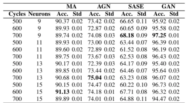
TABLE II. MEAN AND STANDARD DEVIATION OF THE ACCURACY OVER THE10CLASSIFICATIONS FOR THE DIFFERENT SCENARIOS OF

NEURONS IN THE HIDDEN LAYER/TRAINING CYCLES.

MA AGN SASE GAN Cycles Neurons Acc. Std Acc. Std Acc. Std Acc. Std

500 9 90.37 0.02 73.42 0.02 66.65 0.11 95.92 0.02 600 9 89.93 0.01 72.87 0.02 60.65 0.09 95.58 0.02 700 9 89.74 0.02 74.08 0.03 68.18 0.09 97.25 0.01 500 11 89.93 0.01 73.00 0.02 63.44 0.07 96.39 0.01 600 11 89.60 0.02 72.89 0.02 61.52 0.08 96.19 0.02 700 11 89.75 0.01 73.67 0.03 62.53 0.08 96.43 0.02 500 13 90.17 0.01 72.39 0.03 64.17 0.09 95.40 0.02 600 13 89.85 0.01 73.44 0.02 64.46 0.07 95.64 0.03 700 13 90.68 0.01 75.04 0.02 63.23 0.08 96.07 0.02 500 15 90.15 0.01 74.47 0.02 60.22 0.10 96.73 0.02 600 15 91.13 0.02 74.18 0.01 67.71 0.08 96.32 0.02 700 15 89.89 0.01 74.01 0.01 64.88 0.11 94.47 0.02

The adaptive neighborhoods have been computed from the images themselves (e.g. h ≡ f in GANs). In order to make the size of the neighborhoods vary, different values for the tolerance m in the case of the GANs, radius r for the amoebas or AGNs or the parameter k for the SASEs (see eq. (16)) have been used. Several values for these parameters have been tested for all methods, but the best results have been achieved for values from 5 to 100 in steps of 5 (i.e. 20 different values). Therefore, each pixel is described by a vector of 77 features.

C. Classification

All these descriptors have been classified using a feed-forward Artificial Neural Network [15] with one hidden layer, and softmax activation function in the hidden and output layers (to guarantee that outputs satisfy the probability constraints) [16].

The learning of the network has been carried out using momentum and adaptive learning rate algorithm. Different combinations of training cycles and neurons in the hidden layer have been used, in order to assess the impact of this configuration in the results. Concretely, 9, 11, 13 and 15 neurons and 500, 600 and 700 cycles have been used.

The training have been carried out using the descriptors of the pixels of 3 images per class (chosen randomly) and the pixels of the other 2 have been used as test set. This process has been repeated during 10 times, to avoid possible random effects in the classification. Data were normalized previous to classification, so that they have zero mean and standard deviation equals to one.

D. Results

The mean and standard deviation of the accuracy (i.e. the ratio of well classified pixels), in %, over the 10 classification iterations are shown in table II, for the different classification scenarios (i.e. neurons in the hidden layer/training cycles). The first row shows the different types of adaptive neighborhoods that have been tested i.e., Morphological Amoebas (MA), Adaptive Geodesic Neighborhoods (AGN), Salience Adaptive Structuring Elements (SASE) and the general adaptive neigh-borhoods (GAN).

First of all, it is remarkable the good performance of the descriptor based on the GANs compared to the other methods:

TABLE III. AREA UNDER THEROCCURVES OF THE CLASSIFIER GENERATED BY EACH DESCRIPTOR FOR EACH BINARY PROBLEM

MA AGN SASE GAN FaBa vs. non-FaBa 0.9781 0.9561 0.9552 0.9972 FaWo vs. non-FaWo 0.9948 0.9279 0.9222 0.9996 FoBe vs. non-FoBe 0.9884 0.8832 0.8807 0.9955 FoSw vs. non-FoSw 0.9788 0.9613 0.9599 0.9987 Stone vs. non-Stone 0.9962 0.9597 0.9547 0.9997

they achieve a maximum accuracy of 97.25% (with a neural network configuration of 9 neurons in the hidden layer and 700 training cycles), whereas the descriptors based on MAs, AGNs and SASEs achieve maximum accuracies of 91.13%, 75.04% and 68.18%, respectively.

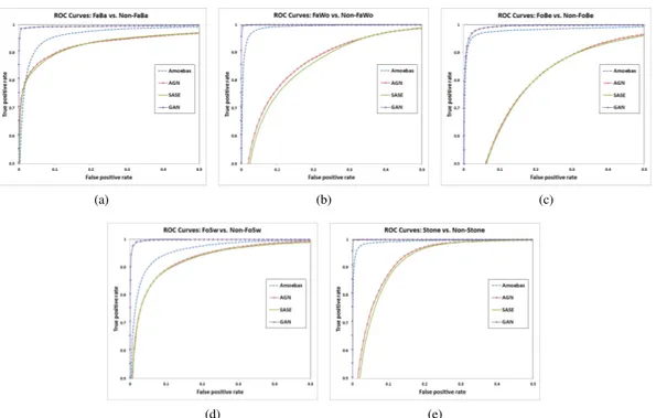
Some authors claim that the hit rate is not the most suitable measure to illustrate the performance of a classifier, and that a ROC analysis would be more convenient [17]. However, this is not a binary classification problem as, indeed, a five-way classifier has been used, so it is not straightforward to carry out such analysis. In this case, a ROC analysis of each ”binarized” problem (i.e. one class vs. the others) has been made, as it is done in [16]. The ROC space for each problem is presented in Fig. 3. Therefore, subfigure 3(a) display the FaWi versus non-FaWi (class 1 versus clases 2 to 5) binary ROCs achieved with the classifiers generated by each of the assessed descriptors. Similarly, the FaWo versus non-FaWo, FoBe versus non-FoBe, FoSw versus non-FoSw and Stone versus non-Stone comparisons are shown in subfigures 3(b), 3(c), 3(d), and 3(e), respectively. In addition, the areas under these curves (AUC) are shown in table III.

Regarding these results in table III, the classifiers generated using GAN-based descriptors achieve the best AUCs (ROC curves in these cases are, actually, close to ideal curves, as their AUC is close to 1). Although always below GANs, amoeba-based classifiers also achieve excellent performances (comparable to GANs in Stone and FaWo problems, as it is depicted in Fig. 3). The less successful classifiers are the ones based on AGNs and SASEs, depending on the problem. It is remarkable the difference in AUC between GANs and amoebas compared to its difference in accuracy. It actually shows that classifiers generated by amoeba-based descriptors are very successful when classifying a pixel as belonging or not to one class. However, when assigning them to one amongst other classes, GAN-based descriptors seem more efficient.

With respect to the computational complexity, the average computation time necessary to describe all pixels has been computed. The fastest method was the GAN-based one (70.47 seconds against 311.65 for the MA, 279.42 for the AGN and 601.35 for the SASE).

VI. CONCLUSION

In this paper a new pixel descriptor based on the General Adaptive Neighborhood (GAN) framework for gray-level im-ages has been presented. Concretely, each pixel is described by a concatenation of integral geometry and morphometrical functionals measured from GANs of different sizes and gray-level values of GAN-based adaptive erosions and dilations.

For the sake of comparison, other adaptive neighbor-hoods proposed in the literature have been used to compute this descriptor: Morphological Amoebas, Adaptive Geodesic

(a) (b) (c)

(d) (e)

Fig. 3. Top-left part of the ROC graphs for the classifiers generated with the data corresponding to the compared methods for each binary classification problem: FaBa vs. non-FaBa (a), FaWo vs. non-FaWo (b), FoBe vs. non-FoBe (c), FoSw vs. non-FoSw (d) and Stone vs. non-Stone (e).

Neighborhood and Salience Adaptive Structuring Elements. These four methods were compared using textures from five different classes extracted from the VisTex database.

The GAN-based descriptor achieved an overall accuracy of 97.25%, while amoebas, AGN or SASE ones achieved 91.13%, 75.04% and 68.18%, respectively.

In future work, the extension of this descriptor for color images will be addressed by using the generalization of GANs to color images [18]. In addition, this method may be a really good asset for image segmentation applications, or even for texture classification (e.g. using the histogram or other features from the maps of the texture). Therefore, its application to this kind of problems will be tackled.

ACKNOWLEDGMENT

This work has been supported by the project with reference ANR-12-EMMA-0046 from the French National Research Agency (ANR)

REFERENCES

[1] J. Debayle and J.-C. Pinoli, “General Adaptive Neighborhood Image Processing: Part I: Introduction and Theoretical Aspects,” Journal of Mathematical Imaging and Vision, vol. 25, no. 2, pp. 245–266, 2006. [2] J.-C. Pinoli and J. Debayle, “General adaptive neighborhood

mathe-matical morphology,” in Image Processing (ICIP), 2009 16th IEEE International Conference on, 2009, pp. 2249–2252.

[3] S. Rivollier, J. Debayle, and J. C. Pinoli, “Integral geometry and general adaptive neighborhood for multiscale image analysis,” International Journal of Signal and Image Processing, vol. 1, no. 3, pp. 141–150, 2010.

[4] S. Rivollier, J. Debayle, and J.-C. Pinoli, “Adaptive shape diagrams for multiscale morphometrical image analysis,” Journal of Mathematical Imaging and Vision, pp. 1–18, 2013, accepted paper.

[5] R. Lerallut, ´Etienne Decenci`ere, and F. Meyer, “Image filtering using morphological amoebas,” Image and Vision Computing, vol. 25, no. 4, pp. 395–404, 2007.

[6] J. Grazzini and P. Soille, “Edge-preserving smoothing using a similarity measure in adaptive geodesic neighbourhoods,” Pattern Recognition, vol. 42, no. 10, pp. 2306–2316, 2009.

[7] V. ´Curi´c, C. Luengo Hendriks, and G. Borgefors, “Salience adaptive structuring elements,” Selected Topics in Signal Processing, IEEE Journal of, vol. 6, no. 7, pp. 809–819, 2012.

[8] K. Michielsen and H. D. Raedt, “Integral-geometry morphological image analysis,” Physics Reports, vol. 347, no. 6, pp. 461 – 538, 2001. [9] K. Mecke and D. Stoyan, Eds., Statistical Physics and Spatial Statistics.

Springer-Verlag Berlin and Heidelberg, 2000.

[10] G. Matheron, Random Sets and Integral Geometry, J. W. . Sons, Ed. John Wiley & Sons, 1975.

[11] J. Serra, Image Analysis and Math. Morphology, A. Press, Ed. Aca-demic Press, 1982.

[12] S. R. Sternberg, “Grayscale morphology,” Comput. Vision Graph. Image Process., vol. 35, no. 3, pp. 333–355, 1986.

[13] P. L. Rosin and G. A. West, “Salience distance transforms,” Graphical Models and Image Processing, vol. 57, no. 6, pp. 483–521, 1995. [14] V. Gonz´alez-Castro, E. Alegre, O. Garc´ıa-Olalla, L. Fern´andez-Robles,

and M. Garc´ıa-Ord´as, “Adaptive pattern spectrum image description using euclidean and geodesic distance without training for texture classification,” Computer Vision, IET, vol. 6, no. 6, pp. 581–589, 2012. [15] G. Zhang, “Neural networks for classification: a survey,” Systems, Man, and Cybernetics, Part C: Applications and Reviews, IEEE Transactions on, vol. 30, no. 4, pp. 451–462, 2000.

[16] J. Arribas, V. Calhoun, and T. Adali, “Automatic bayesian classification of healthy controls, bipolar disorder, and schizophrenia using intrinsic connectivity maps from fmri data,” Biomedical Engineering, IEEE Transactions on, vol. 57, no. 12, pp. 2850–2860, 2010.

[17] T. Fawcett, “An introduction to ROC analysis,” Pattern Recognition Letters, vol. 27, no. 8, pp. 861–874, 2006.

[18] J. Debayle and J. C. Pinoli, Advances in Low-Level Color Image Pro-cessing, ser. Lecture Notes in Computational Vision and Biomechanics. Springer, 2014, vol. 11, ch. Spatially Adaptive Color Image Processing.