Coupled methods of nonlinear estimation and control applicable to terrain-aided navigation

(1)

HAL Id: tel-02396908

https://pastel.archives-ouvertes.fr/tel-02396908

Submitted on 6 Dec 2019

HAL is a multi-disciplinary open access

archive for the deposit and dissemination of sci-entific research documents, whether they are pub-lished or not. The documents may come from teaching and research institutions in France or abroad, or from public or private research centers.

L’archive ouverte pluridisciplinaire HAL, est destinée au dépôt et à la diffusion de documents scientifiques de niveau recherche, publiés ou non, émanant des établissements d’enseignement et de recherche français ou étrangers, des laboratoires publics ou privés.

Coupled methods of nonlinear estimation and control

applicable to terrain-aided navigation

Emilien Flayac

To cite this version:

Emilien Flayac. Coupled methods of nonlinear estimation and control applicable to terrain-aided navigation. Optimization and Control [math.OC]. Université Paris-Saclay, 2019. English. �NNT : 2019SACLY014�. �tel-02396908�

(2)

THÈSE DE DOCTORAT

de

l’Université Paris-Saclay

École doctorale de mathématiques Hadamard (EDMH, ED 574) Établissement d’inscription : École nationale supérieure de techniques avancées Établissement d’accueil : Office national d’études et de recherches aérospatiales Laboratoire d’accueil : Unité de mathématiques appliquées, ENSTA-CNRS-INRIA

Spécialité de doctorat : Mathématiques appliquées

Emilien FLAYAC

Coupled methods of nonlinear control and estimation applicable to

Terrain-Aided Navigation

Jury de soutenance :

Daniel Kuhn (Ecole Polytechnique Fédérale de Lausanne)Rapporteur

Silvère Bonnabel (MINES Paristech)Rapporteur

François Le Gland (INRIA Rennes)Président du Jury

Tarek Hamel (Université Nice Sophia Antipolis)Examinateur

Pierre Carpentier (ENSTA Paris)Examinateur

Frédéric Jean (ENSTA Paris)Directeur de Thèse

Karim Dahia (ONERA)Encadrant

(3)

(4)

Acknowledgements

Je souhaiterais remercier toutes les personnes qui m’ont permis de réaliser cette thèse dans de très bonnes conditions, à commencer par Silvère Bonnabel et Daniel Kuhn qui ont accepté d’être mes rapporteur de thèse. Je remercie aussi Tarek Hamel, François Le Gland et Pierre Carpentier de bien avoir voulu être membres de mon jury de thèse.

Je voudrais exprimer ma sincère gratitude envers mes deux encadrants de thèse de l’ONERA, Bruno Hérissé et Karim Dahia qui m’ont soutenu et supporté pendant trois ans, ce qui ne fut pas de tout repos à mon avis. Cette gratitude s’étend bien sûr à mon directeur de thèse, Frédéric Jean, qui a toujours su m’apporter ses conseils et ses critiques aux bons moments depuis qu’il a commencé à suivre mon parcours.

Je me dois de mentionner mes amis de promotion de l’ENSTA que je ne cesserai d’épargner et qui en feront toujours de même, à juste titre. En particulier, bien qu’il soit docteur en Automatique, je remercie Benoît Bonnet pour son oreille scientifique et humaine attentive et toujours pertinente. J’ai une pensée impériale et impérieuse pour Florian Enaud, grand stratège du hasard de notre amitié. J’aime penser que Thomas Bourguenolle a rejoint ce monde pour compenser mon manque de "skill" et moi son manque de "fail". Je dois aussi parler d’Hadrien Godard alias "Banach" qui, faute d’avoir les compétences d’un mathématicien, en a le surnom. Je finirai cette liste par Rémi Lucas, passionné par ce qui n’est pas passionnant et par Rémi Feuillet adorateur des maillages, de René Coty et des maillages de René Coty.

Parmi les doctorants de l’ONERA que j’ai cotoyés pendant trois ans, qui m’ont aidé et que, plus rarement, j’ai aidé, je remercie Vincent, Iréna, Romain, Nicolas, i.e. les très vieux, puis Nathan, Léon, Sergio, Julien et Camille la grande, i.e. les vieux comme moi, et enfin les stagiaires ou assimilés, comme Ali, Esteban, Etienne, Rodolphe, Guillaume, Camille la jeune, Jean-Lynce, Baptiste, Antonella, Thomas (mon stagiaire) et bien d’autres dont j’ai oublié le nom (Enzo par exemple). Je voudrais aussi remercier tous les membres de l’unité NGPA, pour leur bonne humeur, leur sympathie et leurs afterworks mé-morables. Je vais m’attarder sur Ioannis Sarras, car il m’a fourni beaucoup de conseils pratiques sur le déroulement d’une thèse et beaucoup d’aide scientifique sur des sujets que je ne maitrisais pas du tout, en arrivant à l’ONERA.

Finalement, je remercie les membres de ma famille ou ceux considérés comme tel, en commençant par Kester James Bradbury dont l’impertinence molle et la folie rêveuse me complètent depuis dix ans. J’ai une pensée particulière pour ma mamie, Monique, et son soutien indéfectible et pour mon oncle, Alain et ma cousine, Emma qui m’enjaillent au détour de soirées parisiennes par leur poésie du quotidien. Que dire de ma soeur, Justine et de mon beau-frère Nicolas à part qu’ils m’ont beaucoup invité chez eux et que je suis peu venu.

Mon dernier mot sera dedié à mes parents Serge et Isabelle à qui je dois d’être qui je suis et ce que je suis dans ce monde à savoir un don ou une malédiction.

(5)

(6)

Résumé

Dans cette thèse, nous étudions les problèmes de contrôle et d’estimation non linéaire couplés avec ap-plication à la navigation par corrélation de terrain (TAN en anglais). L’objectif est de guider et d’estimer la position 3D d’un drone survolant une zone connue. La principale difficulté de cette application est la nature de l’information disponible sur le système. En effet, on suppose que les seules données disponibles sont la vitesse du système, une mesure de hauteur/sol et une carte de la zone survolée. Comme la carte est généralement créée avec des données empiriques, cela pose un problème d’estimation très complexe en soi qui a été étudié de manière approfondie depuis les années 50.

Habituellement, les problèmes d’estimation et de contrôle sont résolus séparément en invoquant le classique principe de séparation qui stipule que de bonnes performances peuvent être obtenues en com-binant un contrôleur avec information parfaite et un estimateur conçu indépendamment.

Cependant, le principe de séparation n’est applicable que pour des classes de systèmes très partic-ulières, dont les systèmes linéaires. Ainsi, pour un système non linéaire général, le contrôle et l’estimation doivent être gérés conjointement. La TAN est un bon exemple d’application non linéaire où le principe de séparation ne peut pas être appliqué. En réalité, la qualité des observations dépend du contrôle et plus précisément de la zone survolée par le drone. En conséquence, Les sujets suivant ont été étudiés

• La conception d’observateurs non linéaires et contrôle en retour de sortie pour la TAN avec des cartes analytiques au sol dans un cadre temporel continu.

• Le problème couplé du filtrage optimal non linéaire et du contrôle optimal stochastique en temps discret avec des informations imparfaites.

• La conception de schémas de commande prédictive duale explicite couplés à un filtre particualrie et leur implémentation numérique vers une application non linéaire (y compris la TAN).

Concernant le premier sujet, la technique d’immersion et d’invariance a été utilisé pour concevoir des observateurs non linéaires capables de reconstruire la position 3D du drone dans plusieurs cas de cartes au sol (quadratiques, cubiques, gaussiennes). Il a été démontré que, sous condition de persistance d’excitation sur la vitesse horizontale, l’erreur d’estimation converge vers zéro. Le problème de contôle en retour de sortie a également été étudié en utilisant le concept de δ -persistance. Concernant le deuxième sujet, une reformulation des problèmes de filtrage optimal non linéaire et de contrôle optimal stochastique en temps discret avec information imparfaite en un seul problème d’optimisation a été proposée. Cela per-met de justifier l’utilisation de deux étapes dans la résolution du problème sous des hypothèses naturelles sur la fonction de coût. La première étape consiste à résoudre un problème classique d’estimation opti-male. La quasi-optimalité de la moyenne empirique d’un filtre particulaire modifié par rapport à l’erreur quadratique moyenne a été montrée dans cette thèse. Cela justifie l’utilisation du filtrage particulaire. La deuxième étape consiste à résoudre un problème de contrôle optimal modifié avec un nouveau terme issu d’une estimation optimale. Ceci établit une connexion avec le contrôle dual explicite dans lequel un nou-veau terme représentant une mesure d’information est ajouté empiriquement au coût. En réalité, ce terme

(7)

vi

empirique peut être vu comme une approximation du terme issu de l’estimation optimale. En ce qui con-cerne le troisième sujet, les filtres de Kalman sont répandus dans l’estimation d’états mais connus pour être inefficaces pour la TAN contrairement aux filtres particulaires. En conséquence, au cours de cette thèse, deux contrôleurs prédictifs stochastiques explicites duauxen retour de sortie pour des systèmes non linéaire généraux, couplés à un filtre particulaire, ont été conçus et appliqués à la TAN. Les deux schémas sont basés sur l’integrated experiment design, mais l’un contient une pénalisation de l’objectif de guidage dans le coût et l’autre utilise une contrainte de Lyapunov. Les problèmes d’optimisation résultants sont résolus grâce à une méthode d’approximation de Monte Carlo et les deux contrôleurs ont montré de bons résultats en simulation.

(8)

Introduction

Problems of control and state estimation of dynamical systems with imperfect information are widespread, for instance, in chemical engineering [Kumar and Ahmad, 2012], in electrical and mechanical engineer-ing [Bolton, 2003], in mathematical finance [Mamon and Elliott, 2007] and in aerospace engineering [Eren et al., 2017]. In this work, we study nonlinear coupled control and estimation problems in order to solve a challenging application that is Terrain-Aided Navigation (TAN). The objective is to guide and estimate the 3D position of a drone flying over a known area. The main difficulty of this application is the nature of the available information on the system. Indeed, it is assumed that the only available data are the speed of the system, a measurement of the height from the ground and a map of the area flied over. As the map is generally created with empirical data, this leads to a very complex estimation prob-lem in itself which has been thoroughly studied since the 50’s ([Dahia, 2005], [Melo and Matos, 2017], [Sabatino et al., 2003]). Thus, adding guiding to the problem makes it even harder and lacks of treatment in the literature.

Usually, estimation and control problems are solved separately invoking the classical separation prin-ciple which states that good performance can be achieved by combining a controller with perfect infor-mation on the state and an independently devised estimator. See [Hespanha, 2009] and [Bertsekas, 1995] for examples in different frameworks.

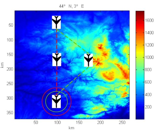
However, the separation principle is known to hold true only for very particular classes of systems including linear systems. Thus, for a general nonlinear system, control and estimation must be handled jointly. TAN is a good example of nonlinear application where the separation principle cannot be applied. Actually, the quality of the observations depends on the control and more precisely on the area that is flied over by the drone. Figure1.1depicts two typical trajectories of a drone in TAN. The ellipses represent the uncertainty on the final state. The red trajectory corresponds to flight over a flat area with constant altitude. In this case, one measurement of height matches a whole horizontal area and the estimation error on the horizontal position is of the same order of magnitude as the size of the area which can be very large. On the contrary, if the drone flies over a rough terrain, which corresponds to the green trajectory, then one measurement of height corresponds to a smaller area on the ground. The estimation error is then reduced, as shown in Figure1.1where the green ellipse is smaller than the red one.

The main objective of the thesis is to tackle this problem and to design coupled control and estimation methods for nonlinear dynamical systems applicable to terrain-aided navigation.

In Part I, we put ourselves in a simplified framework of TAN to understand how the control can influence observability and how to build observers and control laws accordingly. Firstly, in Chapter2,

(11)

2 CHAPTER 1. INTRODUCTION

Figure 1.1: Example of trajectories of a UAV flying over a real terrain

we assume that the dynamics of the drone is a deterministic double integrator in continuous time. We represent the state of the system with the 3D position, the 3D speed and with the control being the 3D acceleration. We also assume that the altitude of the ground is represented by a map hM from R2to R which is a polynomial, a Gaussian, a sum of Gaussians or a Fourier serie. This modelling simplifications allow us to get insight on which trajectory the drone must follow to be able to reconstruct its position. It is done by computing the classical conditions for local weak observability [Besançon, 2007]. Actually, it emerges that observability is guaranteed if the horizontal speed and acceleration are not colinear.

This condition is related to persistence of excitation (PE) of the horizontal speed. In adaptive control, PE describes the fact that a vector signal must explore sufficiently many linearly independent directions in the state space. This allows one to excite the system and make the estimation of some unknown parameters possible (see [Narendra and Annaswamy, 2012]).

Following this concept in Chapter3, we propose new observers for TAN based on two variants of the Immersion and Invariance (I&I) technique [Astolfi et al., 2008] and a controller designed accord-ingly. Observer design by I&I consists in defining a nonlinear estimation error in the augmented space (state/observer) so that the manifold where the error vanishes is invariant and attractive. Our first

(12)

ap-3

proach is to directly handle the nonlinearity of the map in the design of the nonlinear estimation error. This technique has been successfully applied to the case of a polynomial map of degree 2 and a Gaussian map with an additional measurement of the absolute altitude. In [Martin and Sarras, 2018], a similar technique is used to show global convergence of a state observer for a particular nonlinear system. How-ever, some maps are too complex to be tackled directly. Our second approach is then to immerse the original system into a higher dimensional one for which observer design is easy. Eventually, one has to make sure that the higher dimensional observer can be used to estimate the original system. This method has been applied to the case of a cubic map and partially to the case of a trigonometric map.

In the direct approach, the resulting estimation error equation is very well-known in adaptive control. Moreover, global convergence of the estimation error to zero is proven under a condition of persistence of excitation on the horizontal speed. Intuitively, it states that the system must avoid to go in straight line. In the indirect approach, a PE condition is still required but it is harder to interpret. PE has been widely studied but it is still not obvious how to incorporate it in an output-feedback loop. Besides, continuous time almost sure stochastic PE conditions have not been extensively studied.

That is why, afterwards, we focus on finding interesting sufficient conditions for the convergence of the previous observers, in terms of output-feedback control and stochastic excitation.

It is rather simple to design a control law that ensures a PE condition on the speed. However, persistent signals generally do not converge, think of sinusoidal signals for example. It means that, if one tries to achieve output-feedback asymptotic stability, the speed cannot be persistent as classically defined. Moreover, a stabilising controller is generally not persistent enough to ensure the convergence of the estimation error to zero. Accordingly, an idea is to enforce the speed to verify a condition of δ-persistence inspired from [Loría et al., 1999] and [Loría et al., 2002] which allows the whole system to converge. More precisely, the speed is persistent with a time varying level of excitation. The latter is usually made to decrease as some norm of the state of the system. This allow the true state of the system to converge to an equilibrium point while ensuring that the estimation error goes to zero.

However, to apply existing results in [Loría et al., 2002], the level of excitation should be an increas-ing and zero at zero function of the norm the estimation error. Although, the latter is unknown at all time so it cannot be used in the design of the controller. Consequently, we choose to make the level of excita-tion of the speed diminish as the estimated trajectory converges to the equilibrium. The main drawback of the method is that, if the estimated trajectory converges too quickly, the level of excitation reaches zero before the estimation error become small. However, we show that if the estimated trajectory converges sufficiently slowly to the equilibrium then the whole system verifies the property of semi-global practical stability.

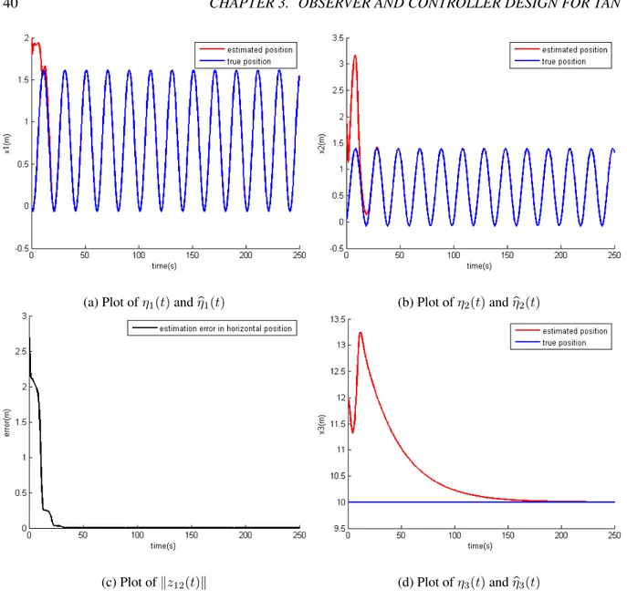
The observer-controller performances are validated by numerical simulations in above cited cases. In practice, the controller is composed of a stabilising term plus a term which is δ-persistent with respect to the speed and the state of the observer. The excitation can be introduced by any classical PE signal like si-nusoidal ones. Although, in simulations, stochastic signals may also be sufficient. In [Loría et al., 2002], a Gaussian white noise is used. We give a new example of 2D rectangular processes that are almost surely PE with a random level of excitation.

To sum up PartI, the observability properties of TAN with several types of analytical ground maps are first studied in Chapter2. Then, Chapter 3is dedicated to the design of nonlinear observers and control laws with a focus on the condition of persistence of excitation of the horizontal speed. Restricting ourselves to analytical ground maps gives us an intuition and some avenues on how to deal with TAN for real maps. Still, the previous framework does not provide good results for more complicated maps like a sum of Gaussians even if the observability conditions are similar. Actually, the additional nonlinearity in these cases makes the problem of finding a globally convergent observer too difficult.

(13)

Therefore, in PartII, we decide to tackle the problem of estimation and control with terrain-aided measurement for a real ground map in a discrete time stochastic framework. Concretely, our first mo-tivation is to be able to use stochastic filters like particle filters to estimate the state of the drone. Our second motivation is to use techniques from stochastic control with imperfect information, such as dual stochastic Model Predictive Control, to couple the design of the estimator and of the controller.

To do so, we consider a general non-linear Markov chain to represent the state of the system and a nonlinear observation equation to represent the noisy partial measurements. In this framework, as one considers general non vanishing stochastic perturbation in a nonlinear system, it is impossible to get exact output-feedback convergence of the state of the system or exact convergence of an estimator to the true state. That is why, we decide to choose an optimisation-based solution to deal with estimation and control.

In Chapter4, we recall the fundamentals of stochastic control and filtering. On one hand, there is the state estimation problem. In this framework, it corresponds to finding an estimator of the state as a func-tion of the available informafunc-tion that minimised some estimafunc-tion error. Customarily, one tries to minimise the mean square error between the state and the estimator. In this case, the best estimator is the conditional expectation of the state with respect to all the available information. Additionally, if the system is linear Gaussian then the Kalman filter gives the optimal solution in closed form [Anderson and Moore, 1979]. Although, for a general nonlinear non-Gaussian system, there is a closed form neither for the conditional expectation nor for the conditional distribution (also called the filtering distribution). However, the latter verifies a recursive equation, the so-called filtering equation, which is itself intractable. Consequently, in practice, only approximations of the filtering equation are computed. Among the popular approxima-tions are Extended Kalman filters, Unscented Kalman filters, Ensemble Kalman filters and particle filters. Recently, particle filters have demonstrated their performance in terrain-aided navigation [Dahia, 2005], [Murangira, 2014]. The principal reason is that particle filters (PF) can deal with nonlinear dynamics or observation equation and with multimodal uncertainties which both appears in TAN. That is why, we focus on PF in the following.

On the other hand, in the stochastic control framework, one does not look for control values but rather for control policies that are measurable functions that map the available information to a control value. An important property of the control when only partial information is available is that the controller must look for more information to ensure a good estimation and a better control in the end. In other words, for a general system, the controller may degrade the available information and prevent one from building good estimators. This property, referred as the dual effect property, was first brought to light by Feldbaum in his seminal work [Feldbaum, 1960]. It also means that the separation principle does not apply in general. In [Bar-Shalom and Tse, 1974], a classification of control policies according to their level of information use and probing is presented. It goes from open loop controls, where one looks for controls values depending only on the initial information, to closed loop controls, where the current information is used and the future one is predicted in some way. In the case of stochastic optimal control with imperfect information as described in the survey paper [Mesbah, 2017], one can see from the Dynamic Programming (DP) principle [Bertsekas, 1995] that optimal controls have the dual effect properties. In this case, it is called implicit dual effect because it is only due to the optimality of the controller without external excitation. However, as these problems are intractable in practice, suboptimal output-feedback control laws are computed instead, with the idea to keep the dual effect property. They are called dual controllers. There exist two kinds of dual controllers: implicit and explicit ones. The idea behind implicit dual controllers is to keep the natural implicit dual effect coming from optimal controls by approximating the DP equation. We do not consider implicit dual controllers in this work as they are very difficult to combine with PF and computationally costly. Instead, we consider explicit

(14)

5

dual controllers which are derived by solving a related open loop control problem where a measure of information is added to the cost. This new cost allows the controller to recover the dual effect lost by doing an open loop approximation. The main drawback of these controllers is that the measure of information is generally empirical and hard to make theoretically grounded.

Therefore, our first contribution, gathered in Chapter5, consists in the definition a new infinite hori-zon multistage stochastic optimisation problem that gathers a stochastic optimal control problem with imperfect information and an optimal estimation problem. This problem can be recast as a classical infinite-time stochastic optimal control problem with imperfect information by considering an augmented control. The augmented controls are composed of an estimation policy and of the original control policy. By applying the DP principle to this problem and, under natural assumptions on the cost function, one can justify the use of two steps in the resolution of the problem:

• The first step is to solve a classical optimal estimation problem. From a more theoretical perspec-tive, one would like to know if the Mean Square Error (MSE) associated with the empirical mean of a PF converges to the optimal MSE, the one associated with the true conditional expectation. There exist many results of convergence of PF to the true filtering distribution as the number of particles goes to infinity. In [Crisan and Doucet, 2002], and [Arnaud Doucet et al., 2001] several convergence results and error bounds are surveyed. The most classical error bounds involve inte-grals of bounded continuous functions of the PF and the filtering distribution. These results do not allow us to conclude as the mean is the integral of the identity which is unbounded. Surprisingly, very few results concerning integrals of unbounded functions exist. Nevertheless, using the results of [Hu et al., 2011], we provide an error bound between the MSE of the PF and the optimal one, for a specific PF algorithm and a rather large class of models that contains TAN. Thus, the modified PF solves approximately the optimal estimation problem for a square estimation error.

• Once optimal or near optimal estimation is achieved, we show that, to solve our new optimisation problem, the last step is to solve a stochastic optimal control problem with imperfect information where the cost function is composed of two terms that are contradictory in general. The first one is the estimation error associated to the optimal estimator seen as a function of the state and the available information. The second one is a classical cost function depending on the control and on the state which can be, for instance, an economic cost, a penalisation of some guiding goal or a combination of the two. Consequently, our claim is that classical explicit dual control problems are approximations of the former optimal control problem. The estimation-based term which is generally unknown is replaced by a related one usually independent of the observations such as the Fisher Information Matrix.

One of the most common method to solve approximately infinite time stochastic optimal control problems is Stochastic Model Predictive Control (SMPC). It consists first in solving a finite horizon problem at the current. Then, one keeps and applies only the first optimal control to the true system. Finally, these computations are repeated starting from the new current state in a receding horizon way. In the case of partial information, the current state is usually replaced by the current estimation. A lot work has been done using Kalman-like filters [Hovd and Bitmead, 2004], [Subramanian et al., 2015], [Heitsch and Römisch, 2009], [Heirung et al., 2015]. Although few MPC methods uses PF in the litera-ture (see [Sehr and Bitmead, 2016]).

Following the previous algorithm scheme, our second main contribution, gathered in Chapter6, con-sists in the design of two dual output-feedback SMPC methods which includes a particle filter for state estimation. The first one consists in coupling a particle filter with the resolution by a Monte Carlo method

(15)

of an explicit dual stochastic optimal control problem. The initial condition of each Monte Carlo trajec-tory is chosen to be a particle from the particle filter. This allows the control to be aware of the multimodal uncertainty on the state which is more difficult or even impossible with a Kalman-like filter. This has been used in [Sehr and Bitmead, 2016] but not in the framework of dual control. The main drawback of this method is that the cost function of the optimisation problem combines a stabilising term and an information probing term. This creates a trade-off between going toward the guiding goal and looking for more information. Indeed, if too much importance is given to the information term then probing will be efficient but the system may get stuck far from the target. Conversely, if too much importance is given to the stabilising term then the probing effect will not be sufficient and output-feedback performance may be poor. It is difficult to know which case will occur beforehand. As a consequence, we propose another dual MPC where the guiding objective is dealt with by a Lyapunov constraint coming from the theory of Markov chain stability. The main consequence is that there is no more trade-off between guiding and in-formation probing inside the cost. We prioritise the guiding goal and we only look for stabilising controls that maximise the expected information.

Finally, these two algorithms are applied to TAN with a real ground map. The main challenge is to solve the stochastic optimal control problem numerically. To do so, we consider a Monte Carlo ap-proximation and solve it with a nonlinear programming solver. Besides, the real ground map is usually obtained from discrete data. Thus, one has to interpolate the map during the resolution.

To sum up PartII, the basics of stochastic control and filtering are first described in Chapter4. Sec-ondly, the modelling of state estimation and stochastic optimal control for a general nonlinear system gathered in one global stochastic optimisation problem is presented in Chapter5. Finally, in Chapter6, two explicit dual output-feedback stochastic MPC schemes based on particle filtering are proposed and tested on TAN with a real ground map.

(16)

Part I

Terrain-Aided Navigation with analytical

ground maps

(17)

(18)

Chapter 2

Terrain models and observability

conditions

In whole PartI, we consider the problem of Terrain-Aided Navigation in a simplified deterministic con-tinuous time framework. The ground profile is assumed to be a simple known functions or combinations of simple ones. The goal of this part is twofold. First, one would like to design observers and controllers for as many different models of TAN as possible. Secondly, one is looking for some insight on how to solve the problem of TAN with a complicated real maps. In Chapter2, we define the several models of maps and study the intrinsic observability properties of the resulting controlled system. One is willing to identify the influence of the control on the observability of these systems.

2.1 General nonlinear observability conditions

2.1.1 General nonlinear controlled system

First, consider the following general nonlinear controlled dynamical system: 9

x(t) = f (x(t), u(t)),

y(t) = h(x(t), u(t)), (2.1)

where ∀t ≥ 0:

• x(t) ∈ Rn_{is the state of the system.}

• x(0) = x0where x0∈ Rnis an initial condition. • y(t) ∈ Rp_{is the output of the system.}

• u(t) ∈ Rm_{is the input of the system. We denote by U, the set of possible input u(·).}

• f : Rn_{× R}m _{−→ R}n_{represents the dynamics of the system and is assumed to beC}∞_{in x and u.} • h : Rn_{× R}m_{−→ R}p_{is the observation function that links the output y(t) to the state x(t). In the}

following, we also assume that h is C∞_.

This model will be used in the following to present some general concepts in nonlinear observability theory and nonlinear observer design.

(19)

10 CHAPTER 2. TERRAIN MODELS AND OBSERVABILITY CONDITIONS

2.1.2 General definitions of observability

We consider a general nonlinear model of the form (2.1). We fix an input u(·) and an initial condition x0. we define x(t; x0, u(·)) as the solution of equation (2.1) starting from x0 with input u(·). As the model is nonlinear, classical Kalman rank condition [Hespanha, 2009] does not apply. Moreover, the observability properties depend on the input.

2.1.2.1 Local weak observability

We would like to check if one is able to discriminate x0from all other initial conditions using the output y(·)and the control u(·). This is a problem of observability.

In the following, we recall several classical notions of nonlinear observability borrowed and adapted from those in [Besançon, 2007]. It is important to notice that, as the input is fixed, we study the observ-ability of an uncontrolled system parametrised by u(·). First we consider the definition of distinguishable states.

Definition 2.1. A pair (x0, x00) ∈ (Rn)2is distinguishable with input u(·) if, ∃t ≥ 0 such that: h(x(t; x0, u(·)), u(·)) 6= h(x(t; x00, u(·), u(·)).

A state x is said to be distinguishable from x0 with input u(·) if the pair (x, x0)is distinguishable with

input u(·).

It is different from classical distinguishability defined in [Besançon, 2007]. Usually, one looks at ev-ery possible input and shows that there exists one that is able to separate two different initial conditions. Distinguishability from an particular initial condition with respect to some particular input is more con-cerned with checking that a proposal input allows to discriminate this initial condition from other ones. From this version of distinguishability, we define local weak observability at x0with input u(·).

Definition 2.2. The system (2.1) is said to be locally weakly observable at x0 with input u(·) if there

exists a neighbourhood of x0, U, such that ∀x00∈ U, ∃t ≥ 0 such that: h(x(t; x0, u(·)), u(·)) 6= h(x(t; x00, u(·), u(·)),

x(t; x0₀, u(·)) ∈ U.

This notion means that one can distinguish all states near x0 while staying near x0 using the input u(·). Therefore, this kind of property has a practical interest but is hard to check this form. That is why we define the notion of observability space. As we are concerned with local properties for the moment, we look for control values that locally allows observability. Thus we consider in the following definition that u(·) ≡ u0with u0∈ Rm.

Definition 2.3. The observability space with constant input u0, denoted by Ou0(h), is the smallest real

vector space of C∞_{functions from R}n_{to R that contains the components of h(·, u}

0)and is stable under

the Lie derivative Lu0 which is defined by:

L_u₀φ = dφf (x, u0)

The notion of observation space allows to write a sufficient condition of local weak observability based on a rank condition.

(20)

2.2. OBSERVABILITY PROPERTIES IN TERRAIN-AIDED NAVIGATION 11

Definition 2.4. The system (2.1) is said to verify the observability rank condition at x0with input u0if: dim(dOu0(h)|x0) = n

where dOu0(h)|x0 is the set of dφ(x0)with φ ∈ Ou0(h)

Proposition 2.1. If the system (2.1) satisfy the observability rank condition at x0 with input u0, then it

is locally weakly observable at x0 with input u0.

Proof. The proof can be found for a more general case in [Hermann and Krener, 1977]. The idea is that the rank condition allows one to construct a local diffeomorphism around x0with functions from Ou0(h).

As these functions can be "observed", the result follows.

2.1.2.2 Universal and persistent inputs

Conditions of local weak observability from the last section give insight on how a constant control must be chosen depending on the initial state x0. We are now interested in finding conditions on the input u(·)to ensure that observability is preserved along the trajectory. This leads to the definition of universal inputs.

Definition 2.5. An input u(·) is an universal input on [0, t] if for any x0 6= x00, there exists τ ∈ [0, t] such

that h(x(τ; x0, u(·)), u(·)) 6= h(x(τ ; x00, u(·), u(·)).

From Definition2.5, one can derive an equivalent integral property:

Proposition 2.2. An input u(·) is universal on on [0, t] if and only if ∀x06= x00: Z t

0

kh(x(τ ; x₀, u(·)), u(·)) − h(x(τ ; x0₀, u(·)), u(·))k2dτ > 0.

Universal inputs are inputs that never destroy the observability of the system. A related property is the property of regular persistence of the input.

Definition 2.6. A input u(·) is said to be regularly persistent if ∃t0≥ 0, T > 0and there exists κ : R −→ R increasing with κ(0) = 0 such that, ∀t ≥ t0, ∀x 6= x0:

Z t+T t

kh(x(τ ; x, u(·)), u(·)) − h(x(τ ; x0, u(·)), u(·))k2dτ ≥ κ(kx − x0k).

Obviously, from Proposition2.2, a regularly persistent input is an universal input. Informally, a reg-ularly persistent input excites the system consistently to ensure observability on a receding time horizon. It happens to be a useful property to force the convergence of some observers.

2.2 Observability properties in Terrain-Aided Navigation

The objective of this section is to check the observability rank condition in Terrain-Aided Navigation. To do so, we first define several models of ground maps in closed form and then apply the theory from Section2.1.1.

(21)

Figure 2.1: Example of a UAV localized by Terrain-Aided Navigation

2.2.1 Dynamical models for Terrain-Aided Navigation (TAN) with closed-form ground maps

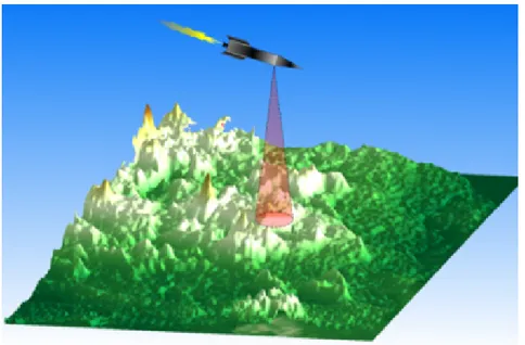
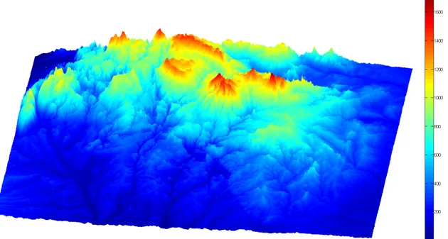
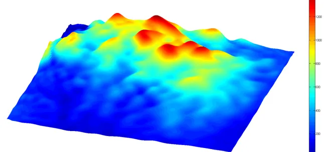
We consider the scenario of a drone evolving in a 3D space without direct measurements of its 3D po-sition. This scenario can occur after a GPS failure or simply because GPS devices are not used as they are easy to jam. It is assumed instead that the drone is equipped with a radar-altimeter. A radar-altimeter gives a measurement of the vertical distance between the drone and the ground. It is also assumed that the terrain flied over by the drone is known. The issue of the following is to determine if these two pieces of information are sufficient to reconstruct the horizontal and the vertical position of the drone. This problem is called Terrain-Aided Navigation and is represented in Figure 2.1. Figure2.2represents the test map that has been used throughout the thesis.

For the sake of simplicity, the drone is represented by a point in 3 dimensions and we suppose that either its 3D speed or its 3D acceleration is controlled. In any case, the inertial speed i.e. the speed in the inertial frame is supposed to be known. It is a substantial simplification as in many applications the inertial speed is not measured but the speed in the body frame is. Pose estimation is then generally needed to reconstruct the inertial speed. However, one can imagine that an external estimation loop is run such that the inertial speed is reconstructed precisely. Occasionally, we will assume that an addi-tional measurement of altitude is available mainly to simplify the design of some observers. It is not a restrictive assumption as baro-altimeters are very common in aircrafts. We make the previous sim-plifying assumptions because we want to focus on the main difficulty of the problem of TAN which is the nature of the available information on the position. Actually, the available information depends on the nature of the area that is flied over by the drone and consequently on the input. For example, let us assume that the drone flies over an ambiguous area, like a flat or a periodic one, with constant altitude then one measurement of height matches a whole horizontal area. The resulting estimation error on the horizontal position is of the order of magnitude of the size of the area which can be very large. On the contrary, if the drone flies over a rough terrain, then one measurement of height corresponds to a smaller

(22)

Figure 2.2: Example of a real terrain

area on the ground and the estimation error is reduced. Intuitively, the more perturbed the ground flied over is, the more information it contains. The idea of the following is to verify this intuition by studying the dynamical model of the drone with different types of maps.

Consequently, in the sequel, the dynamics of the drone is either a simple or a double integrator in 3D with control on the speed or on the acceleration.:

9 X = V, (2.2) or 9 X = V, 9 V = U, (2.3) where

• X = (x1, x2, x3) is the 3D position with (x1, x2) being the horizontal 2D position and x3 the altitude of the drone,

• V = (v1, v2, v3)is the 3D speed with (v1, v2)being the 2D horizontal speed and v3 the vertical speed. V is the input in the system (2.2),

• U = (u1, u2, u3)is the 3D acceleration with (u1, u2)being the 2D horizontal acceleration and u3 the vertical acceleration. U is the input in the system (2.3).

In the case where the inertial speed of the drone and its height with respect to the ground are measured, the observation equation reads:

(23)

14 CHAPTER 2. TERRAIN MODELS AND OBSERVABILITY CONDITIONS with h(X, V ) =„x3− hM(x1, x2) V  . If the altitude is also measured, the observation equation is written as follow:

y = halt(X, V ), (2.5) with halt(X, V ) = » – hM(x1, x2) x3 V fi fl,

where hM : R2 −→ R represents the profile of the ground. In equation (2.5), it is supposed that hM is measured because measuring x3and x3− hM is equivalent to measuring x3and hM.

In partI, we consider maps hM that can be written under closed form. In the sequel, we study in detail maps that have the following forms.

• A polynomial function of degree 2:

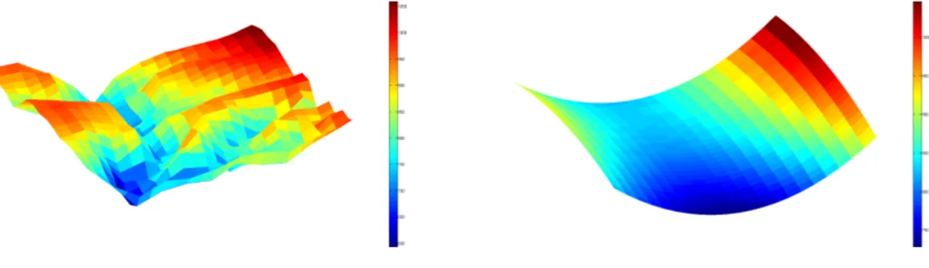
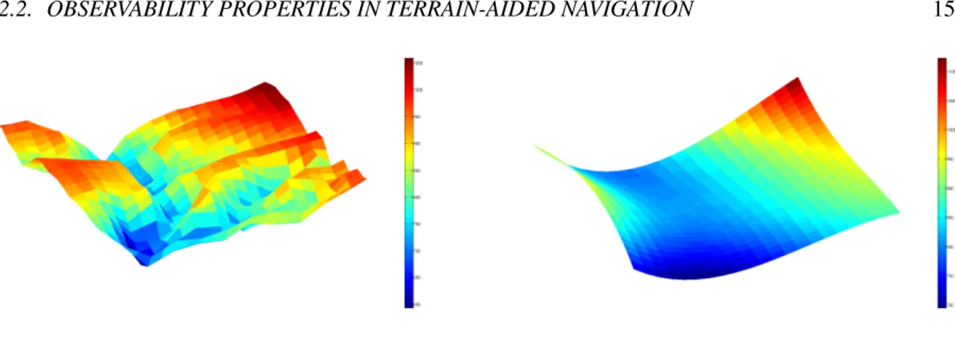
hM(x1, x2) = a20x21+ a11x1x2+ a02x22+ a10x1+ a01x2+ a00, (2.6) with (a20, a11, a02, a10, a01, a00) ∈ R6. Figure2.3represents a portion of the map presented in Figure2.2and its least-square polynomial approximation of order 2. It is a typical example of the possible uses of quadratic maps in TAN.

Figure 2.3: Representation of a part of the real map and its quadratic approximation

• A polynomial function of degree 3:

hM(x1, x2) = a30x31+ a21x12x2+ a12x1x22+ a03x32 (2.7) + a20x21+ a11x1x2+ a02x22+ a10x1+ a01x2+ a00,

with (a30, a21, a12, a03, a20, a11, a02, a10, a01, a00) ∈ R10. As in the quadratic case, Figure 2.4 represent a cubic approximation of the real map. For the sake of clarity, the approximations in Figure 2.3 and2.4 are done on a large area which make them rough. Indeed, in practice, one would need much more precise approximations.

(24)

Figure 2.4: Representation of a part of the real map and its cubic approximation

• A Gaussian function: hM(x1, x2) = H0exp ˆ −1 2“x1− x 0 1 x2− x02‰ R „x1− x01 x2− x02 ˙ , (2.8)

where H0 _{> 0}_{is the height of the Gaussian, X}0 _{= (x}0 1, x02)

T

∈ R2_{is the center of the Gaussian} and R is a symmetric positive definite 2 × 2 matrix that represents the width and the orientation of the Gaussian.

• A finite sum of Gaussian functions: hi_M(x1, x2) = Hiexp ˆ −1 2“x1− x i 1 x2− xi2‰ Ri „x1− xi2 x2− xi2 ˙ , hM = ng X i=1 hi_M, (2.9)

where ng ≥ 2and for i = 1..ng, Hi, Xi = (xi1, xi2) T

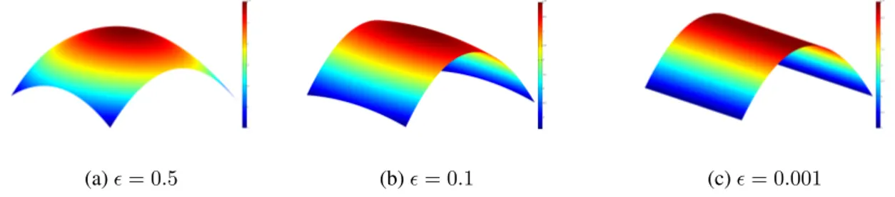
and Ri_{are the parameters of the Gaussian} hi_M as described in equation (2.8). Figure2.5represents an approximation of another part of the real map with a sum of 3 Gaussians.

Figure 2.5: Representation of a part of the real map and one possible approximation by a sum of Gaussians

The main advantage of polynomial maps is their potential to represent complicated real maps through local or global interpolation and/or approximation while adding relatively simple nonlinearities in the

(25)

system as shown in Figure 2.3 and2.4. The main advantage of using Gaussian maps is to represent multimodal maps, with several hills or peaks for instance as in Figure2.5 with potentially one global approximation. However, Gaussian maps introduces non polynomial nonlinearity in the observation equation which makes observer design in this case very complex.

We also study with less detail the case of a map decomposed in spatial trigonometric functions.

Figure 2.6: Fourier approximation of the real terrain with ntri= 1600

• A spatial trigonometric function:

hM(x1, x2) = αcos(ω1x1+ φ1)cos(ω2x2+ φ2) (2.10) where α ∈ R is a Fourier coefficient, (ω1, ω2) ∈ (R+)2 are pulsations and (φ1, φ2) ∈ R2are the phases at the origin.

• A sum of spatial trigonometric functions:

hi_M(x1, x2) = αicos(ωi1x1+ φi1)cos(ωi2x2+ φi2) hM = ntri X i=1 hi_M, (2.11)

where ntri ≥ 2, for i = 1, .., ntri, αi, (ω1i, ω2i)and (φi1, φi2)are the parameters of trigonometric functions as in equation (2.10). Figure2.6represents a Fourier approximation of the map in Figure

2.2with 1600 pulsations (ωi 1, ω2i).

As for polynomial maps, it is well known that the potential of approximation of such maps is huge but dealing with the cosines in the dynamics is a big issue in observer design. That is why, the full treatment of this case is still open.

(26)

Actually, a problem of observability arises with the observation equation (2.4) and (2.5) as one wants to reconstruct a 3D position with a 2D measurement or a 2D horizontal position with a 1D measurement. Therefore, the first step of the study is to look for conditions on the input and on the map of the ground that makes the state observable.

2.2.2 Local weak observability of Terrain-Aided Navigation models

In this section, we fix a position X, a speed V and an acceleration U. Depending on the dynamics considered in the following, X is a point in the statespace and V a constant input or (X, V ) is a point in the statespace and U a constant input. To check if a model is locally weakly observable, we evaluate the observability rank condition. To do so, The idea is to compute all the functions from the observation space OU(h)(or OV(h)) by successively applying the Lie derivative on the component of the observation function.

We focus on model (2.4) and we split the observation equation into a linear part hl_{and nonlinear part} hnl such that: h(X, V ) =„h nl_{(X, V )} hl(X, V )  , with hnl_{(X) = x} 3− hM(x1, x2)and hl(X, V ) = V.

In the case of a double integrator, as the linear part is directly of the speed, its Lie derivatives are constant so the only difficulty comes from the nonlinear part. We denote by hnl

k the kthLie derivative of hnl in the direction of the dynamics considered. Then, hnl₀ = hnl. Finally one only needs to check the rank of the family `∇hl_{, ∇h}nl

k ˘

k≥0where ∇ is the gradient operator.

2.2.2.1 Polynomial map of degree 2

We consider the dynamical model (2.3) of the double integrator with the observation equation2.4and the map (2.6) which is polynomial of degree 2. The successive Lie derivatives of hnl_{up to order 2 read:}

∇hnl₀ = » — — — — — — – −(2a₂₀x1+ a11x2+ a10) −(a₁₁x1+ 2a02x2+ a01) 1 0 0 0 fi ffi ffi ffi ffi ffi ffi fl , hnl₁ =∇Thnl₀ „V U  , = − v1(2a20x1+ a11x2+ a10) − v2(a11x1+ 2a02x2+ a01) + v3,

(27)

18 CHAPTER 2. TERRAIN MODELS AND OBSERVABILITY CONDITIONS ∇hnl₁ = » — — — — — — – −(2a20v1+ a11v2) −(a₁₁v1+ 2a02v2) 0 −(2a20x1+ a11x2+ a10) −(a₁₁x1+ 2a02x2+ a01) 1 fi ffi ffi ffi ffi ffi ffi fl , hnl₂ =∇Thnl₁ „V U  , = − v1(2a20v1+ a11v2) − v2(a11v1+ 2a02v2) − u₁(2a20x1+ a11x2+ a10) − u2(a11x1+ 2a02x2+ a01) + u3, ∇hnl 2 = » — — — — — — – −(2a₂₀u1+ a11u2) −(a11u1+ 2a02u2) 0 −(4a₂₀v1+ 2a11v2) −(2a11v1+ 4a02v2) 0 fi ffi ffi ffi ffi ffi ffi fl .

We then define the observability matrix H by:

H = » — — — — — — –

0 0 0 −(2a20x1+ a11x2+ a10) −(2a20v1+ a11v2) −(2a20u1+ a11u2) 0 0 0 −(a₁₁x1+ 2a02x2+ a01) −(a11v1+ 2a02v2) −(a11u1+ 2a02u2)

0 0 0 1 0 0 1 0 0 0 −(2a20x1+ a11x2+ a10) −(4a20v1+ 2a11v2) 0 1 0 0 −(a₁₁x1+ 2a02x2+ a01) −(2a11v1+ 4a02v2) 0 0 1 0 1 0 fi ffi ffi ffi ffi ffi ffi fl .

It is not necessary to compute the other Lie derivatives of h because one can see that they do not depend on X so their gradient do not bring vectors that are linearly independent of those of H as V is fully measured. Therefore, as H is a square matrix, the observability conditions can be summed up in the determinant of H. Finally, det(H) = −(2a20v1+ a11v2) −(2a20u1+ a11u2) −(a11v1+ 2a02v2) −(a11u1+ 2a02u2) ,

=(2a20v1+ a11v2)(a11u1+ 2a02u2) − (2a20u1+ a11u2)(a11v1+ 2a02v2), =2a20a11v1u1+ 4a20a02v1u2+ a211v2u1+ 2a11a02v2u2,

−(2a₂₀a11u1v1+ 4a20a02u1v2+ a211u2v1+ 2a11a02u2v2), =(a2₁₁v2− 4a20a02v2)u1+ (4a20a02v1− a211v1)u2, =(a2₁₁− 4a₂₀a02)(u1v2− u2v1).

Then,

dim`dOU(h)|(X,V )˘ < 6 ⇔det(H) = 0 ⇔ (a211− 4a20a02) det

ˆ„u1 v1 u2 v2 ˙ = 0, ⇔ a2₁₁− 4a20a02= 0or „u1 u2  //„v1 v2  .

(28)

Finally, in this case, the rank condition is satisfied if: • a2

11− 4a20a026= 0which means that the quadrics that corresponds to the map is non degenerate; • and the horizontal acceleration is chosen to be non colinear to the horizontal speed.

The case of a cubic polynomial leads to similar sufficient conditions involving higher order coeffi-cients so we omit the details of the computations.

2.2.2.2 Gaussian map

We analyse now the case of the Gaussian map (2.8). we consider successively dynamics (2.2) and (2.3) to get a progressive insight because the conditions are less clear than in the polynomial case. Let us set:

Xce= „x1− x01 x2− x02  , V12= „v1 v2  .

Xce represents the horizontal position centred at the centre of the Gaussian and V12 is the horizontal speed. We first notice that: ∇(x1,x2)hM = −hMRXce. We start with the simple integrator.

Simple integrator

In this case, as V is an input h = h0 = hnl = x3− hM. We compute several Lie derivatives:

∇hnl₀ =„hMRXce 1  , (2.12) hnl₁ = ∇hnl₀ V, = v3+ XceTRV12hM, ∇hnl₁ = hM„−(X T ceRV12)RXce+ RV12 0  , (2.13) hnl₂ = ∇Thnl₁ V, = hM(−(XceTRV12) 2 + V₁₂TRV12), ∇hnl₂ = hM „ −(−(XT ceRV12) 2 + V₁₂TRV12)RXce− 2(XceTRV12)RV12 0  , hnl₃ = ∇Thnl₂ V, = hM((XceTRV12) 3 − 3(V₁₂TRV12)(XceTRV12)), ∇hnl₃ = hM „ −((XT ceRV12)3− 3(V12TRV12)(XceTRV12))RXce+ (3(XceTRV12)2− V12TRV12)RV12 0  . (2.14) One can see from the previous computations that some structure appears in the Lie derivatives which leads to Proposition2.3.

Proposition 2.3. ∀k ≥ 1, there exist polynomial functions gk : R2−→ R and fk: R −→ R such that: hnl_k(X, hM, V ) = fk(v3) + hM(gk(V12TRV12, XceTRV12)),

(29)

and ∀(r, s) ∈ R+_{× R, g}

k(r, s)of degree k in s. Moreover, the following formula holds for the functions gk, ∀(r, s) ∈ R+× R and for k ≥ 1:

g1(r, s) = s,

gk+1(r, s) = −gk(r, s)s + ∂gk

∂s (r, s)r.

Proof. The proposition is true for k = 1 according to equation (2.13) with g1(r, s) = sand f1(v3) = v3 Let us assume that, for some n ≥ 1, there exists gk: R2−→ R and fk: R −→ R such that:

hnl_k (X, V ) = fk(v3) + hM(gk(V12TRV12, XceTRV12)) Then by definition, hnl_k+1 = VT∇hnl_k. Moreover, ∇hnl k = hM „−g_k(V₁₂TRV12, XceTRV12)RXce+ ∂g_∂sk(V12TRV12, XceTRV12)RV12 0  . (2.15) Finally, hnl_k+1= hM(−(XceTRV12)gk(V12TRV12, XceTRV12) + ∂gk ∂s (V T 12RV12, XceTRV12)V12TRV12). By setting, fk+1 = 0and gk+1(r, s) = −gk(r, s)s +∂g_∂sk(r, s)r, and by noticing that if gkis of degree kis s then gk+1is of degree k + 1 in s, the result is proved ∀k ≥ 1.

We can deduce from Proposition2.3and equation (2.12) that: dOV(h)|X=Span ˆ„−hMRXce 1  ,„−hM((X T ceRV12)RXce+ RV12) 0  , (2.16) ˆ„ hMgk(V12TRV12, XceTRV12)RXce+ hM∂g_∂sk(V12TRV12, XceTRV12)RV12 0 ˙ k≥2 ¸ . Equation (2.16) leads to the following sufficient conditions of local weak observability.

Proposition 2.4. If Xceis not colinear to V12and ∃k ≥ 1, ∃l ≥ 1 such that k 6= l and: gk(V12TRV12, XceTRV12) gl(V12TRV12, XceTRV12) ∂gk ∂s(V12TRV12, XceTRV12) ∂g_∂sl(V12TRV12, XceTRV12) 6= 0. (2.17)

then the system (2.2), (2.8) is locally weakly observable at X with input V .

Proof. The idea is to prove that the rank condition is verified at X with input V using the general form

of dOV(h)|X in equation2.16. To do so, we pick k and l form the statement of the proposition and we compute the following determinant:

D : = −h_MRxce hMgkRXce+ hM∂g_∂skRV12 hMglRXce+ hM∂g_∂slRV12 1 0 0 , D =h_Mg_kRX_ce+ h_M∂gk ∂s RV12 hMglRXce+ hM ∂gl ∂sRV12 , D = h2_mdet(R)det `“Xce V12 ‰˘ gk gl ∂gk ∂s ∂gl ∂s .

(30)

By construction, hM > 0and det(R) > 0. Besides, by assumption, Xce and V12are not colinear so det `“Xce V12‰˘ 6= 0and gk gl ∂gk ∂s ∂gl ∂s 6= 0.

Finally, D 6= 0 and dim(dOV(h)|X) = 3which ensures that the system (2.2), (2.8) is locally weakly observable at X with input V by Proposition2.1.

Equation (2.17) is verified for a generical choice of V12and U12as (V12TRV12, XceTRV12)is the root of some polynomial. Intuitively, Proposition2.4means that one can distinguish all 3D positions near X locally by going in straight line along a direction that is not parallel to Xce.We now deal with the case of a double integrator.

Double integrator

In this case, (X, V ) is the state and U the input. We define the horizontal acceleration as follows:

U12= „u1

u2 

.

As in the polynomial case the contribution of hl_{is easy to determine. Thus, we focus on h}nl_{. Like} in the simple integrator case one can derive the successive Lie derivatives:

hnl₀ = x3− hM, ∇hnl 0 = » — — — — – −hMRXce 1 0 0 0 fi ffi ffi ffi ffi fl , (2.18) hnl₁ = ∇Thnl₀ „V U  , (2.19) = v3+ XceTRV12hM, ∇hnl₁ = » — — — — – −hM(XceTRV12)RXce+ hMRV12 0 X_ceTRV12 hMRXce 1 fi ffi ffi ffi ffi fl , hnl₂ = ∇Thnl₁ „V U  , = hM(−(XceTRV12) 2 + V₁₂TRV12+ XceTRU12), (2.20)

(31)

22 CHAPTER 2. TERRAIN MODELS AND OBSERVABILITY CONDITIONS ∇hnl₂ = » — — – hM((−(XceTRV12) 2 + V₁₂TRV12+ XceTRU12)RXce− 2(XceTRV12)RV12+ RU12) 0 hM(2RV12− 2(XceTRV12)RXce) 1 fi ffi ffi fl , hnl₃ = ∇Thnl₂ „V U  , = hM((XceTRV12) 3 − 3(V₁₂TRV12)(XceTRV12) + 2U₁₂TRV12+ (1 − 2(XceTRV12))(XceTRU12)) + u3. (2.21) The expression of ∇hnl

3 becomes too long to be written here and as in the simple integrator, the Lie derivatives can be expressed in a general form with a sequence of multivariate polynomials.

Proposition 2.5. ∀k ≥ 1, there exist functions gk: R5−→ R and fk: R2 −→ R such that: hnl_k(X, V, U ) = fk(v3, u3) + hM(gk(V12TRV12, U12TRU12, XceTRV12, XceTRU12, V12TRU12)),

and ∀(ru, rv, sxv, sxu, svu) ∈ R+2×R3, gk(ru, rv, sxv, sxu, svu)is polynomial in (ru, rv, sxv, sxu, svu).

Moreover, a possible choice of the function sequence (gk)_k≥1is the one for which the following recursion

holds for , ∀(ru, rv, sxv, sxu, svu) ∈ R+2× R3and for k ≥ 1:

gk+1= −gksxv+ ∂gk ∂sxv rv+ ∂gk ∂svu ru+ ˆ ∂gk ∂sxu + 2∂gk ∂rv ˙ svu+ ∂gk ∂sxv sxu,

Proof. The proposition is true for k = 1 according to equation (2.19) with g1(ru, rv, sxv, sxu, svu) = sxv and f1(v3, u3) = v3

Let us assume that, for some k ≥ 1, there exists gk: R5 −→ R and fk: R2 −→ R such that: hnl_k (X, V ) = fk(v3, u3) + hMgk(V12TRV12, U12TRU12, XceTRV12, XceTRU12, V12TRU12). Then by definition, hnl_k+1 =“VT _UT_{‰ ∇h}nl k. Moreover, for k ≥ 1, ∇hnl_k = » — — — — – hM ´ −g_kRXce+ _∂s∂g_xvk RV12+_∂s∂g_xuk RU12 ¯ 0 hM ´ 2∂gk ∂rvRV12+ ∂gk ∂sxvRXce+ ∂gk ∂svuRU12 ¯ ∂fk ∂v3 fi ffi ffi ffi ffi fl . Then, hnl_k+1=hM ˆ −g_kX_ceTRV12+ ∂gk ∂sxv V₁₂TRV12+ ∂gk ∂sxu U₁₂TRV12+ 2∂gk ∂rv V₁₂TRU12+ ∂gk ∂sxv XceRU12+ ∂gk ∂svu U₁₂TRU12. + ∂fk ∂v3 u3 ˙ .

(32)

2.2. OBSERVABILITY PROPERTIES IN TERRAIN-AIDED NAVIGATION 23 By setting, gk+1= − gkXceTRV12+ ∂gk ∂sxv V₁₂TRV12+ ∂gk ∂sxu U₁₂TRV12 + 2∂gk ∂rv V₁₂TRU12+ ∂gk ∂sxv XceRU12+ ∂gk ∂svu U₁₂TRU12, fk+1= ∂fk ∂v3 u3, one gets the result.

From Proposition2.5, one gets directly that:

dOU(h)|(X,V )= Span ¨ ˚ ˚ ˚ ˚ ˚ ˚ ˝ » — — — — — — – 0 0 0 1 0 0 fi ffi ffi ffi ffi ffi ffi fl , » — — — — — — – 0 0 0 0 1 0 fi ffi ffi ffi ffi ffi ffi fl , » — — — — — — – 0 0 0 0 0 1 fi ffi ffi ffi ffi ffi ffi fl , » — — — — – −h_MRXce 1 0 0 0 fi ffi ffi ffi ffi fl , ¨ ˚ ˚ ˚ ˚ ˝ » — — — — – hM ´ −gkRXce+_∂s∂g_xvkRV12+ _∂s∂g_xuk RU12 ¯ 0 hM ´ ∂gk ∂sxvRXce+ 2 ∂gk ∂rvRV12+ ∂gk ∂svuRU12 ¯ ∂fk ∂v3 fi ffi ffi ffi ffi fl ˛ ‹ ‹ ‹ ‹ ‚ k≥1 ˛ ‹ ‹ ‹ ‹ ‹ ‚ . (2.22)

Suppose that V12is not colinear to U12. Let us define (xv, xu) as the coordinates of Xce in the basis formed by (V12, U12). We can now state the equivalent of Proposition2.5for the double integrator:

Proposition 2.6. If V12is not colinear to U12, ∃k ≥ 1, ∃l ≥ 1 such that k 6= l and: −xvgk+_∂s∂g_xvk −xvgl+_∂s∂g_xvl −xugk+_∂s∂g_vuk −xugl+_∂s∂g_vul 6= 0, (2.23)

the system (2.3), (2.8) is locally weakly observable at (X, V ) with input U.

Proof. Following the same reasoning as in Proposition2.3, one only needs to compute the following determinant: D : = −h_MRXce hM(−gkRXce+_∂s∂g_xvk RV12+_∂s∂g_xuk RU12) hM(−glRXce+ _∂s∂g_xvl RV12+_∂s∂g_xul RU12) 1 0 0 , D = h2_mdet(R)det `“V12 U12 ‰˘ −xvgk+_∂s∂g_xvk −xvgl+_∂s∂g_xvl −xugk+ ∂s∂gvuk −xugl+ ∂gl ∂svu .

As in proposition (2.3), D 6= 0 and the system (2.3), (2.8) is locally weakly observable at (X, V ) with input U.

The property (2.23) is expected to be verified generically as (2.17). The property that V12 and U12 must not be colinear is more useful than its counterpart in the simple integrator case as both V12and U12 are known. It is not surprising as more information is available in the double integrator case than in the simple integrator one. It also matches the condition in the polynomial case.

(33)

2.2.2.3 Map as a sum of Gaussian

Let us set: X_cei =„x1− x i 1 x2− xi2  . We recall that: h(X, V ) =„h nl_{(X, V )} hl(X, V )  , with hnl_{(X) = x} 3−Pn_i=1g hi_M(x1, x2)and hl(X, V ) = V. We first notice that ∇(x1,x2)h

i M = −hiMRiXcei . Simple integrator ∇hnl₀ = „Png i=1hiMRiXcei 1  , (2.24) hnl₁ = ∇Thnl₀ V, = v3+ ng X i=1 hi_MX_ceiTRiV12, (2.25) (2.26) Following the same path as in the case of one Gaussian, proposition (2.7) is stated as follows.

Proposition 2.7. ∀k ≥ 1, ∃ gk: R2 −→ R and fk : R −→ R such that:

hnl_k(X, V ) = fk(v3) + ng X i=1 hi_M(gk(V12TRiV12, XceiTRiV12)), and ∀(r, s) ∈ R+_{× R, g}

k(r, s)is polynomial in (r, s) in s. Besides, gk(r, s)is of degree n. Moreover,

the following recursion holds for the functions gk, ∀(r, s) ∈ R+× R and for n ≥ 1:

gk+1(r, s) = −gk(r, s)s + ∂gk

∂s (r, s)r

Proof. The proposition is true for k = 1 according to equation (2.25) with g1(r, s) = sand f1(v3) = v3 Let us assume that, for some k ≥ 1, there exists gk: R2 −→ R and fk: R −→ R such that:

hnl_k(X, V ) = fk(v3) + ng X i=1 hi_M(gk(V12TRiV12, XceiTRiV12)). Then by definition, hnl_k+1 = VT∇hnl_k.

(34)

To simplify the notations we denote gk(V12TRiV12, XceiTRiV12)by g_ki and ∂g_∂sk(V12TRiV12, XceiTRiV12)by ∂gi k ∂s: ∇hnl_k = « −Png i=1gkiRiXcei + Png i=1hiM ∂gi k ∂s R i_V 12 0 ff . (2.27) Finally, hnl_k+1= ng X i=1 hi_M(−(X_ceiTRiV12)gik+ V12TRiV12 ∂gi k ∂s ).

By setting, fk+1= 0and gk+1(r, s) = −gk(r, s)s +∂g∂sk(r, s)r, and by noticing that if gkis of degree nis s then gk+1is of degree k + 1 in s, the result is proved ∀k ≥ 1.

By equations and (2.24) and (2.27), one can see that:

dOU(h)|X= Span ¨ ˝ „Png i=1hiMRiXcei 1  , ˜« −Png i=1gkiRiXcei + Png i=1hiM ∂gi k ∂s R i_V 12 0 ff¸ n≥1 ˛ ‚. (2.28) Simple analytic conditions for local weak observability in this case are harder to provide as the directions spanned by ∇hnl

k are not a combination of Xce and V12 but a combination between the Xcei and V12. However, this new complexity seems beneficial, at least intuitively, as it means that more directions are spanned in the case of a sum of Gaussian than in the case of one Gaussian. For example, if ng = 2, R1 = R2, and X_ce1, X_ce2 and V12 are colinear then one can show that rank condition is not satisfied, using that the same technique as in the single Gaussian case. However, it is a very particular case, with many symmetries. It means notably that the drone is located on the line that connects the centres of the two Gaussians and goes in that direction too. Moreover, if the drone deviates from this line the rank condition is satisfied. This example illustrates the fact that the rank condition seems to fail only in very special cases.

Double integrator

Using the same notations as in the single Gaussian case:

hnl₀ = x3− ng X i=0 hi_M, ∇hnl₀ = » — — — — – −Png i=0hiMRiXcei 1 0 0 0 fi ffi ffi ffi ffi fl , (2.29)

(35)

26 CHAPTER 2. TERRAIN MODELS AND OBSERVABILITY CONDITIONS hnl₁ = ∇Thnl₀ „V U  , (2.30) = v3+ ng X i=0 X_ceiTRiV12hiM, ∇hnl₁ = » — — – −Png i=0h1M(XceiTRiV12)RiXcei + Png i=0hiMRiV12 0 Png i=0hiMRiXcei 1 fi ffi ffi fl . (2.31)

Proposition 2.8. ∀k ≥ 1, ∃ gk: R5 −→ R and fk : R2 −→ R such that:

hnl_k(X, V, U ) = fk(v3, u3) + ng X i=0 hi_M(gk(V12TRiV12, U12TRiU12, XceiTRiV12, XceiTRiU12, V12TRiU12)). and ∀(ru, rv, sxv, sxu, svu) ∈ (R+)2×R3, gk(ru, rv, sxv, sxu, svu)is polynomial in (ru, rv, sxv, sxu, svu).

Moreover, a possible choice of the function sequence (gk)k≥1is the one for which the following recursion

holds for , ∀(ru, rv, sxv, sxu, svu) ∈ R+2× R3and for k ≥ 1:

gk+1= −gksxv+ ∂gk ∂sxv rv+ ∂gk ∂svu ru+ ˆ ∂gk ∂sxu + 2∂gk ∂rv ˙ svu+ ∂gk ∂sxv sxu.

Proof. The proposition is true for k = 1 according to equation (2.19) with g1(ru, rv, sxv, sxu, svu) = sxv and f1(v3, u3) = v3

Let us assume that, for some k ≥ 1, there exists gk: R5 −→ R and fk: R2 −→ R such that:

hnl_k(X, V, U ) = fk(v3, u3) + ng X i=0 hi_M(gk(V12TRiV12, U12TRiU12, XceiTRiV12, XceiTRiU12, V12TRiU12)). Then by definition, hnl_k+1 =“VT UT‰ ∇hnl_k. Moreover, for k ≥ 1, ∇hnl k = » — — — — – −Png i=0hiMgkiRiXcei + Png i=0hiM ∂gi k ∂sxvR i_V 12+Pni=0g hiM ∂gi k ∂sxuR i_U 12 0 Png i=0hiM ∂gi k ∂sxvR i_Xi ce+ 2 Png i=0hiM ∂gi k ∂rvR i_V 12+P ng i=0hiM ∂gi k ∂svuR i_U 12 ∂fk ∂v3 fi ffi ffi ffi ffi fl .

The result follows as in (2.5), by setting, ∀(ru, rv, sxv, sxu, svu) ∈ R+2× R3and for k ≥ 1:

gk+1= −gksxv+ ∂gk ∂sxv rv+ ∂gk ∂svu ru+ ˆ ∂gk ∂sxu + 2∂gk ∂rv ˙ svu+ ∂gk ∂sxv sxu.

(36)

From proposition (2.8), one gets directly that:

dOU(h)|(X,V )=Span ¨ ˚ ˚ ˚ ˚ ˚ ˚ ˝ » — — — — — — – 0 0 0 1 0 0 fi ffi ffi ffi ffi ffi ffi fl , » — — — — — — – 0 0 0 0 1 0 fi ffi ffi ffi ffi ffi ffi fl , » — — — — — — – 0 0 0 0 0 1 fi ffi ffi ffi ffi ffi ffi fl , » — — — — – −Png i=0hiMRiXcei 1 0 0 0 fi ffi ffi ffi ffi fl , ¨ ˚ ˚ ˚ ˚ ˝ » — — — — – −Png i=0hiMgkiRiXcei + Png i=0hiM ∂gi k ∂sxvR i_V 12+Pni=0g hiM ∂gi k ∂sxuR i_U 12 0 Png i=0hiM ∂gi k ∂sxvR i_Xi ce+ 2 Png i=0hiM ∂gi k ∂rvR i_V 12+P ng i=0hiM ∂gi k ∂svuR i_U 12 ∂fk ∂v3 fi ffi ffi ffi ffi fl ˛ ‹ ‹ ‹ ‹ ‚ k≥1 ˛ ‹ ‹ ‹ ‹ ‚ . (2.32) As in the previous cases, the rank condition will be verified for a generical choice of vector V12and U12 if the sum of Gaussian does not represent a pathological map, with concentric Gaussian for example.

The main conclusion that can be drawn from the study of the observability condition is that the more complex the map is the more information it contains and the more likely it is to lead to observable systems. It confirms the previous informal claim However, the conditions presented in this section, especially on the control, are qualitative but not quantitative. They give a good insight on the nature of the problem but no practical resolution scheme.

The goal of the next chapter is to find more quantitative and applicable conditions through observer and controller design.

(37)

(38)

Chapter 3

Observer and controller design for TAN

with analytical maps under persistence of

excitation

This chapter is firstly dedicated to observer design for the systems studied in Chapter2. Actually, it turns out that these observers converge under a condition of persistence of excitation on the speed. This implies that there are also conditions on the control to ensure the convergence of the observer . Therefore, the second goal of this chapter is to design controllers that simultaneously verify these conditions and allow the system to reach his guiding objective. Finally, we study quite independently a special case of stochastic persistent horizontal speed.

3.1 Nonlinear observer design by Immersion and Invariance (I&I) for

Terrain-Aided Navigation

Generally, an observer is defined as a dynamical system designed to asymptotically approach the un-known state of the original system. The main difficulty is that it must be constructed using only the avail-able information.There is no explicit form of observers that handles any system so it must be adapted to the particular class of systems treated. The most popular nonlinear observer are the nonlinear Luenberger and Kalman observers. They are especially well suited for a large class of nonlinear systems that still ex-hibit some linear structure (see [Besançon, 2007]). Another family of nonlinear observers are high-gain observers. They are based on the idea of compensating the nonlinearity buy using a high gain on the innovation term. This also requires in general that the original system contains a linear detectable part (see [Khalil and Praly, 2014]). In the sequel, we prefer to use a more general method, called Immersion and Invariance (I&I), that is known to be able to deal with very nonlinear systems. Besides, it gives one many degrees of freedom to choose the estimation error equation. In this section, we first recall the gen-eral concepts of I&I applied to observer design. Then, we present the design of observers for the systems with a quadratic map, a cubic map, a Gaussian map and a trigonometric map.