Analyse de grappe des données de catégories et de séquences étude et application à la prédiction de la faillite personnelle

Analyse de grappe des donnees de categories et de sequences

etude et application a la prediction de la faillite personnelle

par

Tengke Xiong

these presentee au Departement d'informatique

en vue de I'obtention du grade de philosophiae doctor (Ph.D.)

FACULTE DES SCIENCES

UNIVERSITE DE SHERBROOKE

HI

Your file Votre reference ISBN: 978-0-494-83344-5 Our file Notre reference ISBN: 978-0-494-83344-5

NOTICE:

The author has granted a

non-exclusive license allowing Library and Archives Canada to reproduce, publish, archive, preserve, conserve, communicate to the public by

telecommunication or on the Internet, loan, distrbute and sell theses

worldwide, for commercial or non-commercial purposes, in microform, paper, electronic and/or any other formats.

AVIS:

L'auteur a accorde une licence non exclusive permettant a la Bibliotheque et Archives Canada de reproduire, publier, archiver, sauvegarder, conserver, transmettre au public par telecommunication ou par I'lnternet, prdter, distribuer et vendre des theses partout dans le monde, a des fins commerciales ou autres, sur support microforme, papier, electronique et/ou autres formats.

The author retains copyright ownership and moral rights in this thesis. Neither the thesis nor substantial extracts from it may be printed or otherwise reproduced without the author's permission.

L'auteur conserve la propriete du droit d'auteur et des droits moraux qui protege cette these. Ni la these ni des extraits substantiels de celle-ci ne doivent etre imprimes ou autrement

reproduits sans son autorisation.

In compliance with the Canadian Privacy Act some supporting forms may have been removed from this thesis.

While these forms may be included in the document page count, their removal does not represent any loss of content from the thesis.

Conformement a la loi canadienne sur la protection de la vie privee, quelques formulaires secondares ont ete enleves de cette these.

Bien que ces formulaires aient inclus dans la pagination, il n'y aura aucun contenu manquant.

CLUSTERING CATEGORICAL AND SEQUENCE DATA:

INVESTIGATION AND APPLICATION IN PERSONAL

BANKRUPTCY PREDICTION

Tengke Xiong

Faculte des Sciences

Universite de Sherbrooke

A thesis submitted for the degree of

Doctor of Philosophy

Le23juin2011

lejury a accept e la these de Monsieur Tengke Xiong dans sa version finale.

Membres du jury

Professeur Shengrui Wang Directeur de recherche Departement d'informatique

Professeur Andre Mayers Codirecteur de recherche Departement d'informatique

Professeur Ernest Monga Evaluateur externe au programme

Departement de mathematiques

Professeur Aijun An Evaluateur externe

Department of Computer Science and Engineering York University

Professeur Pierre-Marc Jodoin President rapporteur Departement d'informatique

Acknowledgements

First and foremost, I am grateful to my advisors Shengrui Wang and Andre Mayers. I have benefited so much in my research from the inspiration, motivation and encour-agement that Prof. Wang constantly provided in the past four years. Prof. Mayers was always patient and gave me a lot of valuable advise and instruction. Working with them was really memorable and fun experience.

I also would like to thank Prof. Ernest Monga. Prof. Monga provided valuable suggestion on the project of personal bankruptcy prediction, I learned a lot from the discussion with him. Thanks are specially due to Vincent for his cooperation and help on the project.

I would like to thank my thesis committee members for giving me extremely valuable feedback on my thesis, their reviews and comments are really helpful to improve the thesis.

I would like to thank all my friends at UdeS, they made my years in Sherbrooke a fantastic experience.

Part of the research work presented in this thesis was supported by the Natural Sciences and Engineering Research Council of Canada (NSERC) Collaborative Re-search and Development (CRD) Grant. I was financially supported by the scholarship obtained from the NSERC CRD project and research funds of Prof. Wang during my studies at the Universite de Sherbrooke. I would like to express my sincere thanks to NSERC.

Finally, I would like to thank my family for their unconditional and untiring support and contribution. I could not finish my degree without my family. Their love is my worthless treasure.

S o m m a i r e

L'analyse de grappes est l'une des techniques les plus importantes utilisees dans le forage de donnees. Elle a de nombreuses applications dans I'extraction de motifs, la recherche d'information, la synthese d'information, la compression, etc. Les travaux de recherche de cette these portent sur le regroupement des donnees categoriques et sequentielles. II s'agit d'une tache beaucoup plus difficile que le regroupement des donnees numeriques, due au manque de mesure de similarite evidente entre les donnees categoriques et entre les sequences categoriques. Dans cette these, nous avons con^u des algorithmes efncaces pour regrouper des donnees et des sequences categoriques. Nos etudes experiment ales permettent de demontrer les performances superieures de nos algorithmes par rapport aux algorithmes existants. Nous avons aussi applique des algorithmes proposes pour resoudre le probeme de prediction de la faillite personnelle.

Le regroupement des donnees categoriques pose deux defis : definir une mesure de similarite significative, et traiter efncacement les groupes qui resident dans des sous-espaces differents. Dans cette these, nous considerons l'analyse de grappes dans une perspective d'optimisation et proposons une nouvelle fonction objectif. En se basant sur cette formulation, nous concevons un nouvel algorithme hierarchique par divi-sion, nomrne DHCC, pour les donnees categoriques. Dans la procedure de bisection du DHCC, l'initialisation de la division est basee sur l'analyse des correspondances multiples (ACM). Nous elaborons une strategie pour pallier a un probleme cle de l'approche par division, a savoir quand il n'est plus necessaire de diviser. L'algorithme propose est entierement automatique (sans parametre, aucune hypothese concernant le nombre de groupes), independant de l'ordre dans lequel les donnees sont traitees,

extensible a de grands ensembles de donnees, et finalement. capable de decouvrir naturellement des groupes inclus dans des sous-espaces.

La connaissance a priori sur les donnees peut etre incorporee dans le processus de l'analyse de grappes, ce qui est connu sous de nom de 1'analyse de grappes semi-supervisee, pour procurer une amelioration considerable pour la qualite de l'analyse de grappes. Dans cette these, nous considerons l'analyse de grappes semi-supervisee comme un probleme d'optimisation avec contraintes au niveau des instances et pro-posons une approche automatique pour guider le processus de l'optimisation sous contraintes. Ceci nous permet de proposer un nouvel algorithme semi-supervise hierarchique par division pour les donnees categoriques, nomine SDHCC. Notre al-gorithme ne necessite pas la fixation de parametre, ne comporte aucune operation sensible a l'ordre de traitement de donnees et est efficace en prenant l'avantage des connaissances au niveau de contraintes d'appartenance des instances pour ameliorer la qualite des resultats.

De nombreux algorithmes de regroupement des sequences s'appuient sur une mesure de similitude entre des paires de sequences. Habituellement, une telle mesure est efficace s'il y a beaucoup d'informations dans les motifs retrouves parmi ces sequences. Toutefois, il est difficile de definir une mesure de similar ite significative pour les paires de sequences si celles-ci sont courtes et contiennent du bruit. Dans cette these, nous contournons cet obstacle en definissant une mesure de similitude entre une sequence individuelle et un ensemble de sequences en se basant sur un modele de la distribution de probability conditionnelle. A partir de cette mesure, nous concevons un nouvel algorithme X-moyennes base sur le modele pour T analyse de grappes de sequences. Cet algorithme fonctionne de fac,on similaire au traditionnel algorithme X-moyennes pour les donnees vectorielles.

Enfin, nous avons developpe un systeme pour la prediction de faillites person-nelles dont les attributs de predictions sont principalement les attributs de faillites decouverts par les techniques de regroupement proposes dans cette these. Les car-acteristiques de faillites decouvertes sont representees dans un espace vectoriel de basses dimensions. A partir du nouvel espace d'attributs, qui peut etre complete avec des attributs existants de prediction connus (par exemple, le score de credit),

un classincateur base sur la machine a vecteur de support (SVM) est developpe pour combiner ces difierents attributs. Les resultats experimentaux demontrent que notre systeme est prometteur pour la prediction au niveau de la performance et au niveau de I'explication qu"il peut fournir.

Abstract

Cluster analysis is one of the most important and useful data mining techniques, and there are many applications of cluster analysis in pattern extraction, information retrieval, summarization, compression and other areas. The focus of this thesis is on clustering categorical and sequence data. Clustering categorical and sequence data is much more challenging than clustering numeric data because there is no inherently meaningful measure of similarity between the categorical objects and sequences. In this thesis, we design novel efficient and effective clustering algorithms for clustering categorical data and sequence respectively, and we perform extensive experiments to demonstrate the superior performance of our proposed algorithm. We also explore the extent to which the use of the proposed clustering algorithms can help to solve the personal bankruptcy prediction problem.

Clustering categorical data poses two challenges: defining an inherently meaning-ful similarity measure, and effectively dealing with clusters which are often embedded in different subspaces. In this thesis, we view the task of clustering categorical data from an optimization perspective and propose a novel objective function. Based on the new formulation, we design a divisive hierarchical clustering algorithm for cate-gorical data, named DHCC. In the bisection procedure of DHCC, the initialization of the splitting is based on multiple correspondence analysis (MCA). We devise a strategy for dealing with the key issue in the divisive approach, namely, when to ter-minate the splitting process. The proposed algorithm is parameter-free, independent of the order in which the data is processed, scalable to large data sets and capable of seamlessly discovering clusters embedded in subspaces.

The prior knowledge about the data can be incorporated into the clustering pro-cess, which is known as semi-supervised clustering, to produce considerable improve-ment in learning accuracy. In this thesis, we view semi-supervised clustering of cat-egorical data as an optimization problem with extra instance-level constraints, and propose a systematic and fully automated approach to guide the optimization process to a better solution in terms of satisfying the constraints, which would also be benefi-cial to the unconstrained objects. The proposed semi-supervised divisive hierarchical clustering algorithm for categorical data, named SDHCC, is parameter-free, fully automatic and effective in taking advantage of instance-level constraint background knowledge to improve the quality of the resultant dendrogram.

Many existing sequence clustering algorithms rely on a pair-wise measure of simi-larity between sequences. Usually, such a measure is effective if there are significantly informative patterns in the sequences. However, it is difficult to define a meaningful pair-wise similarity measure if sequences are short and contain noise. In this thesis, we circumvent the obstacle of defining the pairwise similarity by defining the similarity between an individual sequence and a set of sequences. Based on the new similarity measure, which is based on the conditional probability distribution (CPD) model, we design a novel model-based K-me&ns clustering algorithm for sequence clustering, which works in a similar way to the traditional /C-means on vectorial data.

Finally, we develop a personal bankruptcy prediction system whose predictors are mainly the bankruptcy features discovered by the clustering techniques proposed in this thesis. The mined bankruptcy features are represented in low-dimensional vec-tor space. From the new feature space, which can be extended with some existing prediction-capable features (e.g., credit score), a support vector machine (SVM) clas-sifier is built to combine these mined and already existing features. Our system is readily comprehensible and demonstrates promising prediction performance.

Contents

1.3.1 Clustering categorical data 6 1.3.2 Clustering sequence data 8 1.4 Personal bankruptcy prediction 9

1.5 Thesis contributions 10

2 Clustering Categorical Data 12

2.1 Introduction 12 2.2 Related work 13 2.3 Notation and definitions 18

2.4 MCA calculation on indicator matrix 18 2.5 Optimization perspective for clustering categorical data 23

2.6.1 Preliminary splitting 27

2.6.2 Refinement 28 2.6.3 Termination of splitting process 29

2.6.4 Subspace clustering 31 2.6.5 Algorithm analysis 33 2.7 Experimental results 34 2.7.1 Quality measures 35 2.7.2 Synthetic data 37 2.7.3 Real-life data 42 2.8 Chapter summary 47

3 Semi-supervised Clustering of Categorical D a t a 50

3.1 Introduction 50 3.2 Related work 51 3.3 Notation and definitions 53

3.4 Semi-supervised DHCC 55 3.4.1 Initialization 56 3.4.2 Refinement 57 3.4.3 Alleviation of cannot-link violation 60

3.5 Experimental results 62 3.5.1 Evaluation measure and methodology 63

3.5.2 Results and discussion 64

3.6 Chapter summary 71

4 Clustering Sequence Data 72

4.1 Introduction 72 4.2 Related work 73 4.3 A new measure of similarity between a categorical sequence and a cluster 75

4.4 Calculation of the new measure 77

4.5 Model-based A'-means 80 4.6 Experimental results 83 4.7 Chapter summary 87

5 Personal Bankruptcy Prediction 88

5.1 Introduction 88 5.2 Related work 90 5.3 Feature mining from categorical data 92

5.4 Feature mining from sequence data 94

5.4.1 Motivation 94 5.4.2 Sequence representation of client behavior 95

5.4.3 Modification and extension of the CPD model 96

5.4.4 Sequence pattern extraction 99 5.5 Bankruptcy feature representation 101

5.6 Prediction results 102 5.6.1 Feature mining 104 5.6.2 Final prediction system 110

5.7 Chapter summary I l l

6 Conclusions and Future Work 113

List of Figures

1.1 Agglomerative hierarchical clustering algorithm 3

1.2 Basic /('-means algorithm 5 1.3 The relationship between debt and period before bankruptcy 10

2.1 Scheme of DHCC 26 2.2 Symmetric correspondence analysis map of scenario data 28

2.3 Algorithm of refining the preliminary bisection 29

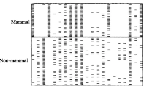
2.4 Incidence matrix of bisection of Zoo 32 2.5 Comparison of DHCC in terms of NMI on synthetic data 39

2.6 Scalability with respect to data size 41 2.7 Scalability with respect to dimensionality 42 2.8 Comparison of DHCC in terms of NMI on real-life data 49

3.1 COP-KMEANS algorithm 53 3.2 Constraint closures generated from instance-level constraints 54

3.3 The framework of the bisection procedure of SDHCC 56

3.4 Algorithm of the second step of SDHCC 59 3.5 Algorithm of the third step of SDHCC 61

3.6 Algorithm of Divide-Cluster 62 3.7 Algorithm of Merge-Clusters 62 3.8 Semi-supervised clustering results on Zoo data set 65

3.9 Semi-supervised clustering results on Votes data set 66 3.10 Semi-supervised clustering results on Cancers data set 66 3.11 Semi-supervised clustering results on Mushroom data set 67

3.12 Semi-supervised clustering results on Similar-2 data set 69 3.13 Semi-supervised clustering results on different-3 data set 69

4.1 Flowchat of the CLUSEQ algorithm 76

4.2 A probabilistic suffix tree 79 4.3 Model-based i\T-means for categorical sequences 81

4.4 Mean precision and variation on protein data 84 4.5 Mean recall and variation on protein data 85

5.1 Framework of our prediction system 90 5.2 Categorical table built from credit card data 93

5.3 Decomposition of an ordinal sequence 98 5.4 Samples drawn from two bankruptcy clusters 100

5.5 Samples drawn from two non-bankruptcy clusters 100 5.6 The distribution of identified bad accounts over the prediction period 106

5.7 ROC curve for case identification 106 5.8 ROC curve of March 2006 balance of identified bad accounts 108

5.9 ROC curve of balance of identified bad accounts when bankruptcy

Chapter 1

Introduction

Cluster analysis is one of the most important and useful data mining techniques [32, 37, 46, 77]. Clustering is an exploratory learning process whose aim is to group unlabeled data into meaningful clusters, so that objects in the same cluster show great similarity and objects from distinct clusters show great dissimilarity. The con-cept of similarity can be defined in many different ways, according to the purpose of the; analysis, domain-specific assumption and prior background knowledge about the data. There are many applications of cluster analysis in pattern extraction, informa-tion retrieval, summarizainforma-tion, compression and other areas. Most of the clustering algorithms present in the literature focus on data sets where the objects are defined on a set of numerical values. In such a case, the similarity of the objects can be decided using well-studied measures derived from geometric analogies, such as Euclidean dis-tance. While categorical data is commonly seen in many real-life applications, where the elements of the data are non-numeric and nominal, imposing more challenge for cluster analysis in these domains.

The investigation of clustering categorical and sequence data arises from our project on a major Canadian bank. In our project, original high-dimensional complex data are transformed into categorical data, which mainly takes two forms: categorical tuples and sequences. We resort to clustering techniques to discover the comprehensi-ble features that can distinguish bad accounts from good ones. The focus of this thesis is on clustering categorical and sequence data, and the application of the proposed

clustering techniques in personal bankruptcy prediction. In this chapter, we will give an overview of traditional unsupervised and semi-supervised learning, and then de-scribe the clustering method for categorical and sequence data, and then present an introduction to personal bankruptcy prediction. We conclude this chapter with a discussion of the thesis contributions.

1.1 Unsupervised learning

Two of the most important tasks in the field of data mining are classification and clustering [30, 85]. Classification is a supervised learning technique, whereas cluster-ing is completely unsupervised. The aim of clustercluster-ing is to group a set of objects into clusters without the guidance of prior background knowledge. Clustering techniques are broadly divided into hierarchical and partitioning, depending on whether the al-gorithm generates a hierarchical clustering structure or a flat partition of the data set.

1.1.1 Hierarchical clustering

In hierarchical clustering, the objects are placed in different clusters, and these clusters have ancestor-descendant relationship. Usually, a binary tree is employed to represent the dendrogram structure of the clustering results. The dendrogram can be cut at different levels to generate different clustering of the data. Hierarchical clustering algorithms can be further divided into agglomerative (bottom-up) and divisive (top-down) methods:

• Agglomerative methods: Start with each object as a singleton cluster and, at each step, merge the closest pair of clusters according to the similarity measure. The most commonly used methods to measure the similarity between pairwise clusters are single-link, complete-link, and group average. Agglomerative meth-ods suffer from high time complexity and the problem that early wrong decision of merging two small clusters can expand to following merges, leading to unde-sirable final clustering tree structure. Fisher (1996) studied iterative hierarchical

cluster redistribution to improve once constructed dendrogram [33]. Karypis et al. (1999) also researched refinement for hierarchical clustering [48]. However, the global refinement procedure destroys the desirable hierarchical clustering structure [15, 90]. A basic agglomerative hierarchical clustering algorithm is illustrated in Figure 1.1.

• Divisive methods: Start with one, all-inclusive cluster containing all the objects and, at each step, split a cluster until only singleton clusters of individual objects remain or the termination criterion is satisfied. The two most important issues of divisive methods are how to split a cluster and how to choose the next cluster to split or when to terminate splitting (if not intending to generate the whole clustering tree).

Algorithm: Agglomerative Hierarchical Clustering

1. Place each object in its own cluster. Computer the prox-imity matrix containing the distance between each pair of objects.

2. Repeat until the number of clusters reaches one.

(a) Find the most similar pair of clusters Ct and Cj using

the proximity matrix. Merge clusters C, and Cj to a new cluster Cp.

(b) Remove Cj and Cj from current clusters, and update the proximity matrix by adding the distance between cluster Cp and other clusters.

Figure 1.1: Agglomerative hierarchical clustering algorithm

1.1.2 Partitioning clustering

In partitioning clustering, given a data set and the number of clusters K, an algorithm divides data into K subsets, in which, each subset represents a cluster. Partitioning

clustering is further divided into hard clustering and fuzzy clustering. In hard clus-tering, each object belongs to exactly one cluster. In fuzzy clusclus-tering, each object is allowed to belong to two or more clusters, associated with a set of membership degrees [43]. In this thesis, we only consider assigning each object to exactly one cluster.

Partitioning clustering exploits iterative relocation to optimize the partition of the data set. Unlike traditional hierarchical methods, in which clusters are not revisited after being constructed, an algorithm of partitioning clustering tries to discover the clusters by iteratively reassigning objects between the K clusters.

The number of clusters K is assumed as a prior known parameter in most par-titioning methods. Learning the 'true' number of clusters in a given data set is a fundamental and largely unsolved problem [75, 76]. In hierarchical clustering, this problem is less critical, as the hierarchical clustering structure offers more flexibil-ity to analyzing the data at different levels of similarflexibil-ity. A partition of the data in hierarchical clustering can be obtained by cutting the clustering tree at certain level. There are a number of techniques in partitioning clustering, we list some as fol-lows. In the center-based method, the most representative object within a cluster is selected to represent the cluster (A'-medoids [64]), or each cluster is represented by the mean of its objects, which is call centroid (A-means). In the density-based method, a cluster is defined as a connected dense component against surrounding region, a representative algorithm is DBSCAN [31]. In the probabilistic method, each object is considered to be a sample independently drawn from a mixture model of several probability distributions, and the Expectation-Maximization (EM) tech-nique is exploited to optimize the overall likelihood of generating the whole data set [73]. In the graph-theoretic method, the clustering problem is modeled by a graph

G = (V, E), where each vertex vt e V corresponds to a data object, and each edge

ejj € E corresponds to the similarity between data objects x* and Xj according to a domain-specific measure, and discovering the K clusters is equivalent to finding the

K minimum cut (MC). the definition of the cut of a graph can be found in [36].

In partitioning clustering, the A'-means [41] is by far the most popular clustering tool used in scientific and industrial application [85]. A basic A-means algorithm is

illustrated in Figure 1.2.

Algorithm: Basic A'-means

1. (Randomly) select K objects as the initial centroids. 2. Assign all objects to the closest centroid.

3. Recalculate the centroid of each cluster.

4. Repeat steps 2 and 3 until the centoids don't change.

Figure 1.2: Basic A'-means algorithm

1.2 Semi-supervised learning

Recently, there have been great interests in investigation of the correlation between completely supervised and unsupervised learning [16, 65], resulting in the rise of two research branches: semi-supervised classification, whore the unlabeled data is used in the learning process to improve classification accuracy; and semi-supervised cluster-ing, where partially labeled data or pairwise constraints is used to aid unsupervised clustering. A good review of semi-supervised learning methods is given in [96]. In this thesis, we focus on semi-supervised clustering of categorical data.

Compared with unsupervised learning, semi-supervised learning is a class of ma-chine learning techniques that make use of both labeled and unlabeled data for train-ing [16]. In semi-supervised clustertrain-ing, prior knowledge is incorporated into the clus-tering process to produce considerable improvement in learning accuracy. In real applications, some background information about the data may exist, such as a small number of labeled instances, or pairwise instance-level constraints indicating that two instances should {must-link) or should not (cannot-link) be associated with the same cluster. How to take advantage of this background knowledge in cluster analysis is a subject of growing interest for the data mining community.

Existing methods for semi-supervised clustering can be generally grouped into two categories: the prior knowledge is incorporated into the clustering process either by

modifying the search for appropriate clusters or by adapting the similarity measure (or distortion called in some literature).

• In search-based methods, the clustering algorithm itself is modified so that the available labels or constraints can be used to bias the search for an appropriate clustering. This can be done in several ways, such as by enforcing constraints to be satisfied during cluster assignment in the clustering process [23, 82], by ini-tializing the clusters from the transitive closures obtained from available labels or constraints [8], by projecting original data space to a low-dimensional space, where the projection matrix is obtained from optimization of the objective func-tion reflecting the satisfacfunc-tion of constraint knowledge [78] or by modifying the clustering objective function so that it includes a penalty for constraint violation [9] or a reward for constraint satisfaction [54].

• In similarity-adapting methods, the similarity measure used in unsupervised algorithm is adapted, so that the available constraints can be more easily sat-isfied. Several similarity measures, or distortion measures named in some lit-erature, have been used for similarity-adapting semi-supervised clustering. For example, string-edit distance trained using EM [12], parameterized Euclidean or Mahalanobis distances trained using convex optimization [6, 11, 87], Euclidean distance modified by shortest-path algorithm [51].

1.3 Clustering categorical and sequence d a t a

Clustering categorical and sequence data is much more challenging than clustering numeric data because there is no inherently meaningful measure of similarity between the categorical objects or sequences.

1.3.1 Clustering categorical d a t a

Clustering categorical data is an important task. Categorical data is commonly seen in many fields, including the social and behavioral sciences, statistics, psychology, etc.

One special type of categorical data is transactional data, where the term transaction refers to a collection of items generally covering many domains: for example, the market basket of a consumer or the set of symptoms presented by a patient. With large amounts of categorical data being generated in real-life applications, clustering categorical data has been receiving increasing attention in recent years

Clustering categorical data poses two challenges: defining an inherently meaning-ful similarity measure, and effectively dealing with clusters which are often embedded in different subspaces. The detailed explanation is as follows.

Due to the lack of inherently meaningful measure of the similarity between cate-gorical objects, various similarity or distance measures have therefore been proposed in recent years for clustering categorical and transactional data. While some pairwise similarity measures, such as the cosine measure, the Dice and Jaccard coefficients, etc. can be used for the comparison of categorical data [77], it is commonly believed that a pairwise similarity measure is not suitable for this purpose [40, 83, 92]. For sets X and Y of items, the Dice coefficient is defined as:

2\XC\Y\ Dice =

The Jaccard coefficient is defined as:

\xnY\

Jaccard

\X\JY\

For example, consider a set of five transactions, t\ = {a, b, d, / } , t2={b, e, g},

t$={a, c, h, i.}, t4 = {a, b, c}, ts={b, c, j , k}, where ti denotes a transaction consisting

of a set of items corresponding to the categories of merchandise or service involved in the transaction. We can see that some pairs of transactions share few items: for instance, ti and £3 share no items, while t2 and £4 share only one. In this case, the

Jaccard coefficient between ti and t.3 is 0, and that between ti and t^ is 0.2, thus

these transactions cannot be grouped together using the notion of pairwise similarity. However, viewed globally, the items a, b, c are frequent items in these transactions and this could serve as a major characteristic on which to group these transactions

together.

Another issue in clustering categorical data is how to effectively deal with clus-ters which have a greater tendency to be embedded in different, possibly overlapping, subspaces. For example, in grouping customers based on transactional data, dif-ferent groups of customers are distinguished by difdif-ferent purchasing habits, while customers in the same group have a similar interest in certain items. Also, in the social and behavioral sciences, different groups of people exhibit different social habits and behaviors. Unlike conventional numeric data, the domains of the attributes in categorical data are discrete and small: for example, the binary attribute with values 'yes' and 'no' is commonly seen in categorical data. Therefore, clusters in these data are distinguished by differences in the subspaces in which they are formed. Tradi-tional clustering algorithms, which search for clusters defined on the whole dimension, have difficulty in discovering these clusters formed in subspaces, especially when the dimensionality of the subspaces is small.

1.3.2 Clustering sequence d a t a

In the past few years, we have seen a rapid increase in the amount of sequence data. The sequence data are commonly seen in many scientific and business domains, such as genomic DNA sequences, unfolded protein sequences, text documents, web usage data, behavior or event sequences etc. The analysis of sequence data becomes an interesting and important research area because there is an increasing need to develop methods to analyze large amounts of sequence data efficiently.

A number of approaches have been investigated in the domain of sequence clus-tering. The clustering results can potentially reveal unknown object categories that lead to a better understanding of the nature of the sequence, for example, discover the unknown functions of a protein sequence. The nearest neighbor technique based on edit distance is one of the preferred methods for sequence clustering [2, 24, 63, 93]. Given two sequences s\ and s2) the edit distance between them is minimum number

of edit operations required to transform S\ into s2- Most commonly, the allowable

operations, edit distance is also called Levenshtein distance. Many existing sequence clustering algorithms rely on such pairwise measure of similarity between sequences. Usually, such a measure is effective if there are significantly informative patterns in the sequences. However, it is difficult to define a meaningful pairwise similarity measure if sequences are short and contain noise [88].

1.4 Personal bankruptcy prediction

Personal bankruptcy prediction has been of increasing concern in both the industry and academic community, as bankruptcy results in significant losses to creditors. In credit card portfolio management, bankruptcy prediction is a key measure to prevent the accelerating losses resulting from personal bankruptcy. There were 90,610 per-sonal bankruptcy cases (excluding proposals) in Canada in 2008 \ more than four times the figure for 1988. The total personal bankruptcy debt in 2008 was $7,414 bil-lion, whereas it was less than $1 billion in 1987. It is also reported in Industry Canada that 87.4% of personal bankruptcy cases involved credit card debt, which is the most frequently reported type of debt. To address this problem, besides carefully evaluat-ing the creditworthiness of credit card applicants at the very beginnevaluat-ing, credit card issuers must make a greater effort to identify potential bad accounts whose owners will go bankrupt over the life of the credit, because many clients whose creditwor-thiness was good when they applied for credit ultimately went bankrupt. From the creditor's standpoint, the earlier bad accounts are identified, the lower the losses en-tailed, which can be seen in Figure 1.3. The figure is computed from our project data (Master credit card data from one major Canadian bank), which shows the relation-ship between the debt of bankrupt accounts and the period before going bankrupt. We can see that the debt of bankrupt accounts increases linearly when approaching bankruptcy. However, early identification represents a greater challenge, which will be illustrated in Chapter 5.

In our investigation, we aim to design a prediction system running on a credit card data base, which is extensible, i.e., able to integrate existing prediction-capable

Debt _millions

40 F

1 2 3 4 5 6 8 9 10 11 S2(mouths)

Time to bankruptcy

Figure 1.3: The relationship between debt and period before bankruptcy

features, either from data mining or domain expertise (e.g., credit scores); it is also readily comprehensible and can be used in industrial applications. The original pur-pose of our investigation was to complement existing prediction models, especially the credit scoring models, by identifying the bad accounts they tended to miss.

1.5 Thesis contributions

The contributions of this thesis are outlined below:

• We formulize the task of clustering categorical data from an optimization per-spective, and set the objective to optimize the objective function, which is the sum of Chi-square error (SCE). Starting from this, we present the mathematical derivation of the definition of cluster center for categorical data. For details, see Chapter 2.

• We design a simple and systematic, yet efficient and effective divisive hierarchi-cal clustering algorithm for categorihierarchi-cal data, hierarchi-called DHCC, which is parameter-free, order-independent, and scalable to large data sets. We exploit a new data presentation for categorical data, based on which we employ the Chi-square statistic in a novel manner in dissimilarity calculation, making DHCC capable

of seamlessly discovering clusters embedded in subspaces. The detailed design of DHCC is presented in Chapter 2.

• We also view semi-supervised clustering of categorical data as a problem of optimizing our defined objective function (SCE) subject to extra constraint, and propose a systematic approach to deal with this problem. A novel semi-supervised divisive hierarchical algorithm for clustering categorical data, named SDHCC is described in Chapter 3.

• We propose a statistical model of sequence similarity. It is robust to noise and suitable for categorical sequences. Based on the model, a novel model-based if-means algorithm is designed for clustering categorical sequences and can be adapted to ordinal sequences. The statistical model and the model-based K-means are described in Chapter 4.

• We design and implement a personal bankruptcy prediction system running on a credit card data base. The system is extensible, being able to combine the knowledge discovered by data mining and domain expertise. The bankruptcy features are discovered by using our proposed techniques mentioned above. The detailed implementation of the prediction is presented in Chapter 5.

Apart from the chapters mentioned above, Chapter 6 concludes the thesis and presents the directions for future research.

Chapter 2

Clustering Categorical D a t a

This chapter views the task of clustering categorical data from an optimization per-spective and describes a novel divisive hierarchical clustering algorithm for categorical data, named DHCC [89, 90]. We propose effective procedures to initialize and refine the splitting of clusters. The initialization of the splitting is based on multiple corre-spondence analysis (MCA). We also devise a strategy for deciding when to terminate the splitting process. The proposed algorithm has five merits. First, due to its hier-archical nature, our algorithm yields a dendrogram representing nested groupings of patterns and similarity levels at different granularities. Second, it is parameter-free, fully automatic and, in particular, requires no assumption regarding the number of clusters. Third, it is independent of the order in which the data is processed. Fourth, it is scalable to large data sets. And finally, our algorithm is capable of seamlessly discovering clusters embedded in subspaces thanks to its use of a novel data repre-sentation and Chi-square dissimilarity measures.

2.1 Introduction

The DHCC algorithm is based on multiple correspondence analysis (MCA), a pow-erful factor analysis tool for categorical data which is widely used in the social and behavioral sciences [1, 38, 39]. MCA has been employed in on-line analytical pro-cessing (OLAP) to reorganize a query result presented in the form of a data cube,

in order to enhance visual representation of the cube [62]. This work inspired us to design an efficient and effective algorithm for clustering categorical data based on MCA. In DHCC, MCA plays an important role in analyzing the data globally to perform initial bisection. To the best of our knowledge, DHCC is the first divisive hierarchical algorithm for clustering categorical data [89].

A hierarchical clustering algorithm yields a dendrogram representing nested group-ings of patterns and similarity levels at different granularities, which offers more flexibility for exploratory analysis, and some studies suggest that hierarchical algo-rithms can produce better-quality clusters [46, 77]. Compared with agglomerative approaches, divisive algorithms have received less investigation. However, recent re-search suggests that divisive algorithms outperform agglomerative algorithms in terms of computational complexity and cluster quality [26, 95]. The divisive approach in hi-erarchical clustering is superior to the local computing-based agglomerative approach because it allows global information on the data distribution to be taken into account in detecting clusters.

A nice characteristic of DHCC is that it can discover clusters embedded in sub-spaces. In DHCC, the original categorical data set is represented in a Boolean vector space, where each categorical value represents a dimension. Like the iterative top-down subspace clustering algorithm for numeric data [3, 13, 66], where the individual attributes are weighted differently in each cluster to determine the subspace forming the cluster, the similarity measure in our algorithm also treats the dimensions differ-ently in each cluster, according to their association with the cluster. However, it does not explicitly involve attribute-weight calculation to determine the subspace associ-ated with each cluster, as do certain algorithms for numeric data [13] and categorical data [34]. Thus, DHCC is capable of seamlessly discovering clusters embedded in subspaces of the original data space.

2.2 Related work

In this section, we present and discuss existing methods for clustering categorical data. With the upsurge in the amount of categorical data in many fields, the problem of

automatically clustering large amounts of categorical data has become increasingly important and has been widely investigated recently [5, 7, 15, 18. 27, 34, 35. 40. 45. 57, 72, 83, 92, 94]. However, each of the existing approaches suffers from one or more of the following drawbacks, which have only been addressed efficiently for numerical data clustering [32, 46, 50, 77]:

• The need to set input parameters, such as an assumed number of clusters. Parameter-laden algorithms present several problems [50, 77]. It can be difficult to tune the parameters, and even more challenging if a small change in the parameters drastically changes the clustering results. This in turn makes the use of such a method tricky in practical applications. Additionally, Keogh et al. (2004) have established empirically that in the context of an anomalous situation, parameters tuned to fit one data set completely fail to fit a new but similar data set. Hence the conventional wisdom is that, for clustering algorithms, "the fewer parameters, the better, ideally none" [50, 77].

• Dependence on the order in which the data is processed. For algorithms sub-ject to this drawback, an obsub-ject may be mistakenly assigned to a wrong cluster

because some prior objects have been 'inappropriately' processed. The COOL-CAT algorithm [7] is an example of this. It is unreasonable for an algorithm to output different - even drastically different - clustering results for the same data set presented in a different processing order. A good algorithm should thus be order-independent.

• High complexity, preventing some algorithms from being used on very large data sets. The time complexity of some algorithms is quadratic with respect to the number of objects n; the ROCK algorithm [40] is a case in point. To solve the high-complexity problem, a sampling technique is employed as the initialization step. First, the algorithm is run on the sample objects, which have a much smaller scope in terms of quantity, and then the rest of objects are assigned to the clusters generated from the sample objects. The quality of clustering depends heavily on the samples, making the results unstable. For example, if no object from a true cluster is sampled, then that cluster cannot be

generated and all the objects from the cluster will be assigned inappropriately. So a good algorithm should be scalable to large data sets.

Several existing mainstream algorithms used to cluster categorical data are pre-sented and discussed as follows.

The ROCK algorithm presented in [40] extends the Jaccard coefficient similarity measure by exploiting the concept of neighborhood: i.e., a pair of points Xt and Xj

are neighbors if sim(Xt,Xj) > 9, where the function sim is the Jaccard coefficient.

The similarity between Xi and Xj is calculated based on links, i.e., the number of neighbors Xi and Xj have in common. ROCK is an agglomerative hierarchical clustering algorithm based on the extension of the pairwise similarity measure. Its clustering performance, however, depends heavily on the threshold 9, and it is difficult to make the right choice of 9 in practical applications. The time complexity of ROCK is 0(n2 + nmmma + n2 log n), where mm is the maximum number of neighbors, ma is

the average number of neighbors and n is the number of objects for clustering. The high complexity prevents the use of this algorithm on very large data sets.

Instead of using pairwise similarity measures, some extensions of the traditional K-means algorithm, such as the K-modes algorithms, seek to measure the similarity be-tween an individual categorical object and a set of objects [27, 45, 72]. The definition of similarity between an individual categorical object and a set of categorical objects is more meaningful, especially when the clusters are well established. In the /C-modes algorithms, the mean of a cluster is replaced by the mode to represent the cluster, and the distance between an object and a model is redefined. For example, in [72], a mode of a cluster is represented by Q = (qi, • • • ,qm) with qj = {(VJ, fV})\vj G Dj},

where Vj is a categorical value of attribute Aj, whose domain is Dj, and /„ is the relative frequency of category Vj within the cluster. The distance between an object

X and a cluster whose mode is Q is defined by d(X, Q) = 5Z^=i (1 — fx}), where fXj is

the relative frequency of category Xj in the cluster. The performance of the i\-modes algorithms relies heavily on the initialization of the K modes.

The CACTUS algorithm [35] defines a cluster as a subset of the Cartesian prod-uct of the domains of all the attributes. Candidate clusters are expanded from inter-attribute summaries and intra-inter-attribute summaries. The final clusters are determined

by deleting false candidates, i.e., those with little support. The support threshold is set to a times the expected support of the cluster under the attribute independence assumption, where a is an important parameter which is difficult to tune. Addition-ally, this formalized definition of a cluster is based on the hypothesis that the clusters are formed over the entire original data space. However, this is impractical for real-life data sets, as clusters are more likely to form in different subspaces in categorical data. Therefore, CACTUS may fail in generating clusters in practice.

Some approaches apply information-theory concepts such as entropy in algorithm design [7, 57]. The goal of these approaches is to seek an optimum grouping of the objects such that the entropy is the smallest. The COOLCAT algorithm [7] employs the notion of entropy in assigning unclustered objects. Given an initial set of clusters, assignment of X% is done by choosing the cluster such that the entropy of the resulting

clustering is minimum. The incremental assignment finishes when every object has been placed in some cluster. The order in which the objects are processed has a definite impact on the clustering quality.

The agglomerative hierarchical clustering algorithm LIMBO [5] uses the informa-tion bottleneck method to build a Distribuinforma-tional Cluster Feature (DCF) tree. In this process, a preliminary clustering is done and the statistical features are stored in the leaf nodes of the DCF tree. The leaf nodes are then further clustered, using an agglomerative hierarchical approach. The generation of the DCF tree is affected by three parameters: the branching factor B, the maximum space bound S and the maximum DCF entry size E.

Subspace clustering for categorical data has been studied in recent years. SUB-CAD [34] is designed for clustering high-dimensional categorical data. The algorithm exploits an objective function which combines compactness and separation measures for both object relocation and subspace determination. SUBCAD consists of two phases, initialization and optimization. In the initialization phase, a sampling tech-nique is used to generate an initial grouping. In the optimization phase, relocation is carried out to minimize the objective function, and if an object is relocated, the two related clusters are updated immediately, including the occurrence numbers of the categorical values and the associated subspaces. This incremental relocation may

lead the clustering process to evolve differently for different processing orders, and may ultimately result in different clustering results

Parameter-free approaches for clustering categorical data have had great appeal. Cesario et al. (2007) propose a top-down parameter-free algorithm, AT-DC, for clus-tering categorical data. The algorithm consists of two procedures, splitting and sta-bilization. Based on the proposed clustering quality measure, the goal of both pro-cedures is to yield improvement in the quality of the partition. The splitting of a cluster Cp begins with two initial subclusters, one empty and the other containing

all the objects of Cp, and then iteratively relocates the objects in Cp to improve the

quality according to the defined measure. The splitting procedure is followed by a global refinement process like the /C-means; the iterative refinement is called the sta-bilization procedure. The algorithm terminates when no further improvement can be achieved. The global refinement process destroys the hierarchical structure, which makes AT-DC a partitional rather than a hierarchical algorithm. The algorithm has the great appeal of being parameter-free; however, the processing order in both split-ting and stabilization has impact on the clustering quality, which constitutes a major drawback.

The drawbacks of these approaches are summarized in Table 2.1. It is worth noting here that the algorithms with quadratic time complexity which use a sampling technique in the original papers are considered non-scalable, because we are only concerned with the inherent time complexity of these algorithms.

Algorithm ROCK CACTUS /("-modes COOLCAT LIMBO SUBCAD AT-DC Parameter-laden Yes Yes Yes Yes Yes Yes No Order-dependent No No No1 Yes Yes Yes Yes Non-scalable Yes No No Yes No Yes No

Table 2.1: Summary of the drawbacks of existing mainstream clustering algorithms for categorical data

2.3 Notation and definitions

We will now formally define the notation that will be used throughout this chapter and Chapter 3. Let T — {Xi, X%, • • • , Xn} be a data set of a objects, where each object is

a multidimensional vector of m categorical attributes with domains D\, D2, • • • , Dm,

respectively. Clustering the data set T consists of dividing the n objects into several groups, i.e., C = {Ci, C2, • • • , CK}, where each d ^ 0 (i = 1, • • • , A') is a cluster,

satisfying Cx U • • • U CK = T, C%: D Cj = 0, for all i, j = 1, • • • , A, i ^ j . For each

categorical value v G Dj, p(xj = v\Ci) represents the probability of Xj = v given cluster C,. In our approach, this probability is estimated by the frequency of v in cluster Ci.

The mathematical definitions of the other symbols used in this chapter are given as follows. / denotes the identity matrix. 1 denotes the column vector of all ones in matrix operation. The transpose of matrix A is AT. The trace of matrix A, which is

the sum of the elements on the main diagonal, is denoted by trace(A). The vector of row mass of matrix A is denoted as r, where each component i\ is the sum of elements in row i. The vector of column mass, denoted as c, is defined similarly. We also utilize row and column mass matrices in this chapter, which are defined as diagonal matrices with mass elements of r and mass elements of c, respectively. If

A is a binary matrix, the row mass and column mass matrices can be written as diag(AAT) and diag(ATA), respectively.

Table 2.2 summarizes the main notation used in this chapter and Chapter 3.

2.4 M C A calculation on indicator matrix

In this section, we describe how to transform categorical data into an indicator matrix and introduce the MCA calculation on the indicator matrix. The description of MCA calculation is given here on the indicator matrix Z of the whole data set T. In our divisive hierarchical clustering algorithm, the MCA calculation is performed on the indicator matrix Z^ of each cluster Cp.

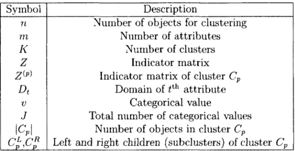
Symbol n m K Z Z(P)

A

\c

\

Number of objects for clustering Number of attributes

Number of clusters Indicator matrix Indicator matrix of cluster Cp

Domain of tth attribute

Categorical value

Total number of categorical values Number of objects in cluster Cp

Left and right children (subclusters) of cluster Cp

Table 2.2: Summary of notation used in Chapter 2 and 3

in order to create the indicator matrix, denoted by Z, which is a Boolean disjunctive table. Given the original categorical data set T, we denote the number of values for the tth categorical attribute by \Dt\. For each attribute At of the original categorical

data, there are \Dt\ corresponding columns. Therefore, there will be J = ]T)£Li IAI

columns in Z to represent all the original attributes. Here identical values from different attributes are treated as distinct. The indicator matrix Z is of order n x J, with each element defined as follows:

{

0, otherwise.

Here the jt h (1 < j < J) categorical value corresponds to the jt h column of Z. In the

remainder of this thesis, we use Z* to denote categorical object A', according to the indicator matrix data representation.

For each attribute, we expand its single original column to |Dt| columns, each

categorical value taking one column. Of the \Dt\ columns, only one column

corre-sponding to the categorical value takes the value 1, while the other columns take the value 0. So the sum of each row of matrix Z is in. This unified data presentation for categorical data also simplifies the following dissimilarity calculation. Furthermore, the role played by each categorical value in forming clusters can be distinguished by

giving them different weights, which can be easily implemented under our new data presentation.

In the example below, a simple data set is used as a scenario to illustrate how the original categorical data is transformed into an indicator matrix. In Table 2.3, there are six categorical objects with three attributes, whose domains are D\ = {a,b,c},

D2 = {a, b, c}, D3 = {a, b, c}, respectively. Table 2.4 illustrates the 9-column indicator

matrix of the data set in Table 2.3.

1 2 3 4 5 6 D l a a a b b c D2 a c a b b b D 3 a b b a c c

Table 2.3: Categorical data set scenario

1 2 3 4 5 6 D l a 1 1 1 0 0 0 b 0 0 0 1 1 0 c 0 0 0 0 0 1 D2 a 1 0 1 0 0 0 b 0 0 0 1 1 1 c 0 1 0 0 0 0 D 3 a 1 0 0 1 0 0 b 0 1 1 0 0 0 c 0 0 0 0 1 1 Table 2.4: Indicator matrix of Table 2.3

An indicator matrix is thus a kind of redundant data representation. For each At,

we expand its single-column representation corresponding to the original attribute to a |D4|-column representation where each column corresponds to one value of At. For

each object, only one of the \Dt\ columns corresponding to the categorical value takes

the value 1, while the other columns take the value 0. So the sum of each row of matrix Z is the number of original attributes, m. This unified data presentation for categorical data simplifies the subsequent dissimilarity calculation.

As a special case of categorical data, transactional data can also be transformed to an indicator matrix. Each item of a transaction is analogous to one categorical attribute which can take two values indicating inclusion or non-inclusion of the item. To build the indicator matrix, each such attribute is then transformed to two columns, one corresponding to inclusion and the other to non-inclusion of the item. This is called a symmetric transformation. Thus, if we suppose there are a total of d items in the transaction data base, the indicator matrix of the transaction data will have

2d columns rather than d columns (asymmetric transformation of transaction data

results in a binary table with d columns). As the result of this transformation, each row of the indicator matrix is guaranteed to have the same sum value, which is d. For example, a transaction {a, c, d} over the full item set {a, b, c,d,e} is transformed to a row of its indicator matrix with ten columns: the row is [1, 0, 0, 1, 1, 0, 1, 0, 0, 1].

We exploit the standard approach [39] to MCA, i.e., applying a simple CA to the indicator matrix Z. Since Z has a total sum of nm, which is the total number of occurrences of all the categorical values, the correspondence matrix is P = Z/nm. Thus the vector of row mass of the correspondence matrix is r = ( l / n ) l , the row mass matrix is Dr = (l/n)I; the column mass matrix is Dc = (l/nm)diag(ZTZ), the

vector of column mass of the correspondence matrix can be written as c = Dc x 1.

Under the null hypothesis of independence [39], the expected value of pt] is rtc3, and

the difference between the observation and the expectation, called the residual value, is ptJ — rxCj. Normalization of the residual value involves dividing the difference by

the square root of rtcr So the standardized residuals matrix is written in matrix

notation as:

S = D-W (P - re*) D-W = v ^ ( ^ - ^ 1 1TDC) D-CV\ (2.1)

Hence, the singular value decomposition (SVD) to compute the residuals matrix (2.1) is as follows:

v ^ (— - - 1 1TDC^ D:1'2 = UHVr) (2.2)

\nm n J

where UTU = VTV = I. E is a diagonal matrix with singular values in descending

columns of U are called the left singular vectors, and those of V, the right singular vectors. The left singular vectors U give us the scale values for the n objects, while the right singular vectors V give us the scale values for the J categorical values. In CA, they are called principal coordinates of rows and principal coordinates of columns, denoted as follows:

Principal coordinates of rows:

Principal coordinates of columns:

F = D:1/2UE

G = D71/2VE

The principal coordinates of the rows and columns can be plotted in the same co-ordinate system, as shown in Section 2.6.1. This graphical representation, called a symmetric map, illustrates the pattern of association between rows and columns. To avoid numerical overflow caused by l/nm when n and m are very large values, the standardized residuals matrix (2.1) can be written in an equivalent form as:

S=(z- -11

D

J (mb

Y

, (2.3)

where Dc = dlay (ZTZ). The equivalent transformation also simplifies the

calcula-tion.

The MCA calculation on the residuals matrix (2.3) provides an effective way to measure the association among the objects. The sum of squared elements of the standardized residuals matrix, called total inertia in correspondence analysis, is as follows:

V ^ V % 2 _ V^ y ^ (zv ~ zj/n) _ 1 V^ V^ (zv ~ z-j/n) (2 4)

2-^Z^'v Z^Z^ mz mnZ^Z-j z in

% j i j j i j •"

where z 3 = ]T^ ztJ, ]T\ ~zjl *s *"ne Chi-square statistic measuring the association between each object Zt and the set of objects T from the perspective of correspondence

analysis, while from the perspective of clustering, it is a distance measure between Z, and T, i.e., the Chi-square distance dChi(Zi,T). Thus Formula (2.4) can be written

as follows:

E E 4 = ^ E ' W ^ , T ) . (

-

)

i j i

Thus the total inertia can be explained as the average of the Chi-square distances between objects and the data set. The total inertia can also be expressed in the following form:

s

E E 4 = trace(SiF) = traced) = £ a] (2.6)

i j i

From (2.5) and (2.6) we can see that the average of the Chi-square distances is equivalent to the sum of the eigenvalues from the MCA calculation. In MCA, an eigenvalue a2 represents the amount of inertia that reflects the relative importance of

the transformed dimension. The first dimension always explains the largest portion of the variance, and the second explains the largest portion of the remaining unexplained variance, etc. In divisive hierarchical clustering, the goal of splitting a cluster is to lower the variance within the resulting subclusters, which consists of lowering the average of the Chi-square distance, or equivalently, the sum of the eigenvalues from the MCA standpoint. We will further explain the relationship between MCA and clustering categorical data in Section 2.6.1.

2.5 Optimization perspective for clustering

cate-gorical d a t a

In this section, we formalize the general problem of clustering n categorical objects into K groups, which is defined in Section 2.3, from an optimization perspective. We propose an objective function, and calculate the cluster center by optimizing the objective function.

define the objective function. We argued previously that in some situations, the similarity defined between a single object and a set of objects is more meaningful than pairwise similarity, especially when there is no significant comparison that can be used to define pairwise similarity in cluster analysis [7, 88], as in the example given in Section 2.1. Furthermore, MCA calculation on the indicator matrix involves a measure of the Chi-square dissimilarity between a single object and a set of objects, so we set the objective of clustering categorical data set T into K groups so as to minimize the following objective function, i.e., the sum of Chi-square error (SCE):

K

SCE^Y. Y,

ch

(Z

,C

), (2.7)

where dch%{Zi- Ck) is the Chi-square distance between object Z, and cluster Ck, which

is defined as follows:

dCht(Z>,Ck) = T{zWk>)2. (2.8)

Here /J,kj(l < J < J) is the jt h element of the cluster center of cluster Ck, and object

Zz is in cluster Ck.

The cluster center can be determined by optimizing the objective function (2.7), from which, the cluster center of cluster Ck in (2.8) is defined as the square root of

the frequency of the categorical value in the cluster, i.e.,

Hkj = ^p{v3\Ck) = (jg-^ , (2.9)

where v3 is the jt h categorical value, z3 = Ylztec zv ^ 1S w o rt h noting that when

fikj = 0, {zXJ — (ikj) must be zero as ztJ must be zero: in this case, (ztJ — fikj) /(ikj =

0. We give the derivation below. It shows how the cluster center defined in (2.9) can be mathematically derived when the distance measure is defined as in (2.8) and the objective is to minimize the SCE defined in (2.7).

Specifically, the SCE function is written as

fc=i zteck j = i LLkj

We solve for the tth element of pt h cluster center //pf(l < t < J) which minimizes

equation (2.10) by differentiating the SCE, setting it equal to 0. The derivation is as follows:

-^—SCE = d y y y (^j - ^k3) Ofht OHvt t[ *£k ^ / %

= ST^ ST" V ^ d (ZIJ ~ A*fcj)

z^cP h d ^ ^

Under the hypothesis of independence of the dimensions (the same as the null hy-pothesis of independence in MCA), we get

d cnip - ST d {zit~Vpt?

dfipt fipt

2 (A*P« — zlt) fJ-pt — {l-ipt ~ ztt)

0

SCE= y

oupt ££, ofipt fipt

Zt€Cp ^ z,ecp V ; V Z2

J : ( I 4 ) . . ^ . I ^ ^ . ( I E < )

As zlt is a Boolean variable having value 0 or 1, z\t = zlt , npt= \ T^-J ^2Zl€C z*t)

Thus, the prototype of the cluster in categorical data is represented by the square root of the mean of the indicator matrix of the cluster.

2.6 The D H C C algorithm

A detailed description of DHCC is given in this section. In contrast to the agglomera-tive approach, DHCC starts with an all-inclusive cluster containing all the categorical objects, and repeatedly chooses one cluster to split into two subclusters. A binary tree is employed to represent the hierarchical structure of the clustering results, in a way similar to that used in conventional hierarchical clustering algorithms [26, 95]. Additionally, in this section, we explain why DHCC can discover clusters embedded in subspaces.

In DHCC, splitting a cluster Cp involves finding a suboptimal (if not optimal)

so-lution to the optimization problem on the data set Cp with A'=2. The overall scheme

of DHCC is given in the algorithm in Figure 2.1. The core of the DHCC algorithm is the bisection procedure, which consists of two phases, preliminary splitting (step 3) and refinement (step 4). The algorithm iteratively chooses a leaf cluster to split, unless no leaf cluster can be split to further improve clustering quality. The quality measure will be presented in Section 2.6.3.

Algorithm: Scheme of DHCC

1. Transform the original categorical data into indicator matrix Z. 2. Initialize a binary tree with a single root holding all the objects. 3. Choose one leaf cluster Cp to split into two clusters C^ and CJ?

based on MCA calculation on the indicator matrix Z^p\

4. Iteratively refine the objects in clusters C^ and Cp.

5. Repeat steps (3) and (4) until no leaf cluster can be split to improve the clustering quality.

2.6.1 Preliminary splitting

In each bisection step, we initialize the splitting based on MCA. From formulas (2.5) and (2.6) we can see that minimizing the objective function (2.7) in a bisection in-volves maximally decreasing the total inertia of the standardized residuals matrices of the two resulting subclusters. As the first dimension of the transformed space based on MCA accounts for the largest proportion of the total inertia, splitting a cluster based on the first dimension can efficiently generate a preliminary bisection toward the optimization of the objective function.

Preliminary splitting is performed as follows. To bisect cluster Cp with \CP\

ob-jects, we apply MCA on the indicator matrix Z^ of order \CP\ x J from the \CP\

objects to get the principal coordinates of rows, i.e., F( p\ The object Zx whose first

coordinate F8\p) < 0 (or [74l < 0) goes to the left child of Cp, which is denoted by

Cp. and the object Zt whose first coordinate Ftj > 0 (or U^ > 0) goes to the right

child of Cp, which is denoted by Cp. In this phase, MCA plays an important role in

analyzing the data globally, and the variance and data distribution of the objects are thus taken into account in the preliminary bisection.

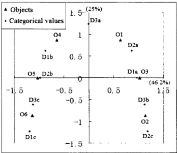
Why do we use only one dimension of the transformed space based on MCA to perform the preliminary bisection? Apart from the computational efficiency consider-ation, our concern is that other (less significant) dimensions may account for variance that is unlikely to be of interest in clustering, especially for the dimensions of lower inertia. Inappropriate involvement of these dimensions may result in adverse pre-liminary splitting. Take the data for the scenario in Table 2.3 for example. Clearly, the first 3 objects should be grouped together, as they are associated by the first attribute, having the common value 'a'; and the last 3 objects should likewise be grouped together, as they are associated by the second attribute, having the common value 'b'. The variance for the third attribute should be discarded in the clustering analysis. The symmetric map of the scenario data is given in Figure 2.2. The x-axis accounts for 46.2% of the total inertia, and the two clusters can be separated cor-rectly on this dimension. The categorical value 'a' on the third attribute has a large value on the y-axis, which accounts for 25% of the total inertia; however, it does not contribute to distinguish the two clusters as it appears once in both clusters. Division

according to the most significant dimension is very simple. It will be shown in our experiment that the simple preliminary division works well for clustering categorical data in DHCC. A Objects • Categorical values -1 0 4 it i. 5 -( 2 5 % ) 1 « Dlb 0. 5 0 5 D2b i« o . 5 -0. 5 D3c - o . 5 • CKS * -1 Die D3a -- 1 . 5 L -Ol 0.5 „ „ 1 D2a | • ' Dla 0 3 (46 2%t 1.J5 D3b j • A 0 2 D*2c ~ "

Figure 2.2: Symmetric correspondence analysis map of scenario data

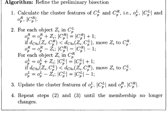
2.6.2 Refinement

The refinement phase attempts to improve the quality of the bisection by relocating the objects from the cluster being split. After the preliminary bisection, for each object from the parent cluster Cp, the refinement phase tries to improve the splitting

quality by finding which subcluster, Cp or Cp, is more suitable.

For computational efficiency, some cluster features associated with each cluster Cp

are maintained. One such feature is the J-dimensional vector of occurrence numbers of all the categorical values, denoted as op; the other is the number of objects in the

cluster, i.e., \CP\. Each element of op, conveniently represented here by z 3, is the

occurrence number of the jt h categorical value. The jt h element of cluster center can

be calculated as /J.P3 = \/z3/\Cp\, which in turn can be used to calculate the

Chi-square distance if the object Zt is in cluster Cp. If Zt is not in Cp, then the center