LH*
RS– A Highly-Available Scalable Distributed
Data Structure
WITOLD LITWIN U. Paris Dauphine and Rim Moussa U. Paris Dauphine andThomas J.E. Schwarz, S.J., Santa Clara University
________________________________________________________________________ LH*RS is a high-availability scalable distributed data structure (SDDS). An LH*RS file is hash partitioned over the distributed RAM of a multicomputer, e.g., a network of PCs, and supports the unavailability of any of its
k ≥ 1 server nodes. The value of k transparently grows with the file to offset the reliability decline. Only the number of the storage nodes potentially limits the file growth. The high-availability management uses a novel parity calculus that we have developed, based on the Reed-Salomon erasure correcting coding. The resulting parity storage overhead is about the minimal ever possible. The parity encoding and decoding are faster than for any other candidate coding we are aware of. We present our scheme and its performance analysis, including experiments with a prototype implementation on Wintel PCs. The capabilities of LH*RS offer new perspectives to data intensive applications, including the emerging ones of grids and of P2P computing.
Categories and Subject Descriptors: E.1 Distributed data structures, D.4.3 Distributed file systems, D.4.5 Reliability: Fault-tolerance, H.2.2 Physical Design : Access methods, Recovery and restart
General Terms: Scalable Distributed Data Structure, Linear Hashing, High-Availability, Physical Database Design, P2P, Grid Computing
________________________________________________________________________ Motto : Here is Edward Bear, coming downstairs now, bump, bump, bump, on the back of his head, behind Christopher Robin. It is, as far as he knows, the only way of coming downstairs, but sometimes he feels that there really is another way, if only he could stop bumping for a moment and think of it. And then he feels that perhaps there isn't. Winnie-the-Pooh. By A. A. Milne, with decorations by E. H. Shepard. Methuen & Co,
London (publ.)
1 INTRODUCTION
Shared–nothing configurations of computers connected by a high-speed link, often called
multicomputers, allow for high aggregate performance. These systems gain in popularity
with the emergence of grid computing and P2P applications. They need new data structures that scale with the number of components [CACM97]. The concept of a Scalable Distributed Data Structures (SDDS) aims at this goal [LNS93]. An SDDS file transparently scales over multiple nodes, called the SDDS servers. As the file grows, so does the number of servers on which it resides. The SDDS addressing scheme has no centralized components. The speed of operations is then possibly independent of the file size. Many SDDS schemes are now known. They provide for hash, range or m-d
Authors' addresses: Witold Litwin, Rim Moussa,Université Paris 9 (Dauphine), Pl. du Mal. de Lattre, Paris 75016, France, [email protected], [email protected]; Thomas J.E. Schwarz, S.J., Department of Computer Engineering, Santa Clara University, Santa Clara, mailto:[email protected]. Authors' addresses: Witold Litwin, Rim Moussa,Université Paris 9 (Dauphine), Pl. du Mal. de Lattre, Paris 75016, France, [email protected], [email protected]; Thomas J.E. Schwarz, S.J., Department of Computer Engineering, Santa Clara University, Santa Clara, mailto:[email protected]. Authors' addresses: Witold Litwin, Rim Moussa,Université Paris 9 (Dauphine), Pl. du Mal. de Lattre, Paris 75016, France, [email protected], [email protected]; Thomas J.E. Schwarz, S.J., Department of Computer Engineering, Santa Clara University, Santa Clara, mailto:[email protected]. Authors' addresses: Witold Litwin, Rim Moussa,Université Paris 9 (Dauphine), Pl. du Mal. de Lattre, Paris 75016, France, [email protected], [email protected]; Thomas J.E. Schwarz, S.J., Department of Computer Engineering, Santa Clara University, Santa Clara, mailto:[email protected].
partitioned files of records identified with a primary or with multiple keys. See [SDDS] for a partial list of references. A prototype system, SDDS 2000, for Wintel PCs, is freely available for a non-commercial purpose [CERIA].
Among best-known SDDS schemes is the LH* scheme [LNS93, LNS96, KLR96, BVW96, B99a, K98v3, R98]. It creates scalable distributed hash partitioned files. Each server stores the records in a bucket. The buckets split when the file scales up. The splits follow the linear hashing (LH) principles [L80a, L80b]. Buckets are usually stored in distributed RAM. Only the maximum number of nodes of the multicomputer limits the file size. A search or an insert of a record in an LH* file can be hundreds times faster than a disk access [BDNL00, B02].
An LH* server may become unavailable (failed), which makes it impossible to access its data. The likelihood of a server unavailability increases with the scaling file. Similarly, the likelihood of k unavailable servers for any fixed k increases with file size. Data loss or inaccessibility can be very costly [CRP06]. The well-known crash of EBay in June 1999 resulted in a loss of $4B of market value and of $25M in operations. The failure of a financial database may easily cost $10K-$27K per minute, [B99].
The information-theoretical minimum storage overhead for k-availability of m data servers is k/m [H&al94]. It requires the encoding of k parity symbols (records, buckets…), per m data symbols (records, buckets…). Decoding k unavailable symbols requires access to m available symbols among m + k. Large values for m seem impractical. One approach to reasonably limit m is to partition a data file into groups with independent parity calculus, of m nodes (buckets) at most per group.
For a small file using a few servers, a failure of more than one node is unlikely. Thus,
k = 1 availability should typically suffice. The parity overhead is then the smallest, 1/m,
and the parity operations the fastest, using only XORing, as in RAID-5. The probability that a server becomes unavailable increases however with the size of the file. We need availability levels of k > 1 despite the increased storage overhead. Any static choice for k becomes eventually too small. The probability that k servers become unavailable increases necessarily. The file reliability, which is the probability that all the data are available for the application, declines necessarily as well. To offset this decline, we need the scalable availability, making k dynamically growing with the file [LMR98].
Below, we present an efficient scalable availability scheme we called LH*RS. It generalizes the LH* scheme, structuring the scaling data file into groups of m data buckets, as we indicated above. The parity calculus uses a novel variant of Reed-Solomon (RS) erasure correcting coding/decoding we have designed. To our best
knowledge, it offers the fastest encoding for our needs. The storage overhead remains in particular in practice about optimal, between k/m and (k+1)/m.
We recall that RS codes use a parity matrix in a Galois Field (GF), typically in a
GF (2f
). The GF (216) turned out to be the most efficient for us at present. The addition in a GF is fast, amounting to XORing. The multiplication is slower, regardless of the algorithm used [MS97]. Our parity calculus for k = 1 applies the XORing only, optimizing the most common case. We resort to GF multiplication only for k > 1. Our multiplication uses log and antilog tables. One novelty is that the XORing only encoding remains however then for the first parity symbol (record, bucket…), and for the decoding of a single unavailability of a data bucket. Another novelty is an additional acceleration of the encoding, by needing only XOR operations for the first bucket in each bucket group. Finally, we innovate by using a logarithmic parity matrix, as we will explain, accelerating the parity calculus even more. Besides, the high-availability management does not affect the speed of searches and scans. These operations perform as in an LH* file with the same data records and bucket size.
The study of LH*RS we present here stems from our initial proposals in [LS00]. The analysis reported below has perfected the scheme. This includes various improvements to the parity calculus, such as the use of GF(216) instead GF(28), as well as more extensive use of XORing and of the logarithmic parity matrices. We will show other aspects of the evolution in what follows. We have also completed the study of various operational aspects of the scheme, especially of messaging, crucial for the performance.
LH*RS is the only high-availability SDDS scheme operational to the extend we present, demonstrated by a prototype for Wintel PCs, [LMS04]. It is not however the only one known. There were proposals to use the mirroring for to achieve 1-availability [LN96, BV98, VBW98]. Two schemes using only XORing provide 1-availability [L&al97, LR01, L97]. Another XORing-only scheme LH*SA was the first to offer the scalable availability [LMRS99]. Its encoding speed can be faster than for LH*RS. The price is sometimes greater storage overhead. We compare various schemes in the related work section.
We first describe the general structure of an LH*RS file and the addressing rules. Next, we discuss the mathematics of the parity calculus and its use for the LH*RS encoding and decoding. We then present the basic LH*RS file manipulations. We follow with a theoretical and experimental performance analysis of the prototype. Our measurements justify various design choices for the basic scheme and confirm its promising efficiency. In one of our experiments, about 1.5 sec sufficed to recover 100 000 records in three
unavailable data buckets, with more than 10MB of data. We investigate also variants with different trade-offs, including a different choice of an erasure correcting code. Finally we discuss the related work, the conclusions and the directions for future work. The capabilities of LH*RS appear to open new perspectives for data intensive applications, including the emerging applications of grids and of P2P computing.
Section 2 describes the LH*RS file structure. Section 3 presents the parity encoding. Section 4 discusses the data decoding. We explain the LH*RS file manipulations in Section 5. Section 6 deals with the performance analysis. In Section 7 we investigates variants to the scheme. Section 8 discusses the related work. Section 9 concludes the study and proposes directions for the future work. Appendix A shows our parity matrices for GF (216) and GF (28). Appendix B sums up our terminology.
2 THE LH*RS FILE STRUCTURE
LH*RS provides high availability to the LH* scheme [LNS93, LNS96, LMRS99]. LH* itself is the scalable distributed generalization of Linear Hashing (LH) [L80a, L80b]. An LH*RS file contains data records and parity records. Data records contain the application data. The application interacts with the data records as in an LH* file. Parity records provide high availability and are invisible to the application.
We store the data and parity records at the server nodes of the LH*RS file. The application does not access the servers directly, but uses the services of the LH*RS client component. A client usually resides at the application node. It acts as a middleware between the application and the servers.
An LH*RS operation is in normal mode as long as it does not access an unavailable bucket. If it does, the operation enters degraded mode. In what follows, we assume normal mode unless otherwise stated. We first present the storage and addressing of the data records. We introduce the parity management afterwards.
2.1 Data Records
2.1.1 Storage
An LH*RS file stores data records as if they constituted an LH*LH file, a variant of LH* described in [KLR96]. The details and correctness proofs of the algorithms presented below are in [KLR96] and [LNS96]. A data record consists of a (primary) key field, that identifies the record, and a non-key field, Figure 1. The application provides the data for both fields. We write c for the key. The records are stored in data buckets, numbered 0, 1, 2… and located each at a different server node of the multicomputer. The location of bucket a, i.e., the actual address A of the node supporting it, results from a mapping
[LNSb96]. A data bucket has the capacity to store b>>1 data records. Additional records become overflow records. Each bucket reports an overflow to the coordinator component of LH*. Typically, the coordinator resides at node of bucket 0.
Initially, an LH*RS file typically stores its data records only in bucket 0 at some server
A0. It also contains at least one parity bucket, at a different server, as we discuss later. The file adjusts to growth by dynamically increasing (or decreasing) the number of buckets. New buckets are created by splits. Inserts that overflow their buckets trigger these. Inversely, deletion causing an underflow may trigger bucket merges. Each merge undoes the last split, freeing the last bucket. The coordinator manages both splits and merges.
We show now how LH*RS data buckets split in normal mode. In Section 5, we treat the processing of the parity records during the splits, as well the degraded mode. We postpone the description of the merge operation to that section too.
As in LH file, the LH*RS buckets split in fixed order: 0; 0,1; 0,1,2,3; …; 0…n,…2i -1; 0… The coordinator maintains the data (i, n) forming the file state. The variable i determines the hash function used to address the data records, as we discuss in Section 2.1.2 below. We call i the LH* file level. The variable n points to the bucket to split; we call it the split pointer. Initially, (i, n) = (0,0).
To trigger a split, the coordinator sends a split message to bucket n. It also dynamically appends a new bucket to the file with the address n + 2i. The address of each key c in bucket n is then recalculated using a hash function hi+1: c → c mod 2i+1. We call the functions hi linear hash functions (LH-function). For any record in bucket n, either hi+1 (c) = n or hi+1 (c) = n + 2i. Accordingly, any record either remains in bucket n or migrates to the new bucket n + 2i. Assuming as usual that key values are randomly distributed, both events are equally likely.
After the split, the coordinator updates n as follows. If n < 2i - 1, it increments n to
n + 1. Otherwise it sets it to n = 0 and increments i to i + 1.
Internally, each LH*RS data bucket a is organized as an LH file. We call the internal buckets pages. There is also an internal file state, called the bucket state, (ĩ, ñ). We perform the LH*RS split, (and the LH*LH split in general [KLR96]), by moving all odd pages to the new bucket a’. This is faster than the basic technique of recalculating the address for every record in bucket a. We rename the odd pages in the new bucket a’ to 0, 1… by dropping the least significant bit. Likewise, we rename the even pages in bucket a. In other words, page number p becomes page number p/2 in the new buckets.
We also decrement the level l of the pages by one. The internal file state in the new bucket a’ becomes (ĩ –1, ⎣ñ/2⎦ ). We change the file state of the splitting bucket to (ĩ, ñ) := (ĩ, 0) if ñ = 2ĩ – 1, and to (ĩ, ñ) := (ĩ –1, ⎣ñ+1⎦/2) otherwise. See [KLR96] for details. We deal with page merges accordingly.
2.1.2 Addressing
The LH* storage rules guarantee that for any given file state (i, n), the following LH
addressing algorithm [L80a] determines the bucket a for a data record with key c
uniquely:
(A1) a := hi (c); if a < n then a := hi + 1 (c).
Algorithm (A1) determines the correct (primary) address for key c. Its calculus depends on the file state at the coordinator. The general principles of SDDS mandate avoiding hot spots. Therefore, LH*RS clients do not access the coordinator to obtain the file state. Each client uses instead (A1) on its private copy of the file state. We call it
client image, and write as (i’,n’). Initially, for a new client or file, (i', n') = (0,0), as the
initial file state. In general, the client image differs from the file state, as the coordinator does not notify the clients of any bucket splits and merges. The strategy reflects the basic SDDS design, avoiding excessive messaging after a split, problems with unavailable clients, etc. [LNS96]. As the result, any split or merge causes all client images to be out of date.
Using (A1) on the client image can lead to an incorrect address. The client then sends the request to an incorrect bucket. The receiving bucket forwards the request that normally reaches the correct server in one or at most two additional hops (as we will show more below). The correct LH*RS server sends an image adjustment message (IAM). The IAM adjusts the image so that the same addressing error cannot occur again. It does not guarantee that the image becomes equal to the file state. In general, different clients may have different images.
The binding between bucket numbers and node addresses is done locally as well. Buckets can change their location. For instance, a bucket can merge with its “father” bucket, and then again split off, but on another (spare) server. A bucket located on a failed node is also reconstructed on a spare. We call a bucket, and query to it, displaced if the bucket is located at a different server than the client knows. We use IAM message to update these data whenever the client deals with a displaced bucket. It will appear that the presence of displaced bucket may lead to one or two additional hops.
returns all records satisfying a certain condition. We treat scans in Section 5.5. The key-based operations are insert, delete, update, and (key) search. To perform such an operation, the client uses (A1) to obtain a bucket address a1 and sends the operation to this bucket. Most of the time [LNS96], the correct bucket number ã, is identical to a1. However, if the file grew and now contains more buckets, then a1 < ã is possible. If the file shrank, then a1 > a is possible as well. In both cases, the client image differed from the file image.
To be able to resolve the incorrectly addressed operations, every bucket stores the j value of hj last used to split or to create the bucket. We call j the bucket level and we have
j = i or j = i + 1. A server that receives a message intended for bucket ã, first tests
whether it really has bucket ã. If not, it forwards the displaced query to the coordinator. The coordinator attempts to resolve the addressing using the file state. We treat this case later in this section.
Otherwise, bucket ã starts the LH* forwarding algorithm (A2): (A2) a' := hj (c) ;
if a' = ã then accept c ; else a'' := hj - 1 (c) ;
if a'' > ã and a'' < a' then a' := a'' ;
send c to bucket a' ;If the address a' provided by (A2) is not ã, then the client image was incorrect. Then, bucket ã forwards the query to bucket a2 = a', a2 > a1. If the query is not displaced, bucket a2 becomes the new intended bucket for the query, i.e.,
ã := a2. It acts accordingly, i.e., executes (A2). This may result in the query forwarded to yet another bucket a3 := a', with a' recalculated at bucket a2 and a3 > a2. Bucket a3 becomes the next intended bucket, i.e., ã := a3. If the query is not displaced, bucket a3 acts accordingly in turn, i.e., it executes (A2). A basic property of LH* scheme is then that (A2) must yield a' = a3, i.e., bucket a3 must be the correct bucket a. In other words, the scheme forwards a key-based operation at most twice.
The correct bucket a performs the operation. In addition, if it received the operation through forwarding i.e. a ≠ a1, it sends an IAM to the client. The IAM contains the level
j of bucket a1 (as well as the locations known to bucket a, which are in fact all those of its preceding buckets). The client uses the IAM to update its image as follows, according to the LH* Image Adjustment algorithm:
(A3) if j > i' then i' := j - 1, n' := a +1 ; if n' ≥ 2i' then n' = 0, i' := i' +1 ;
(A3) guarantees that the client cannot repeat the same error, although the client image typically still differs from the file image. The client also updates its location data.
We process the query within the correct bucket as a normal LH query. We locate first the page that contains the key c. However, if the bucket has level j > 0, we do not apply the addressing algorithm (A1) directly to c, but rather to c shifted by j bits to the right. In other words, we apply (A1) to ⎣c/2j⎦. The modification corresponds to the algorithm for splitting buckets described in the previous section, [KLR96].
If a server forwards a displaced query to the coordinator, the latter calculates the correct address a. It does so according to (A1) and the file state. It sends the actual location of the displaced bucket to the query originator and to the server. These update their locations accordingly.
2.2 Parity Records
The LH*RS parity records protect an application against the unavailability of servers with its stored data. The LH*RS file tolerates up to k ≥ 1 unavailable server in a manner transparent to the application. As usual, we call this property k-availability. The (actual)
availability level k depends on an LH*RS file specific parameter, the intended availability
level K ≥ 1. We adjust K dynamically with the size of the file, (Section 2.2.3). Depending on the file state, the actual availability level k is either K or K–1.
2.2.1 Record Grouping
LH*RS parity records constitute a specific structure, invisible to the application, and separate from the LH* structure of the data records. The structure consists of bucket
groups and record groups. We collect all buckets a with
⎢
⎣
a m/⎥
⎦
=gin a bucket groupg, g = 0, 1 ... Here, m > 0 is a file parameter that is a power of 2. In practice, we only
consider m ≤ 128, as we do not envision currently any applications where a larger value might be practical. A bucket group consists thus of m consecutively numbered buckets, except perhaps for the last bucket group with less than m members.
Data records in a bucket group form record groups. Each record group (g,r) is identified by a unique rank r, and the bucket group number g. At most one record in a bucket has any given rank r. The record gets its rank, when an insert or split operation places it into the bucket. Essentially, records arriving at a bucket are given successive ranks, i.e. r = 1, 2… However, we can reuse ranks of deleted records. A record group contains up to m data records, each at a different bucket in the bucket group. A record that moves with a split obtains a new rank in the new bucket. For example, the first record arriving at a bucket a, a = 0, 1 ... m–1, because of an insert or a split, obtains rank 1. It thus joins the record group (0,1). If the record is not deleted, before the next record arrives at that bucket, that one joins group (0,2), etc.
Each record group has k ≥ 1 parity records p1 … pk in addition to the data records. The parity records are stored at different parity buckets P1, ... Pk. The local availability
level k depends on the intended availability level K, the bucket group number g, and the
file state. Using the parity calculus presented in Section 3 and given any s ≤ k parity records and any m-s data records, we can recover the remaining l data records in the group. The availability level of the file is the minimum of the local availability levels.
2.2.2 Record Structure
Figure 1 (ii) shows the structure of a parity record for group (g,r). The first field of every record pi of the group contains the rank r as the record key in Pi. The next field is the (record) group structure field C = c0, c1, … cm-1. If there is a data record in the ith bucket of the group, then ci is the key of that data record. Otherwise, ci is zero.
The final field is the parity field B. The contents of B are the parity symbols. We calculate them from the non-key data in the data records in the record group (Section 3) in a process called encoding. Inversely, given s parity fields and m-s non-key data fields from records in the group, we can recover the remaining non-key data fields using the
decoding process from Section 3. We can recover the keys of the s lacking data records
from any parity record.
Figure 1: LH*RS record structure: (i) data record, (ii) parity record.
In [LS00], we used a variable length list of keys for existing data structures. The fixed structure presented here and introduced since in [Lj00], proved however more efficient. It typically needs slightly less storage. In addition, its position indicates the bucket at which data records are located. During record recovery, we can directly access the bucket instead of using the LH* addressing algorithm. We avoid possible forwarding messages.
2.2.3 Scalable Availability
Storing and maintaining parity creates storage overhead increasing with k. For a file with only 1 data bucket, the overhead is k. For a larger file, the overhead is at least equal to
k/m. In addition, we have the run-time overhead to update all k parity records of a group
whenever the application inserts, updates or deletes a data record. A file with few buckets is less likely to suffer from multiple unavailable buckets. However, as the size of the file increases, multiple failures become more probable. For any given k, the probability of catastrophic loss, i.e. loss of more than k buckets in a single group and the resulting inability to access all records, increases with the file size [H&a94]. In response,
c non-key data r c0, c1, c2 B
the LH*RS scheme provides the scalable availability, [LMR98]. When the growing file reaches certain sizes, the file starts to incrementally increase every local k-availability to
k+1-availability. We illustrate the principle in Figure 2 that we will discuss more in depth
soon.
Specifically, we maintain the file parameter termed intended availability level K. If we create a new bucket that is the first in the group, then this group gets k = K parity buckets. Every data record in this group has then k = K parity records. Initially, K = 1, and any group has one parity bucket. We basically increment K when (i) the split pointer returns to bucket 0, and (ii) the total number of buckets reaches some predetermined level. Then, any existing bucket group has k = K – 1 parity buckets (as we will see by induction). Every new group gets then K parity buckets. In addition, whenever we split the first bucket in a group, we equip this group with an additional parity bucket. As the split pointer moves through the data buckets of the file, we create all new groups with K parity buckets, and add an additional parity bucket to all old groups. Thus, by the time the split pointer reaches bucket 0 again, all groups have local availability level k = K.
In Figure 2, a bucket group has the size of m = 4. Data buckets are white and parity buckets are grey. In Figure 2a, we create the file with one data bucket and one parity bucket, i.e., with K = 1. When the file size increases, we split the first bucket, but only maintain one parity bucket, Figure 2b,c. When the m+1st bucket is created, the new bucket group receives also receives a parity bucket. Thus, the file is 1-available. Each new bucket group has this availability level until the number N of data buckets in the file reaches some N1. In our example, N1 = 16, Figure 2e. More generally, N1 = 2l with some large l >> 1 in practice. That condition implies n = 0. The next bucket to split is bucket 0.
At this point of the file scale up, K increases by one. From now on, starting with the split of bucket 0, each split creates two parity records per record group, Figure 2f. Both the existing group and the one started by the split have 2 parity buckets. The process continues until some size N2, also a power of 2 and, necessarily this time, a multiple of m. On the way, starting from the file size N = 2N1, all the bucket groups are 2-available, Figure 2g. When the file grows to include N2 buckets, K increases by 1 again, to K = 3 this time. The next split adds a third parity bucket to the group of bucket 0 and initializes a new group starting with bucket N2 and carrying three parity buckets. The next series of splits provides all groups with K = 3 parity records. When the file size reaches N3, K is again incremented, etc.
Ni+1 =2 i N1. We call this strategy uncontrolled availability and justify it in [LMR98]. Alternatively, a controlled availability strategy implies that the coordinator calculates dynamically the values of the Ni. The decision may be based on the probability of k unavailable buckets in a bucket group, whenever the split pointer n comes back to 0.
(a) (b) (c)
(d) (e)
(f)
(g)
(h)
…
Figure 2: Scalable Availability of LH*RS File.
The global file availability level Kfile is the maximum k so that we can recover any k buckets failing simultaneously. Obviously, Kfile is equal to the minimum k for all groups in the file. We thus have Kfile = K or Kfile = K–1. Kfile starts at 1 and increases to Kfile = 2, when N reaches 2N1. In general, K increases to i after N reaches Ni and Kfile reaches i when N reaches 2Ni. The growing LH*RS file is thus progressively able to recover from larger and larger numbers of unavailable buckets, as these events become increasingly likely, necessarily.
One consequence of the scheme is the possible presence of transitional bucket groups where not all the data buckets are split yet. The split pointer n points there somewhere between the 2nd and the last bucket of the group. The first bucket group in Figure 2f is transitional, as well as in Figure 2h, both with n = 2. In such a group, the newly added parity bucket only encodes the contents of the data buckets that have already split. LH*RS recovery cannot use this additional parity bucket in conjunction with data buckets that have not yet split. As the result, the availability level of any transitional group is K – 1. It becomes K when the last bucket splits, (hence the group ceases to be transitional).
3 PARITY ENCODING
record. Section 4 deals with the decoding for the reconstruction of an unavailable record. The parity encoding in general is based on Erasure Correcting Codes (ECC). We have designed a generalization of a Reed-Solomon (RS) code. RS codes are popular, [MS97], [P97], being sometimes indirectly referred to also as information dispersal codes, [R89]. Other codes are a possibility, we discuss the trade-offs in Section 7.5. Our parity calculations are operations in a Galois Field (GF) as detailed in Section 3.1. We use a
parity matrix (Section 3.2), which is a submatrix of a generator matrix (Section 4.1).
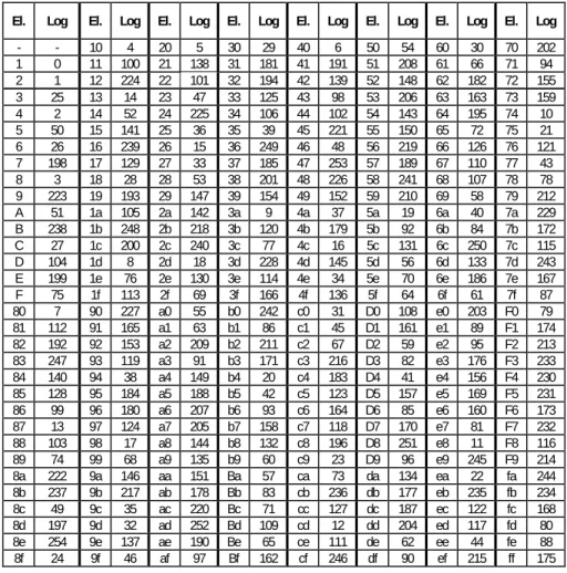
El. Log El. Log El. Log El. Log El. Log El. Log El. Log El. Log - - 10 4 20 5 30 29 40 6 50 54 60 30 70 202 1 0 11 100 21 138 31 181 41 191 51 208 61 66 71 94 2 1 12 224 22 101 32 194 42 139 52 148 62 182 72 155 3 25 13 14 23 47 33 125 43 98 53 206 63 163 73 159 4 2 14 52 24 225 34 106 44 102 54 143 64 195 74 10 5 50 15 141 25 36 35 39 45 221 55 150 65 72 75 21 6 26 16 239 26 15 36 249 46 48 56 219 66 126 76 121 7 198 17 129 27 33 37 185 47 253 57 189 67 110 77 43 8 3 18 28 28 53 38 201 48 226 58 241 68 107 78 78 9 223 19 193 29 147 39 154 49 152 59 210 69 58 79 212 A 51 1a 105 2a 142 3a 9 4a 37 5a 19 6a 40 7a 229 B 238 1b 248 2b 218 3b 120 4b 179 5b 92 6b 84 7b 172 C 27 1c 200 2c 240 3c 77 4c 16 5c 131 6c 250 7c 115 D 104 1d 8 2d 18 3d 228 4d 145 5d 56 6d 133 7d 243 E 199 1e 76 2e 130 3e 114 4e 34 5e 70 6e 186 7e 167 F 75 1f 113 2f 69 3f 166 4f 136 5f 64 6f 61 7f 87 80 7 90 227 a0 55 b0 242 c0 31 D0 108 e0 203 F0 79 81 112 91 165 a1 63 b1 86 c1 45 D1 161 e1 89 F1 174 82 192 92 153 a2 209 b2 211 c2 67 D2 59 e2 95 F2 213 83 247 93 119 a3 91 b3 171 c3 216 D3 82 e3 176 F3 233 84 140 94 38 a4 149 b4 20 c4 183 D4 41 e4 156 F4 230 85 128 95 184 a5 188 b5 42 c5 123 D5 157 e5 169 F5 231 86 99 96 180 a6 207 b6 93 c6 164 D6 85 e6 160 F6 173 87 13 97 124 a7 205 b7 158 c7 118 D7 170 e7 81 F7 232 88 103 98 17 a8 144 b8 132 c8 196 D8 251 e8 11 F8 116 89 74 99 68 a9 135 b9 60 c9 23 D9 96 e9 245 F9 214 8a 222 9a 146 aa 151 Ba 57 ca 73 da 134 ea 22 fa 244 8b 237 9b 217 ab 178 Bb 83 cb 236 db 177 eb 235 fb 234 8c 49 9c 35 ac 220 Bc 71 cc 127 dc 187 ec 122 fc 168 8d 197 9d 32 ad 252 Bd 109 cd 12 dd 204 ed 117 fd 80 8e 254 9e 137 ae 190 Be 65 ce 111 de 62 ee 44 fe 88 8f 24 9f 46 af 97 Bf 162 cf 246 df 90 ef 215 ff 175
Table 1: Logarithms for GF(256). 3.1 Galois Field
Our GF has 2f elements ; f = 1,2…, called symbols. Whenever the size 2f of a GF matters, we note the field as GF(2f). Each symbol in GF(2f) is a bit-string of length f. One symbol is zero, written as 0, consisting of f zero-bits. Another is the one symbol, written as 1, with f-1 bits 0 followed by bit 1. Symbols can be added (+), multiplied (⋅), subtracted (-) and divided (/). These operations in a GF possess the usual properties of their analogues
in the field of real or complex numbers, including the properties of 0 and 1. As usual, we may omit the ‘⋅’ symbol.
Initially, we elaborated the LH*RS scheme for f = 4, [LS00]. First experiments showed that f = 8 was more efficient. The reason was the (8-bit) byte and word oriented structure of current computers [Lj00]. Later, the choice of f = 16 proved even more practical. It became our final choice, Section 6.3. For didactic purposes, we discuss our parity calculus nevertheless for f = 8, i.e., for GF(28) = GF(256). The reason is the sizes of the tables and matrices involved. We note this GF as F. The symbols of F are all the byte values. F has thus 256 symbols which are 0,1…255 in decimal notation, or 0,1...ff in hexadecimal notation. We use the latter in Table 1 and often in our examples.
The addition and the subtraction in any our GF(2f ) are the same. These are the bit-wise XOR (Exclusive-OR) operation on f-bit bytes or words. That is:
a + b = a – b = b – a = a ⊕ b = a XOR b.
The XOR operation is widely available, e.g., as the ^ operator in C and Java, i.e., a XOR
b = a ^ b. The multiplication and division are more complex operations. There are
different methods for their calculus. We use a variant of the log/antilog table calculus [LS00], [MS97].
GFElement mult (GFElement left,GFElement right) { if(left==0 || right==0) return 0;
return antilog[log[left]+log[right]]; }
Figure 3: Galois Field Multiplication Algorithm.
The calculus exploits the existence in every GF of the primitive elements. If α is primitive, then any element ξ ≠ 0 is αi for some integer power i, 0 ≤ i < 2f
– 1. We call i the logarithm of ξ and write i = logα(ξ). Table 1 tabulates the non-zero GF(28
) elements and their logarithms for α = 2. Likewise, ξ = αi
is then the antilogarithm of i that we write as ξ = antilog (i).
The successive powers αi for any i, including i ≥ 2f
– 1 form a cyclic group of order 2f – 1, with αi = αi’ exactly if i’ = i mod 2f–1. Using the logarithms and the antilogarithms, we can calculate multiplication and division through the following formulae. They apply to symbols ξ,ψ ≠ 0. If one of the symbols is 0, then the product is obviously 0. The addition and subtraction in the formulae is the usual one of integers:
ξ⋅ψ = antilog( log(ξ) + log(ψ) mod (2f –1)), ξ/ψ = antilog( log(ξ) – log(ψ) + 2f
To implement these formulae, we store symbols as char type (byte long) for GF(28) and as short integers (2-byte long) for GF(216). This way, we use them as offsets into arrays. We store the logarithms and antilogarithms in two arrays. The logarithm array log has 2f entries. Its offsets are symbols 0x00 … 0xff, and entry i contains log(i), an unsigned integer. Since element 0 has no logarithm, that entry is a dummy value such as 0xffffffff. Table 1 shows the logarithms for F.
Our multiplication algorithm applies the antilogarithm to sums of logarithms modulo 2f–1. To avoid the modulus calculation, we use all possible sums of logarithms as offsets. The resulting antilog array then stores antilog[i] = antilog( i mod (2f–1)) for entries i = 0, 1, 2…, 2(2f–2). We double the size of the antilog array in this way to avoid the modulus calculus for the multiplication. This speeds up both encoding and decoding times. We could similarly avoid the modulo operation for the division as well. In our scheme however, division are rare and the savings seem too minute to justify the additional storage (128KB for our final choice of f = 16). Figure 3 shows our final multiplication algorithm. Figure 4 shows the algorithm generating our two arrays. We call them respectively log and antilog arrays. The following example illustrates their use.
Example 1
We use the result of the following GF(28) calculation later in Example 2: 45 1 49 1a 41 3b 41 ff
45 antilog(log(49)+log(1a)) antilog(log(41)+log(3b)) antilog(log(41)+log(ff)) 45 + antilog(152 105) antilog(191 120) antilog(191+175)
45 + antilog(257) antilog(311) antilog(191+
⋅ + ⋅ + ⋅ + ⋅
= + + +
= + + + +
= + + 175)
45 antilog(2) antilog(56) antilog(111) 45 04 5d ce
d2
= + + +
= + + +
=
The first equality uses our multiplication formula but for the first term. We use the logarithm array log to look up the logarithms. For the second term, the logarithms of 49 and 1a are 152 and 105 (in decimal) respectively (Table 1). We add these up as integers to obtain 257. This value is not in Table 1, but antilog[257]=4, since logarithms repeat the cycle of mod (2f–1) that yields here 255. The last equation sums up four addends in the Galois field, which in binary are 0100 0101, 0000 0100, 0101 1101, and 1100 1110. Their sum is the XOR of these bit strings yielding here 1101 0010 = d2.
To illustrate the division, we calculate 1a / 49 in the same GF. The logarithm of 1a is 105, the logarithm of 49 is 152. The integer difference is –47. We add 255, obtain 208,
hence read antilog[208]. According to Table 1 it contains 51 (in hex), which is the final result.
3.2 Parity Matrix
3.2.1 Parity Calculus
We recall that a parity record contains the keys of the data records and the parity data of the non-key fields of the data records in a record group, Figure 1. We encode the parity data from the non-key data as follows.
We number the data records in the record group 0, 1,… m-1. We represent the non-key field of the data record j as a sequence
a
0,j,
a
1,j,
a
2,jK
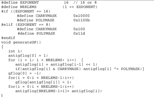
of symbols. We give to all the records in the group the same length l by at least formally padding with zero symbols if necessary. If the record group does not contain m records, then we (conceptually) replace the missing records with dummy records consisting of l zeroes.#define EXPONENT 16 // 16 or 8
#define NRELEMS (1 << EXPONENT) #if ((EXPONENT == 16) #define CARRYMASK 0x10000 #define POLYMASK 0x1100b #elif (EXPONENT == 8) #define CARRYMASK 0x100 #define POLYMASK 0x11d #endif void generateGF() { int i; antigflog[0] = 1;
for (i = 1; i < NRELEMS; i++) { antigflog[i] = antigflog[i-1] << 1;
if(antigflog[i] & CARRYMASK) antigflog[i] ^= POLYMASK;} gflog[0] = -1;
for(i = 0;i < NRELEMS-1;i++) gflog[antigflog[i]] = i; for(i = 0;i < NRELEMS-1;i++)
antigflog[NRELEMS-1+i]= antigflog[i]; }
Figure 4: Calculus of tables log and antilog for GF(2f).
We consider all the data records then in the group as the columns of an l by m matrixA=
( )
ai,j . We also number the parity records in the record group 0,1…k. Wewrite b0,j,b1,j,b2,j,K for the B-field symbols of the jth parity record. We arrange the parity records also in a matrix with l rows and k columnsB=
( )
bi,j . Finally, we considerthe parity matrix P= p
( )
λ µ, that is a matrix of symbols p forming m rows and k columns. We show the construction of P in next sections. Its key property is the linearrelationship between the non-key fields of data records in the group and the non-key fields of the parity records:
. B P
A⋅ =
More in depth, each jth row of A is a vector
a
j=
(
a
j,0,
a
j,1,
K
,
a
j m, −1)
of the symbols in all the successive data records with the same offset j. Likewise, every jth line b j of B contains the parity symbols with the same offset j in the successive parity records of the record group. The above relationship means that:b j = a j P.
Each parity symbol is thus the sum of m products of data symbols with the same offset times m coefficients of a column of the parity matrix:
(3.1) 1 , , , 0
.
m j j b λ a ν pν λ ν − = =∑
⋅The LH*RS parity calculus does not use P directly. Instead, we use the logarithmic
parity matrix Q with coefficients qi,j = logα(pi,j). The implementation of equation (3.1) gets the form:
(3.2) , 01antilog( , log( , ))
m
bι λ ν− qν λ aι ν
=
=
⊕
+Here,
⊕
designates XOR and the antilog designates the calculus using our antilog table, which avoids the mod (2f–1) computation. Using (3.2) and Q instead of (3.1) and P speeds up the encoding, by avoiding half of the accesses to the log table. The overall speed-up of the encoding is however more moderate than one could perhaps expect from these figures (Section 6.3.1). While using Q that is our actual approach, we continue to present the parity calculus in terms of P for ease of presentation.3.2.2 Generic Parity Matrices
We have designed for LH*RS several algorithms for generating parity matrices. We presented the first one in [LS00] for 4-bit symbols of GF(24). When implemented, operations turned out to be slower they could be on the byte-oriented structure of modern computers [Lj00]. We turned to byte sized symbols of GF(28) that proved faster, and to 2-byte symbols of GF(216) that proved even more effective. We have reported early results in [M03]. We show further outcomes below.
We upgraded our parity matrices with respect to [LS00] (and any other proposal we know about in the literature) so that the first column and the first row now only contain coefficients 1. The column of ones allows us to calculate the first parity records of the bucket group using the XOR only, as for the “traditional” RAID-like parity calculus. Our
prior parity matrices required GF multiplications for this column, slower than XOR alone as we already discussed. Next, if one data bucket in a group has failed and the first parity bucket is available, then we can decode the unavailable records using XOR only. Before, we also needed the GF multiplications. The row of ones allows us to use XOR calculations for the encoding of each first record of a record group. This also contributes to the overall speed up as well, with respect to any proposal requiring the multiplications, including our own earlier ones. Our final change was the use of Q instead of the original P (Section 3.2.1). The experiments confirmed the interest of all these changes (Section 6.3.1).
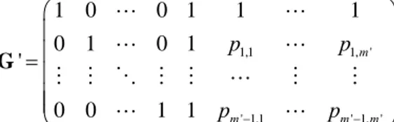
LH*RS files may differ by their group size m and availability level k. Smaller m speed up the recovery time, but increase the storage overhead, and vice versa. The parity matrix P for a bucket group needs m rows and k columns, k = K or k = K –1. Different files in a system may need in this way different matrices P. We show in Section 4.2 that the choice of GF(2f)limits the possibilities for any P to m + k ≤ 2f + 1. Except for this constraint, m and k can be chosen quite arbitrarily. We also prove that for any parity matrix P’ with dimensions m’ and k’, every m < m’ by k < k’ top left corner of P’ is also a parity matrix. These properties govern our use of the parity matrices for different files. Namely, we use a generic parity matrix P’ and its logarithmic parity matrix Q’ in an LH*RS file system. The m’ and k’ dimensions of P’ and Q' should be big enough for any system application. Any actual P and Q we use are then the m ≤ m’ by k ≤ k’ top left corners of P’ and of Q’. Their columns are derived dynamically when needed.
Section 4.2 below shows the construction of our P’ for GF(28), (within the generator matrix containing it). We have to respect the condition that m’ + k’ ≤ 257. Because of LH*RS specifically, m’ has to be a power of two. Our choice for m’ was therefore
m’ = 128, to maximize the bound on the group size while allowing k’ > 1. Hence, k’ = 129. Figure 16 displays the 20 leftmost columns of Q’. Figure 17 displays these
columns of P’. The selection suffices for 20-available files. We are not aware of any application that needs higer level of availability.
As we said, we finally applied GF(216). P’ may then reach m’ = 32K by k’ = 32K + 1. This allows LH*RS files with more than 128 buckets per group. Ultimately, even a very large file could consist of a single group, if such an approach would ever prove useful.
Example 2
We continue to use GF(28) and the conventions of Section 3.1. We now illustrate the encoding principles presented until now, by the determination of the parity data that
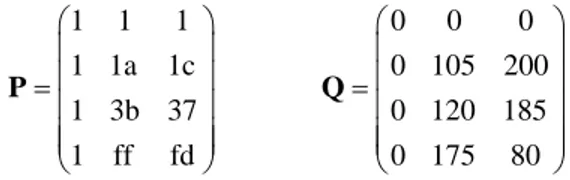
should be in k =3 parity records for the record group of size of m = 4 whose description follows. Figure 5 shows P and Q. These are the top left four rows and three columns of P’ and Q’ in Figure 17 and Figure 16.
1 1 1 0 0 0 1 1a 1c 0 105 200 1 3b 37 0 120 185 1 ff fd 0 175 80 ⎛ ⎞ ⎛ ⎞ ⎜ ⎟ ⎜ ⎟ ⎜ ⎟ ⎜ ⎟ = = ⎜ ⎟ ⎜ ⎟ ⎜ ⎟ ⎜ ⎟ ⎜ ⎟ ⎜ ⎟ ⎝ ⎠ ⎝ ⎠ P Q
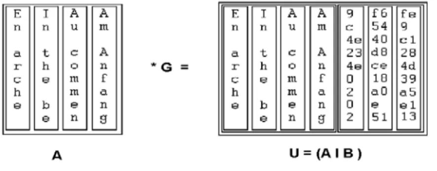
Figure 5: Matrices P and Q derived from P’ and Q’ for a 3-available record group of size m = 4. We suppose the encoded data records to have the non-key fields as follows: “En arche en o logos …”, “In the beginning was the word …”, “Au commencement était le mot …”, and “Am Anfang war das Wort…”. Using ASCII coding, these strings translate to (hex) strings of our GF symbols: “45 6e 20 61 72 63 68 …”, “49 6e 20 74 68 65 20 …”, “41 75 20 63 6f 6d 6d …”, and “41 6d 20 41 6e 66 61 …” To calculate the first parity symbols, we form the vector a0 = (45,49,41,41) and multiply it with P. The result b0 = a0⋅P is (c, d2, d0). We calculate the 1st symbol of b0 simply as 45 + 49 + 41 + 41 = c. This is the conventional parity, as in a RAID. The calculation of the parity second symbol is in fact given in Example 1. We use formally the second column of P and the
GF multiplication to obtain:
(
45 49 41 41) (
1 1a 3b ff)
45 1 49 1a 41 3b 41 ff 45 4 5d ce d2. T • = ⋅ + ⋅ + ⋅ + ⋅ = + + + =In our implementation, we use Q and the ‘*’ multiplication between two GF elements (or matrices) when the right operand is a logarithm. This yields, according to Table 1:
(
45 49 41 41) (
0 105 120 175)
45* 0 49 *105 41*120 41*175
45 antilog(log(49)+105) antilog(log(41)+120) antilog(log(41)+175)
= 45 + antilog(152 105) antilog(191 120) antilog(191+175)
= 45 + antilog(257) antilog(311 T ∗ = + + + = + + + + + + + + ) antilog(191+175) 45 04 5d ce d2 + = + + + =
Analogously, we get the last element in b0. The calculus iterates for b1 = (18,76,93), b2 = (0,e2,ff) …. As the result, the B-field in the 1st parity record, Figure 1, is encoded as B = “c 18 0…”. Likewise, the second B-field is “d2 76 e2…” and the third one is finally “d0 93 ff…”.
3.3 Parity Updating
The application updates an LH*RS file a data record at a time. An insert, update or delete of a record, modifies the parity records of a record group. We call this parity updating. It is the actual calculus for the parity encoding in the LH*RS files. We now introduce these principles.
We formally assimilate an insert and a deletion to specific cases of the update that is here our generic operation. Recall, we only operate in fact on the non-key fields. An insert changes the record from a zero string. A deletion does the opposite. We now consider an update in this way to the ith data record in its group. Let matrix A of vectors a in Section 4.2 above be the symbols in the data records in the record group before the update. Let matrix A’ contain the symbols after the update. The matrices only differ in the ith column. Let B and B’ be the matrices of vectors b with the resulting parity codes.
The codes should conform to the generic calculus rules in Section 4.2. We thus have B = AP, B’ = A’P. The difference B - B’ is ∆ = (A A’) P. We have A A’ = (0,...,0,∆i,0,...,0) where ∆i is the column with the differences between the same offset symbols in the former and new records. To calculate ∆ = (A - A’)P, we only need the ith row of P. Since B’ = B + ∆, we calculate the new parity values by calculating ∆ first and then XOR this to the current B value. In other words, with Pi being the ith row of P:
(3.3) B’ = A’⋅G = (A+(A’-A)) P = A P + (A - A’) P = P + ∆i Pi.
In particular, if bj is the old symbol, then we calculate the new symbol b’j in record j as (3.4) b’j = bj + ∆i pi,j,
where ∆i is the difference between the new and the old symbol in the updated record, and
pi,j is the coefficient of P located in the ith row and jth column.
The ∆-record is the string obtained as the XOR of the new and the old symbols with the same offset within the non-key field of the updated record. For an insert or a delete, the ∆-record is the non-key data. We implement the parity updating operation resulting from an update of a data record with key c and rank r as follows. The LH*RS data bucket computes the ∆-record and sends it, together with c and r, to all the parity buckets of the record group. Each bucket sets the B field value according to (3.3). It then either updates the existing parity record r or creates it. Likewise, the data record deletion updates the B field of the parity record r or removes all records r in each parity bucket. We discuss these operations more in depth in Section 5.6 and 5.7.
for the encoding. A parity bucket stores therefore basically only this column. Obviously, the first parity bucket does not have to store p1 if it is the column of ones as above.
Notice that our parity updating needs only one data record in the group, i.e., the updated one. This property is crucial to the efficiency of the encoding scheme. In particular, update speed is independent of m. Its theoretical basis is that our coding scheme is systematic. We elaborate more on it while discussing alternate codes in Section 7.5.1.
Example 3
We continue with the running example. We consider a file of four data buckets D0, D1, D2, and D3 forming the bucket group of size m = 4. We also consider three parity buckets P0, P1, P2 corresponding to the columns of matrices P and Q in Figure 5. We now insert one by one the records from Example 2. We assume they end up in successive buckets and form a record group. At the end, we also update the record in D1. Figure 6 shows vertically each non-key field of a data record in the group, and the evolution of the B-fields, also represented vertically. It thus illustrates also the matrices A, A’ and B, and B’ for each parity updating operation we perform.
Figure 6a shows the insert into D0 of the 1st record, with non-key data “En arche ...”, i.e., (hex) “45 6e 20 61 72 63 68 65 20 65 ...”. The ∆-record is identical to the record, being the difference between this string and the previous non-key data string, which is here the zero string. The first row of P consisting of ones, we calculate the content of each parity bucket by XORing the ∆-record to its previous content. As there were no parity records for our group yet, each B-field gets the ∆-record and we create all three records.
Figure 6b shows the evolution after the insert of “In principio …” into D1. The ∆-record is again identical to the data ∆-record. At P0, the existing parity ∆-record is XORed with the ∆-record. At P1, we multiply the ∆-record by ‘1a’ and we XOR the result with the existing string. The ‘1a’ is the P-coefficient located in Figure 5 in the second row (corresponding to D1) and the second column (corresponding to P1). We update the parity data in P2 similarly, except that we multiply by ‘1c’.
Figure 6c-d show the evolution after inserts of “Am Anfang war …” into D2 and “Dans le commencement …” into D3. Finally, Figure 6e shows the update of the record in D0 to “In the beginning was …”. Here, the ∆-record is the XOR of “49 6e 20 74 68 65 20 62 65 67 …” and of “45 6e 20 61 72 63 68 65 20 65”, yielding “c 0 0 15 1a 6 48 7 45 67 …”. We send this ∆-record to the parity buckets. It comes from D0, so we only XOR
the ∆-record to the strings already there. D0 D1 D2 D3 P0 P1 P2 D0 D1 D2 D3 P0 P1 P2 45 0 0 0 45 45 45 45 49 0 0 c 41 ea 6e 0 0 0 6e 6e 6e 6e 6e 0 0 0 4b 32 20 0 0 0 20 20 20 20 20 0 0 0 47 87 (a) 61 0 0 0 61 61 61 (b) 61 70 0 0 11 75 48 72 0 0 0 72 72 72 72 72 0 0 0 52 63 63 0 0 0 63 63 63 63 69 0 0 a 0 6b 68 0 0 0 68 68 68 68 6e 0 0 6 4d 34 D0 D1 D2 D3 P0 P1 P2 D0 D1 D2 D3 P0 P1 P2 45 49 41 0 4d 1c 9c 45 49 41 44 9 f6 fe 6e 6e 6d 0 6d c 93 6e 6e 6d 61 c 54 09 20 20 20 0 20 74 29 20 20 20 6e 4e 40 c1 (c) 61 70 41 0 50 28 3e (d) 61 70 41 73 23 d8 28 72 72 6e 0 6e 58 9b 72 72 6e 20 4e ce 4d 63 69 66 0 6c cf 36 63 69 66 6c 0 18 39 68 6e 61 0 67 23 ec 68 6e 61 65 2 a0 a5 D0 D1 D2 D3 P0 P1 P2 49 49 41 44 5 fa f2 6e 6e 6d 61 c 54 9 20 20 20 6e 4e 40 c1 (f) 74 70 41 73 36 cd 3d 68 72 6e 20 54 d4 57 65 69 66 6c 6 1e 3f 20 6e 61 65 4a e8 ed
Figure 6: Example of Parity Updating Calculus.
4 DATA DECODING
4.1 Using Generator Matrix
The decoding calculus uses the concept of a generator matrix. Let I be an m x m identity matrix and P a parity matrix. The generator matrix G for P is the concatenation I|P. We recall from Section 3.2.1 that we organize the data records in a matrix A. Let U denote the matrix A⋅G. U is the concatenation (A|B) of matrix A and matrix B from the previous section. We refer to each line u = (a1, a2,..., am, am+1, ..., an) of U as a code
word. The first m coordinates of u are the coordinates of the corresponding line vector a
in the record group. The remaining k coordinates of u are the newly generated parity codes. A column u’ of U corresponds to an entire data or parity record.
A crucial property of G is that any m by m square submatrix H is invertible. (See Section 4.2 for the proof.) We use this property for reconstructing up to k unavailable data or parity records. Consider first that we wish to recover only data records. We form a matrix H from any m columns of G that do not correspond to the unavailable records. Let S be A⋅H. The columns of S are the m available data and parity records we picked in order to form H. Using any matrix inversion algorithm, we compute H-1. Since A⋅H = S, we have A = S⋅H-1
. We thus can decode all the data records in the record group. Hence, we can decode in particular our k data records. In contrast, we cannot perform the decoding if more than k data or parity records are unavailable. We would not be able to form any square matrix H of size m.
Figure 7: Definition of matrices A, B, U.
In general, if there are unavailable parity records, we can decode the data records first and then re-encode the unavailable parity records. Alternatively, we may recover these records in a single pass. We form the recovery matrix R = H-1⋅G. Since S = A⋅H, we have A = S⋅H-1, hence U = A⋅G = S⋅H-1⋅G = S⋅R. Although the recovery matrix has m rows and n columns, we only need the columns of the unavailable data and parity records.
Our basic scheme in the prototype uses Gaussian elimination to compute H-1. It also decodes data buckets before recovering parity buckets. Our generic matrix P’ has 128 rows and 129 columns for GF (256). As we said, to encode a group of size m < 128, we cut a submatrix P of size m x m. To apply P’ in full is possible, but wastes storage and calculation time, since all but m first symbols in each line of A and B are zero. Hence the elements of P’ other than in top left m x m submatrix would not serve any purpose.
especially, the inversion of full size H derived from the generic generator matrix G’ = I|P’. This despite the fact that as for the encoding using P’, the elements of H-1 other than those in the top left m x m submatrix of H-1 would not contribute to the result. Storing and inverting a 128 x 128 matrix is more involved than a smaller one. It would be more efficient to create the m x m submatrix Hand invert only H. This requires however that the cut and the m by m inversion leads to the same submatrix H-1 as that derived by the full inversion followed by the m x m cut. Fortunately, this is the case.
Proof. Consider that for the current group size m < m’. There are m’ - m dummy data
records padding each record group to size m’. Let a be the vector of m’ symbols with the same offset in the data records of the group. The rightmost m’ - m coefficients of a are all zero. We can write a = (b|o), where b is an m-dimensional vector and o is the m’-m dimensional zero vector. We split G’ similarly by writing:
0 1
'
G
G
G
⎛
⎞
= ⎜ ⎟
⎝
⎠
.Here G0 is a matrix with m rows and G1 is a matrix with m’ - m rows. We have u = a⋅G = b⋅G0 + o·G1 = b⋅G0. Thus, we only use the first m coefficients of each row for encoding.
Assume now that some data records are unavailable in a record group, but m records among m + k data and parity records in the group remain available. We can now decode all the m data records of the group as follows. We assemble the symbols with offset l from the m available records, in a vector bl. The order of the coordinates of bl is the order of columns in G. Similarly; let xl denote the word consisting of m data symbols with same offset l from m data records, in the same order. Some of the values in xl are from the unavailable buckets and thus unknown. Our goal is to calculate x from b.
To achieve this, we form an m’ by m’ matrix H’ with at the left the m columns of G’ corresponding to the available data or parity records and then the m’-m unit vectors formed by the column from the I portion of G’ corresponding to the dummy data buckets. This gives H’ a specific form:
'
H
O
H
Y
I
⎛
⎞
= ⎜
⎟
⎝
⎠
.Here, H is an m by m matrix, Y an m’-m by m matrix, O the m by m’ - m zero matrix, and I is the m’− m by m’ − m identity matrix. Let (xl
vector consisting of the m coordinates of xl and bl respectively, and m’− m zero coefficients.
( | )
x o
H
O
( | )
b o
Y
I
⎛
⎞
=
⎜
⎟
⎝
⎠
. That is:=
xA
b
.According to a well-known theorem of Linear Algebra, for matrices of this form det(H’) = det(H)⋅det(I) = det(H). So H is invertible since H’ is. The last equation tells us that we only need to invert the m-by-m matrix H. This is precisely the desired submatrix H cut out from the generic one. This concludes our proof.
Example 4
Consider the situation where the first three data buckets in Example 3 are unavailable. We collect the columns of G corresponding to the remaining four buckets in matrix:
0 1 1 1 0 1 1a 1c 0 1 3b 37 1 1 ff fd ⎛ ⎞ ⎜ ⎟ ⎜ ⎟ = ⎜ ⎟ ⎜ ⎟ ⎜ ⎟ ⎝ ⎠ H . We invert H to obtain: 1 1 a7 a7 1 46 7a 3d 0 . 91 c8 59 0 d6 b2 64 0 − =
⎛
⎞
⎜
⎟
⎜
⎟
⎜
⎟
⎜
⎟
⎝
⎠
HThe fourth column of H-1 is a unit vector, since the fourth data record is among the survivors and we need not calculate it. To reconstruct the first symbol in each data bucket simultaneously, we form vector b from the first symbols in the surviving buckets (D3, P0, P1, P2): b = (44, 5, fa, f2). This vector is the first row of the matrix B. We multiply b⋅H-1
and obtain (49,49,41,44), which is the first row of matrix A. We iterate over the lines of B to obtain the other rows of A.
4.2 Constructing a Generic Generator Matrix
We now show the construction of our generic generator matrix G’, illustrated in Figure 9. Matrix G used in Example 4 above is derived from G’. The construction provides also
our matrix P’ as a byproduct. Let aj be l elements of any field. It is well known, see, e.g. [MS97], that the determinant of the l-by-l matrix that has the ithpower of element aj in row i and column j is:
(4.1)
( )
0 , 1 0 1det
ij(
j i)
i j l i j la
a
a
≤ ≤ − ≤ < ≤ −=
∏
−
.If the elements ai are all different, then the determinant is not zero and the matrix invertible.
We start constructing G’ by forming a matrix V with n + 1 columns and m’ rows, Figure 8. The first n columns contain the successive powers of all the different elements in the Galois field GF(n) starting with 0. The first column has a 1 in the first row and zeroes below. The final column consists of all zeroes but for a 1 in row m’ − 1. V is the
extended Vandermonde matrix [MS97, p.323]. It has the property that any submatrix S
formed of m’ different columns is invertible. This follows from (4.1), if S does not contain the last column of V. If S contains the last column of V, then we can apply (4.1) to the submatrix of S obtained by removing the last row and column of V. This submatrix has the determinant of S and is invertible, so S is invertible.
We transform V into G’, Figure 9, as follows. Let U be the m’ by m’ matrix formed by the leftmost m’ columns of V. We form an intermediate matrix W = U-1⋅V. The leftmost m’ columns of W form the identity matrix, i.e. W has already the form W = I|R. If we pick any m’ columns of W and form a submatrix S, then S is the product U-1⋅T with T the submatrix of V picked from the same columns as S. Hence, S is invertible. If we transform W by multiplying a single column or a single row by a non-zero element, we retain the property that any m’ by m’ submatrix of the transformed matrix is still invertible. The coefficients wm’,i of W located in the leftmost column of R are all non-zero. If this were not the case, and wm’,j = 0 for any index j, then the submatrix formed by the first m’ columns of W with the sole exception of column j and the leftmost column of R would have only zero coefficients in row j. It hence would be singular which would be a contradiction.
We now transform W into our generic generator matrix G’ first by multiplying all rows j with wm’,j-1. As a result of these multiplications, column m’ now only contains coefficients 1? But the left m’ columns no longer form the identity matrix. Hence we multiply all columns j ∈ {0,… m’-1} with wm’,j to recoup the identity matrix in these columns. Third, we multiply all columns m’,... n with the inverse of the coefficient in the first row. The resulting matrix has now also 1-entries in the first row. This is our generic
generator matrix G’.
We recall that the record group size for LH*RS is a power of 2. For the reasons already discussed for P’, for GF(256), our I’ matrix is 128 by 128 and P’ is 128 by 129. Hence, our G’ is 128 by 257. Notice the absence of need to store I’ or even I.We recall also that Figure 17 shows the leftmost 20 columns of P’ produced by the algorithm using the above calculus. Likewise, Figure 14 shows a fragment of P’ computed for GF(216). Finally, notice that there is no need to store even these columns. At the recovery, they can be obviously dynamically reconstructed from columns of Q’ or Q, available for the encoding anyway. 0 0 0 1 2 1 1 1 1 1 2 1 1 2 2 1 2 1 ' 1 ' 1 ' 1 1 2 1 1 0 0 0 0 0 0 1
V − − − − − − − =
⎛
⎞
⎜
⎟
⎜
⎟
⎜
⎟
⎜
⎟
⎜
⎟
⎜
⎟
⎝
⎠
L L L M M M O M M L n n n m m m n a a a a a a a a a a a aFigure 8: An extended Vandermonde matrix V with m’ rows and n=2f+1 columns.
1,1 1, ' ' 1,1 ' 1, ' 1 0 0 1 1 1 0 1 0 1 ' 0 0 1 1 m m m m p p p − p − ⎛ ⎞ ⎜ ⎟ ⎜ ⎟ =⎜ ⎟ ⎜ ⎟ ⎜ ⎟ ⎝ ⎠ G L L L L M M O M M L M M L L
Figure 9: Our generic generator matrix G’. Left m’ columns form the identity matrix I. The P’ matrix follows, with first column and row of ones.
5 LH*RS FILE MANIPULATION
The application manipulates an LH*RS file as an LH* file. The coordinator manages high-availability invisibly to the application. Internally, each bucket access starts in normal mode. It remains so as long as the bucket is available. Bucket availability means here that the SDDS manager at the node where the bucket resides responds to the message. If a node carrying a manipulation encounters an unavailable bucket a, it enters
degraded mode. The node passes the manipulation then to the coordinator. The
coordinator manages the degraded mode to possibly complete the manipulation. It initiates the bucket recovery operation of bucket a, unless it is already in progress. It performs also some other operations specific to each manipulation handled to it that we show below. Operationally, the coordinator performs in fact the requested recovery of bucket a as a part of the bucket group recovery operation. The latter recovers all