HAL Id: tel-02084130
https://pastel.archives-ouvertes.fr/tel-02084130
Submitted on 29 Mar 2019
HAL is a multi-disciplinary open access archive for the deposit and dissemination of sci-entific research documents, whether they are pub-lished or not. The documents may come from teaching and research institutions in France or abroad, or from public or private research centers.
L’archive ouverte pluridisciplinaire HAL, est destinée au dépôt et à la diffusion de documents scientifiques de niveau recherche, publiés ou non, émanant des établissements d’enseignement et de recherche français ou étrangers, des laboratoires publics ou privés.
Spontaneous decoherence in large Rydberg systems
Eric Magnan
To cite this version:
Eric Magnan. Spontaneous decoherence in large Rydberg systems. Optics [physics.optics]. Université Paris Saclay (COmUE), 2018. English. �NNT : 2018SACLO008�. �tel-02084130�
R É S U M É
De nombreux phénomènes de la vie quotidienne sont bien plus subtils qu’ils n’y paraissent. C’est le cas par exemple du magnétisme, qui, bien que très simple en apparence, se révèle très complexe à l’échelle atomique. En pratique, même les modèles les plus simples demandent rapidement une puissance de calcul bien supérieure à celle des supercalculateurs ac-tuels.
Pour contourner cet obstacle, une alternative consiste à remplacer le calcul par la mesure d’un système expérimental se comportant comme le modèle : c’est la simulation quantique. Cette technique a été propo-sée pour étudier un vaste panel de problèmes, allant du rayonnement de Hawking à la thermodynamique quantique, avec différentes plateformes expérimentales telles que les ions, photons ou gaz d’atomes froids.
La simulation quantique permet notamment d’étudier des phases exo-tiques de la matière, comme par exemple les rotons, solitons, supersolides ou encore les phases topologiques. Ces phases n’apparaissent pas sponta-nément dans les gaz d’atomes alcalins, mais plusieurs travaux théoriques ont montré qu’elles peuvent émerger en présence d’interactions à longue portée.
Pour augmenter la portée des interactions dans un échantillon atomique, une solution consiste à exciter les atomes dans des états électroniques n de haute énergie appelés états de Rydberg. Ces états ont une interaction de type van der Waals, laquelle évolue rapidement avec le niveau d’énergie (UvdW Ã n11). Cependant, ces états ont une durée de vie trop courte pour
permettre d’observer les nouvelles phases (voir Fig.1a).
Ce problème peut être résolu en mélangeant de manière cohérente une petite fraction Á π 1 d’états de Rydberg |rÍ avec une fraction plus large d’atomes dans l’état fondamental |gÍ. Le mélange qui en résulte |ÂÍ = (1≠ Á)|gÍ+Á|rÍ combine long temps de vie et large portée d’in-teractions (voir Fig.1b). Cette proposition d’habillage Rydberg offre ainsi
une solution expérimentale pour observer de nouvelles phases de la ma-tière dans des échantillons d’atomes alcalins.
Cette idée a suscité un vaste intérêt dans la communauté scientifique et a conduit à de nombreuses études théoriques. L’habillage Rydberg a été appliqué avec succès sur un système de deux atomes (voir Fig.1c), mais
la même technique appliquée à des systèmes plus larges n’a pas produit les résultats escomptés.
A C K N O W L E D G M E N T S
I acknowledge the support of the National Science Fundation via the Physics Frontier Center at Joint Quantum Institute. This PhD was also supported by the Fulbright Program via the Commission Franco-Américaine and the Institut d’Optique.
I warmly thank my jury : Isabelle Bouchoule, Olivier Gorceix, Shannon Whitlock and Daniel Comparat.
I am obliged to my two advisors, Trey Porto and Antoine Browaeys, for giving me the opportunity to work in their teams. I also thank Luis Orozco who made this PhD possible, and Thierry Lahaye who kindly men-tored me during this past year.
I which to express my gratitude to the other teams, namely Rb1, RbRy, Chadoq and Cyclopix. It’s been a pleasure working with you, guys.
I warmly thank Timothée Cognard, Hélène Arvis, Lara Ehrenhofer and Nudrat Piracha, who have been my partners in crime in many adventures. Thanks for your encouragements!
And finally, a very special gratitude to my family: I owe it all to you.
A N O T E T O T H E J U RY
In 2015, I had the opportunity to do a joint Ph.D. between Trey Porto’s and Antoine Browaeys’ laboratories. Both experiments focus on quantum simulation using atoms in the Rydberg state: while the American ex-periment studies dissipation in large ensembles, the French exex-periment investigates the dynamics of smaller ensembles.
I started my Ph.D. in January 2016 at the Joint Quantum Institute (JQI) and stayed there for two years. We identified an avalanche decoher-ence mechanism affecting large Rydberg ensembles: this work had a large resonance in the cold atom community as it calls into question dozens of proposals. In January 2018, I joined the team at Laboratoire Charles Fabry at Institut d’Optique (LCFIO) to work on an evolution of their “atom-by-atom assembler”. This new setup aims to eliminate the black-body radiation at the origin of the broadening mechanism. Our goal is to make sure that large structures assembled on the tweezer-based exper-iment will not be affected by the decoherence.
As cold atoms experiments always correspond to a collective effort, it may be difficult to identify my contributions. Below is a list of some of my achievements as a graduate student.
— In early 2015, the experiment had just been move from the N.I.S.T building and was still to be reassembled. After Bose-Einstein con-densation was achieved, I was in charge of the Rydberg excitation. In particular, we took the opportunity to modernize the setup. — Later that year, I dedicated some significant amount of time to the
double-wells optical lattice. We did not get to use this tool to its full capacity that year, but we achieved to get balanced sublattices. — While the first publication concerning the decoherence in Rydberg
ensembles was published before my arrival[60], I built the optics and
took the data for the two next publications[24, 149].
— I built and characterized the “piezo-mirrors” currently used on the JQI experiment for Floquet excitation (see App.A).
— At LCFIO, I assembled from scratch a new experimental setup for cold atom experiments under the supervision of T. Lahaye. I also performed series of tests in an optomechanical mount at 77 K.
Palaiseau, France, October 2018
P U B L I C AT I O N S
Publications by the author
T. Boulier et al., “Parametric instabilities in a 2D periodically-driven bosonic system: Beyond the weakly-interacting regime”, submitted to
PRX (2018) (arXiv:1808.07637)
E. Magnan et al., “A low-steering piezo-driven mirror.”, RSI 89, 073 110 (2018). (doi: 10.1063/1.5035326)
J.T. Young et al., “Dissipation induced dipole blockade and anti-blockade in driven Rydberg systems”, PRA 97,023 424 (2018). (doi: 10.1103/Phys-RevA.97.023424)
T. Boulier et al. “Spontaneous avalanche dephasing in large Rydberg en-sembles”, PRA 96 053 409 (2017). (doi: 10.1103/PhysRevA.96.053409)
Other relevant publications for this work
E. A. Goldschmidt et al., “Anomalous Broadening in Driven Dissipa-tive Rydberg Systems.”, PRL 116, 113 001 (2016) (doi: 10.1103/Phys-RevLett.116.113001)
J. E. Johnson and S. L. Rolston “Interactions between Rydberg-dressed atoms.”, PRA 82, 033 412 (2010) (doi: 10.1103/PhysRevA.82.033412)
I N T R O D U C T I O N
Many phenomena observed in condensed matter physics are still not properly understood today. Physicists are able to write simplified theoret-ical models that capture the essence of the phenomena, but these models are still too complicated to be solved when the number of interacting particles is larger than a few tens[103]. This is especially true when the
interactions are long-range or when dissipation is present because the sys-tem is not well-enough shielded from the fluctuations of its environment.
The field of quantum simulation has emerged as one approach to solve these problems[55, 88]. It consists in building artificial experimental
sys-tems that are ruled by the idealized models proposed by the theorists. Measuring the properties of these engineered systems gives access to prop-erties of the model that is otherwise impossible to calculate.
Over the last 20 years, several experimental platforms for quantum simulation have been proposed, including superconducting circuits[121],
interacting photons[70], trapped ions[152] and cold atoms[19,76]. Among
them, laser-cooled atoms prepared in highly-excited “Rydberg” states are promising candidates[127, 145]. The van der Waals interaction between
two atoms scales as à n11 (where n is the principal quantum number),
allowing strong interactions even at interatomic distances of a few mi-crometers[53]. Moreover, the interaction is fully controllable with lasers
or static electric fields. Remarkably, the interaction can also be mapped onto spin Hamiltonians, which are relevant to many models proposed in condensed matter physics[83,147].
Among Rydberg-based quantum simulators, two different approaches have emerged. On one hand, atoms trapped in optical lattices allow to en-gineer large arrays of atoms with a fixed geometry where several thousands of particles are separated by intersite distances of 0.5 µm[84, 99]. On the
other hand, arrays of individual microtraps allow to produce mesoscopic structures of arbitrary geometry containing several tens of atoms at tun-able interatomic distances Ø 3 µm[10, 117]. These two solutions allow to
address the atoms individually, i.e. detect and manipulate each atom in-dependently of its neighbor.
Interatomic distances plays a major role in both types of simulators. In the case of atoms in individual microtraps, the large distances between the atoms requires to work at high Rydberg states (n > 50) in order
to get strong enough interactions. As the radiative lifetime scales with the Rydberg level (Ã n3), it can reach several hundreds of microseconds.
This timescale is much larger than the usual times of the experiment
xvi
(≥ 100 ns ≠ 1 µs) and allows to observe the coherent evolution of the en-semble of interacting atoms. This is an ideal system to explore interaction induced dynamics in an elementary closed many-body system.
On the opposite, atoms in optical lattices are much closer to each other and do not necessitate high levels of Rydberg states. Principal quantum numbers around n = 20 are typically sufficient to produce visible inter-actions. The typical lifetimes of such states is relatively short (5 µs) and can lead to dissipation and relaxation of the system. Relaxation to equilib-rium is predicted to hide interesting phenomena, notably the spontaneous formation of an antiferromagnetic order[98]. The model predicts an
oscil-lation between two anti-ferromagnetic configurations — seing this effect in the laboratory would be an experimental realization of an elementary open many-body system.
Both types of simulators are limited by the radiative lifetime of Rydberg states, leading to a regime where the atoms are effectively frozen in space during the experiment. However, major effects related to the mechanical motion of the atoms have been predicted to exist, notably non-linear dy-namics[110] and exotic phases such as supersolidity[107]. The timescale
of these effects is directly linked to the trapping frequencies of the optical lattice (typically in the kHz range), and thus requires atomic lifetimes in the range 1 ≠ 10 ms.
In recent years, “Rydberg-dressing” has been proposed as a solution to increase the lifetime of Rydberg ensembles by several orders of magnitude while maintaining relatively strong interactions[23,58,87]. The proposal
consists in coherently admixing a large fraction of ground state atoms with a small fraction of Rydberg states, resulting in a mixture combining long lifetime and long interaction ranges. While this approach has been successful with two atoms[86], deviations to the theory have been seen in
all experiments using larger ensembles[1, 46,54, 60].
In this thesis, we investigate the two types of Rydberg-based quantum simulators. In a first serie of experiments performed at Joint Quantum Institute (University of Maryland, USA), we study the physics of a Bose-Einstein Condensate loaded into optical lattices and excited to the 18S level. We show that the spontaneous apparition of a population in nearby Rydberg states triggers an avalanche of decoherence responsible for the anomalies observed in Rydberg dressing experiments in large ensembles. The decoherence emerges from stimulated emission induced by blackbody radiation followed by diffusion via resonant dipole-dipole interaction be-tween states of opposite parity. This type of physics being extremely complex, we use simple scalings based on mean-field approximations to analyze the effects.
xvii
We then investigate the time evolution of the several Rydberg popula-tions in the system. While some populapopula-tions can be directly measured by fluorescence, others require indirect schemes: we use a “pump-probe” technique to decouple the production of pollutant states from their obser-vation. Our measurements show a good agreement with mean-field models. Though Rydberg dressing does not seem applicable for large scale quan-tum simulators, we show that the decoherence can be mitigated to some extent by several simple techniques such as stroboscopic excitation or us-ing cut-off cavities. The use of a cryostat to inhibit blackbody radiation emerges as a particularly efficient solution, at the cost of being technically demanding.
Experiments performed in an array of microtraps at the Laboratoire Charles Fabry at Institut d’Optique (Palaiseau, France) show that the size of the atomic structures is limited by two-body collisions with the background residual gas. Using a cryostat could reduce the pressure by several order of magnitude in a process called cryopumping, where gaseous particles freeze at the contact of cold walls and stick to them. However, this types of experiment uses optomechanical components under vacuum: their adaptation to a cryogenic environment is bound to be challenging. We present the first investigations concerning the optomechanical design at 4 K.
This thesis is divided as follows:
a. The first part (see Part.i) is an introduction to the techniques of atom cooling and trapping and Rydberg excitation. While Ch.1
provides some details about the production of ultracold gases in optical lattices, Ch.2is dedicated to the physics of Rydberg states.
b. The second part (see Part.ii) covers experimental investigations of the spontaneous onset of decoherence in large Rydberg ensembles done at JQI at University of Maryland. In Ch.3, we detail
steady-state observations, Ch.4 explores the time evolution of the Rydberg
populations.
c. The third part (see Part.iii) concerns the design of a new apparatus using a 4 K cryostat with high-precision optomechanical components inside. This work was done at LCFIO. Our first tests are gathered in Ch.5.
C O N T E N T S
i a homogeneous gas of ultracold atoms with
tunable interactions 3
1 ultracold atoms in deep optical lattices 5
1.1 Optical traps for neutral atoms . . . 6
1.1.1 Energy lightshifts . . . 6
1.1.2 Harmonic traps . . . 7
1.1.3 Optical lattices . . . 9
1.2 Bose-Einstein Condensation . . . 11
1.2.1 Condensation in a cubic box . . . 12
1.2.2 Condensation in a harmonic potential . . . 13
1.3 Loading Bose-Einstein Condensates in deep lattices . . . . 13
1.3.1 Bose-Hubbard model . . . 14
1.4 Experimental setup . . . 15
1.4.1 Magnetic equipment . . . 15
1.4.2 Initial cooling equipment . . . 15
1.4.3 Magnetic timeout . . . 16
1.4.4 Evaporative cooling system . . . 17
1.4.5 Imaging system . . . 17
1.5 An exotic optical lattice . . . 19
1.5.1 Intrinsic phase-stability . . . 20
1.5.2 Loading ultracold atoms into the optical lattice . . 21
1.5.3 Controlling the atomic density . . . 22
2 rydberg atoms 23 2.1 Generalities . . . 24
2.1.1 Quantum defect theory . . . 24
2.1.2 Rydberg lifetimes . . . 25
2.2 Interactions between Rydberg atoms . . . 27
2.2.1 van der Waals and dipole-dipole regimes . . . 27
2.2.2 Rydberg blockade . . . 28
2.2.3 Chosing the Rydberg state for our experiment . . . 30
2.2.4 Interactions between 18S and nP atoms . . . . 31
2.3 Experimental production of Rydberg atoms . . . 33
2.3.1 Two-level excitation scheme . . . 33
2.3.2 Ultrastable cavity . . . 33
2.3.3 Rydberg lasers . . . 34
2.3.4 Calibrations of the Rabi frequency . . . 35
2.3.5 Detection of Rydberg atoms . . . 37
2.3.6 Towards experimentations . . . 39
xx contents
ii spontaneous dephasing in large rydberg
en-sembles 41
3 anomalous broadening in large rydberg
ensem-bles 43
3.1 Elements of theory: Rydberg dressing . . . 44
3.1.1 A naive approach to Rydberg dressing . . . 44
3.1.2 Rydberg dressing in a pair of atoms . . . 45
3.1.3 Experimental implications . . . 47
3.2 Rydberg dressing in large ensembles . . . 49
3.2.1 Experimental parameters . . . 49
3.2.2 Experimental observables . . . 49
3.2.3 Initial observations . . . 51
3.3 Shortlisting the broadening causes . . . 54
3.3.1 Microscopic arrangement . . . 54
3.3.2 Lifetime measurement . . . 55
3.4 Steady-state scalings . . . 57
3.4.1 Van der Waals scaling . . . 57
3.4.2 Dipole-dipole scaling . . . 59
4 investigations of the dynamics of the rydberg populations 63 4.1 Dynamics of the nS population . . . . 65
4.1.1 Mean-field modeling . . . 65
4.1.2 Dynamics of the nS population . . . . 67
4.1.3 A stroboscopic experiment . . . 69
4.2 Dynamics of the nÕP population . . . 71
4.2.1 A pump-probe technique . . . 71
4.2.2 Steady-state cross-broadening . . . 72
4.3 Dynamical cross-broadening . . . 76
4.3.1 Cross-broadening homogeneous mean-field model . 76 4.3.2 Dynamical cross-broadening experiment . . . 77
4.4 Possible workarounds . . . 79
4.4.1 Stroboscopic approach . . . 80
4.4.2 Microwave cavities . . . 80
4.4.3 Cryognenic temperatures . . . 82
4.5 Perspectives for Rydberg dressing . . . 86
iii rydberg atoms in a cryostat 87 5 designing cryogenic rydberg experiment 89 5.1 Arbitrary structures up to 72 atoms . . . 90
5.1.1 Pairs of interacting Rydberg atoms . . . 90
5.1.2 Building arbitrary arrays of microtraps . . . 91
5.1.3 An atom-by-atom assembler . . . 93
5.1.4 Building synthetic 3D structures . . . 95
5.2 Towards structures of Ø 300 atoms . . . 95
5.2.1 Motivations . . . 95
5.2.2 Limitations of the current setup . . . 96
contents xxi
5.3 First steps of a cryogenic assembler . . . 101
5.3.1 A new cold atoms apparatus . . . 101
5.3.2 Choice of a cryocooler . . . 104
5.4 Aspheric lenses in a cryostat . . . 106
5.4.1 Challenges . . . 106
5.4.2 A cost-effective testing system . . . 107
5.4.3 Thermal deformation of the mount . . . 108
5.4.4 Stress in the lenses . . . 110
5.4.5 Further development of the cryogenic experiment . 111
iv appendix 115
a appendix a: publication 117
b appendix b: technical drawings for a first
op-tomechanical mount 125
Part I
A H O M O G E N E O U S G A S O F U LT R A C O L D
AT O M S W I T H T U N A B L E I N T E R A C T I O N S
1
U LT R A C O L D AT O M S I N D E E P O P T I C A L L AT T I C E S
The experimental platform of this thesis work consists in a ho-mogenous frozen ideal gas of ultracold atoms.
Using a magneto-optical trap followed by evaporative cooling, we bring a thermal vapor down to quantum degeneracy (see Sec.1.2). The resulting in Bose-Einstein condensate (BEC) has a macroscopic size and exhibits purely quantum properties. Because of its accessibility and tunability, this state of matter is an excellent platform to probe quantum physics[40].
Optical lattices are periodic patterns of light resulting from the interference of two or more optical beams[18]. Trapping a
BEC into such a structure completely modifies its physics. In particular, increasing the depth of the lattice sites allows to ob-serve a quantum phase transition from a superfluid to a Mott-insulator[65, 84]. In our experiment, we load the BEC into a
very deep lattice, resulting in a cubic insulator close to unit filling (see Sec.1.3). The resulting sample, which has little to no interactions due to large interatomic distances (≥ 0.5 µm), is a homogeneous ideal gas of ultracold atoms. Long-range and well-controlled interactions can be added later on to the system in a process discussed Ch.2.
Over the years, the association of a BEC with optical lattices has led to a variety of experiments[17], notably including
exci-tation into the Rydberg state[104] or periodic shaking of the
optical lattice[151]. In particular, Bose gases in optical lattices
have become one of the most popular platforms for quantum simulation[19] and many-body quantum experiments[20].
In this chapter, we present the generic concepts involved in the preparation of the ideal gas. We use the dressed-state picture to introduce energy lightshifts and show that they can be used to generate taylor-made trapping potentials, such as harmonic traps and optical lattices (see Sec.1.1). We briefly explain the concept of Bose-Einstein condensation (see Sec.1.2) and show how ultracold atoms in deep lattices can form an interaction-free homogenous frozen gas (See sec.1.3). We finally provide a brief overview of our experimental apparatus (see Sec.1.4).
6 ultracold atoms in deep optical lattices
1.1
optical traps for neutral atoms
Among the many types of atom-photon interactions, we focus here on a conservative process called energy lightshifting. Using simple arguments, we recall how light affects the energy levels of a quantum system and show how this effect can be used to spatially confine atoms.
1.1.1
energy lightshifts
Let’s consider an atom as a two-level quantum system with ground state |gÍ, excited state |eÍ separated by an energy ¯hω0.
When immersing this atom into a light field, a possible approach con-sists in studying the system [atoms + photons in the mode][41].
Assuming N photons with energy ¯hω, the ground state |g, NÍ has an energy N ¯hω. After absorption of a photon, the excited state |e, N ≠ 1Í has an energy ¯hω0+ (N ≠ 1)¯hω. The interaction between the field and
the atom can be written ˆ V = ¯h Ω1(r) 2 1 ˆ σ+aˆ+σˆ≠aˆ† 2 (1) where ˆa an ˆa† are the usual creation and anihilation operators. The
exci-tation and decay operators ˆσ+ and ˆσ≠ define as
ˆ
σ+ =|eÍÈg| (2a)
ˆ
σ≠ =|gÍÈe| (2b)
Ω1(r) can be understood as the Rabi frequency at r when only one photon is in the mode.
The interaction ˆV can only couple states of the dressed atom of same multiplicity,
Èe, N ≠ 1| ˆV |g, NÍ= ¯hΩ1(r)
2 Ô
N (3)
We usually define it as the Rabi frequency as Ω, where
Ω(r) = Ω1(r)ÔN (4)
In the mutiplicity {|g, NÍ, |e, N ≠ 1Í}, the Hamiltonian writes ˆ H = ¯h 2 Q a ∆ Ω(r) Ω(r) ≠∆ R b+εN (5)
with εN = (N ≠ 1/2)¯hω+¯hω0/2 and ∆ = ω≠ ω0. We introduce the
mixing angle ϑ(r) as cos(2ϑ(r)) = Ò ∆ ∆2+Ω2(r) sin(2ϑ(r)) = Ω(r) Ò ∆2+Ω2(r) (6)
1.1 optical traps for neutral atoms 7
The eigenvectors of the previous hamiltonian define as
|1(N)Í =cos(Ë)|g, NÍ+sin(Ë)|e, N ≠ 1Í (7a) |2(N)Í =sin(Ë)|g, NÍ+cos(Ë)|e, N ≠ 1Í (7b) The energies associated to these eigenstates write
EN(r) =±ÁN ±
¯h 2
Ò
∆2+Ω2(r) (8)
where +is for the higher level and ≠ is for the lower level.
As we can see from Eq.(8), the energy levels are shifted by the
inter-action. This light-induced modification of the eigenenergies is usually referred as lightshifting. In the limit of large detunings |∆| ∫ |Ω(r)|, the
lightshift writes
V(r) =û¯hΩ 2(r)
4∆ (9)
where ≠ is for the higher level and +is for the lower level. As far as the ground state is concerned, the lightshift lowers the energy for red-detuned light ∆ < 0 and increases it for blue-detuned light ∆ > 0.
Figure 1 – Energy lightshift
Shifting of the energy levels of a two-level quantum system in the red-detuned case (∆<0).
1.1.2
harmonic traps
Atoms tend to localize at the minimum of their ground state energy. Combining this behavior with energy lightshifts, it is possible to induce forces and create trapping potentials with light. One of the simplest man-ner to engineer such trap consists in using a tightly focused gaussian beam.
8 ultracold atoms in deep optical lattices
In the semi-classical approach, the Rabi frequency can be directly re-lated to the electric field
¯hΩ(r) = ≠d0E(r) (10)
where d0 is the atomic dipole moment and E(r) the amplitude of the
elec-tric field at position r.
The irradiance of a tightly focused laser beam propagating along z writes I(r, z) = I0 A w0 w(z) B2 exp A ≠ 2r 2 w(z)2 B (11) where r2 =x2+y2, w
0is the waist of the beam and w(z)its 1/e2diameter
at position z, which writes
w(z) =w0
Ò
1+ (z/zR)2 (12)
where zR is the Rayleigh length and writes
zR =
πω20
λ (13)
Introducing the impedance of free space η, the Rabi frequency corre-sponding to a gaussian beam can be written
Ω2(r) = d
2 0I(r)
2η ¯h2 (14)
Combining Eq.(9), (11) and (14) and assuming r2 π w02, the energy shift
of the atomic ground state induced by a gaussian beam writes
Vharm(r, z) =V0 A w0 w(z) B2A 1 ≠ 2w(rz2)2 B (15) where V0 =d20I0/(8∆η ¯h).
In the case of a red-detuned laser (∆ < 0), the potential is minimum at r=0, so that the atoms localize at the maximum of intensity (see Fig.2).
The trap depth is given by Vharm(r = 0, z = 0). In the case of cold
atoms, kT π V0, so that the atoms gather at the center of the trap. The
dipole potential can be approximated as a harmonic oscillator
Vharm(r, z) =≠V0 C 1 ≠ 23 r ω0 42 ≠ 3 z zR 42D (16) This type of trap is usually anisotropic and characterized by its trapping frequencies, which define as ωr = (4V0/mω02)1/2 and ωz = (2V0/mzR2)1/2
1.2 bose-einstein condensation 11
Figure 4 – Examples of optomechanical setups for optical lattices Two independent crossed beams lead to an array of tubes (a), adding a third pair of beams produces a tridimensional array (b). The vertical spacing can be magnified by crossing the vertical beams at a non-zero angle (c). The lasers beams are in red, the mirrors in dark grey, the lenses in light gray.
1.2
bose-einstein condensation
Optical and magnetic trapping allow to cool neutral atoms to extremely low temperatures. Starting in the middle of the 1980s, remarkable ad-vances in these techniques led to the discovery of a new phase of matter: Bose-Einstein condensates.
In this section, we show that bosons exhibit a gregarious behavior at low temperature and that a significant fraction of a bosonic ensemble can reach quantum degeneracy. This process, called Bose-Einstein Condensa-tion, was initially predicted by S. Bose and A. Einstein in 1924[22, 49].
A major argument of the theory is the indistinguishability of bosons, a property that implies strong deviations from Boltzmann statistics. Pro-ducing a Bose-Einstein Condensate requires extremely low temperatures, a condition that can be met with optical traps.
The canonical derivation of Bose-Einstein condensation involves sta-tistical mechanics and thermodynamics[40]. The starting point of the
demonstration consists in evaluating the average occupancy of a state j with energy Ej for a bosonic sample of N particles at temperature T
and chemical potential µ. This number is given by the Bose-Einstein law, which writes[66]
Nj = 1
12 ultracold atoms in deep optical lattices
1.2.1
condensation in a cubic box
Assuming a homogenous ideal gas of N identical bosons of mass m in a cubic box of typical size L, the eigen-states are plane waves characterized by their impulsion p= ¯hk and eigen-energies
Ep = |p| 2 2m (22) with p= 2fi ¯h L n (23)
with n = (nx, ny, nz) œ Z3. The ground state corresponds to p =0 and
E0 =0.
Using Eq.(21), it is possible to evaluate the average number of particles
in the state p and
Np =
1
e(Ep≠µ)kBT ≠ 1 (24)
and the total number of particles
N =ÿ
p
Np (25)
For each Np to be positive, Eq.(24) imposes µ < E0. Since the
condensa-tion corresponds to a gathering in the state of lowest energy, we decompose the total number of particles between the ones in the ground state (N0)
and the ones in all excited states (Nexc). We find
N0 = Z
1 ≠ Z (26)
with the fugacity Z =exp(µ/kBT). Since µ is negative, 0 < Z < 1. This
implies an upper boundary for Nexc.
Nexc< Nexc(max)(T) =
ÿ
p”=1
1
exp(Ep/kBT)≠ 1
(27) In three dimensions, this sum is finite. Bose-Einstein condensation is predicted by this very upper boundary: one expect a gathering of N0(T) =
N ≠ Nexc(max)(T) particules in the ground state. This result is a major
deviation from Boltzmann statistics, which only predicts an accumulation of particles in the ground state in the absence of thermal activation.
1.3 loading bose-einstein condensates in deep lattices 13
1.2.2
condensation in a harmonic potential
The previous reasoning can be applied to many types of potentials such as harmonic potentials.
Assuming a harmonic trap with typical trapping frequency ¯ω = (ωxωyωz)1/3,
the corresponding energy levels are non-degenerate. We enumerate them using the index j œ N, which leads to their energies
Ej = 3 j+ 1 2 4 ¯h ¯ω (28)
The condition µ < E0 now becomes µ < 3¯h ¯ω/2. The upper bound for
the number of excited states becomes
Nexc(max)(T) = ÿ
nx,ny,nz”=0
1
exp[¯h(ωxnx+ωyny+ωznz))/kBT]≠ 1
(29) When increasing the number of particles (N æ Œ), the level spacing becomes smaller and smaller, so that the previous sum can be replaced by an integral, Nexc(max)(T) = ⁄⁄ ⁄ Œ 0 dnxdnydnz exp[¯h(ωxnx+ωyny+ωznz)/kBT]≠ 1 (30)
The previous integral reduces to
Nexc(max)(T) = ζ(3) A kBT ¯h ¯ω B3 (31) With this, we can extract the critical temperature of condensation, Tc,
kBTc =0.94 ¯h ¯ωN1/3 (32)
Tc typically variates from a few µK to a few hundreds of nK depending
on N and ¯ω.
1.3
loading bose-einstein condensates
in deep lattices
Bose-Einstein condensates are usually produced in harmonic traps. Due to the harmonic confinement, the density profile is gaussian. Atoms also interact with each other, mostly via two-body collisions. In this part, we show that confining ultracold atoms in an optical lattice can lead to the production of a homogeneous ideal gas of ultracold atoms.
For the purpose of this thesis, we require an ensemble of ultracold atoms free of any interactions and uniformly distributed in space. One way to do it consists in loading a Bose-Einstein Condensate into a deep optical lattice using the superfluid to Mott-insulator transition. In this process, we load one atom per site, each lattice site being separated by ≥ λ/2. Such distances are typically much larger than interatomic interactions ranges between atoms in the ground state, the gas is therefore free of interactions.
14 ultracold atoms in deep optical lattices
1.3.1
bose-hubbard model
Ultracold atoms in optical lattices can be described by the Bose-Hubbard Hamiltonian, which writes
ˆ H =≠J ÿ Èi,jÍ ˆ a†iaˆj+ ÿ i (Ái≠ µ)nˆi+ 1 2U ÿ i ˆ ni(nˆi≠ 1) (33)
where J is the hopping term capturing the tunneling of bosons between the traps and U is the onsite energy. This term is related to the scatter-ing length from contact interactions. µ is the chemical potential, Ái =
Vharm(ri) a correcting factor that takes in account the inhomogeneities
in the external trapping potential. In our case, this term captures the curvature of the harmonic trap.
In the limit J ∫ U, the atoms are delocalized over the entire lattice and the sample is superfluid. On the contrary, when U ∫ J, the atoms become strongly confined and the tunneling is negligible. It is possible to show that under these conditions, the configuration that minimizes the energy corresponds to unit filling: each site is occupied by only one atom for an appropriate density. This state is called the Mott-insulator phase. Both regimes minimize the energy of the system: it is possible to con-nect them adiabatically by slowly increasing the ratio U /J, i.e. progres-sively increasing the optical lattice depth. Experimentally, the depth is controlled by the optical power of the lattice light: higher optical power results in deeper optical lattice depths. A Mott insulator can thus be produced by performing an adiabatic passage from the superfluid to the Mott insulator phase by progressively ramping up the optical power of the lattice light.
Superfluid and Mott-insulator phases are not specific to quantum gases: superfluidity has been encountered in4He[89] and the Mott insulator has
been originally developed to explain anomalous insulation in metal oxy-des[116].
1.4 experimental setup 15
1.4
experimental setup
This section is dedicated to the experimental setup developed at JQI. The apparatus involves generic methods to cool atoms down to quantum degeneracy. The experiment was first built in the 2000s[102] but went
through deep modifications ten years after[32]. Notably, the entire
appa-ratus was moved from the NIST (Gaithersburg, MD) to the JQI at Univer-sity of Maryland (College Park, MD) in October 2015. The reconstruction started shortly before my arrival at JQI. During my first months in the team, I participated to the assembly of the scientific features (notably the Rydberg setup, described in Chapter 2and the optical superlattice).
As far as BEC production is concerned, the apparatus is a relatively standard machine. Yet, two major peculiarities deserve to be pointed out:
1. The experiment uses a magnetic trap as a reservoir for a dipole trap. This system enables to overcome the usual magnetic trap limitations (notably Majorana spin-flip losses[28]) as well as those of the
far-detuned dipole trap (need for prohibitively high laser power). 2. Contrary to most BEC sequences, the BEC is held in a purely
mag-netic trap for a relatively long time (≥ 1 s) before the evaporative cooling. This “dark” stage allows to move bulky optical components and switch laser beams during this time.
1.4.1
magnetic equipment
The main chamber is a standard spherical octagon equipped with two independent sets of coils (see Fig.5). The top and bottom windows are
recessed.
A pair of anti-Helmoltz coils oriented along the vertical axis (z) and placed under vacuum generates a magnetic quadrupole. Under typical conditions, ˆzB = 0.12 T m≠1 for the MOT, and ˆzB = 0.48 T m≠1 for
the magnetic trap. Three additional pairs of coils are oriented along the main axes (x, y, z). Each pair is in the Helmholtz configuration and can produce a small magnetic shift.
1.4.2
initial cooling equipment
After being slowed down by a Zeeman slower, atoms enter the chamber from the left port and are captured by a magneto-optical trap (MOT) constituted of six independent laser beams in (see Fig.6) ≥ 5 cm diameter.
Under typical conditions, the slower laser and the Zeeman repumping lasers are respectively set to 30 mW and 15 mW. Once optimized, the MOT captures N = 9 ◊ 108 atoms in 3 s. The temperature of the cloud
1.5 an exotic optical lattice 19
ferred for quantitative analysis such as Kapitza-Dirac measurements[62] used to calibrate the lattice depth.
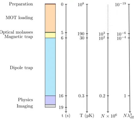
Overall, a typical BEC sequence takes approximately 16 s (see Fig.10),
most of the time being dedicated to the dipole evaporation. The total du-ration of the sequence can be slightly modified (notably the MOT loading time) depending on the quality of the vacuum pressure and the size of the BEC.
Figure 10 – Typical sequence to produce a BEC
1.5
an exotic optical lattice
The experiment at Joint Quantum Institute is equipped with an ex-otic optical lattice capable of generating pairs of double-wells[131]. Along
with the other types of tunable, non-cubic lattices (i.e. the Zurich exper-iment[138]), these optical lattices are often referred as superlattices.
Contrary to usual cubic lattices, the horizontal interference pattern is produced by a single laser folded onto a retro-reflected bowtie. Controlling the polarization allows to dynamically modify the interference pattern: if the beams are polarized along the lattice plane, they can only interfere with their retro-reflexion. This leads to a standard ⁄/2 lattice. However, when the polarization is orthogonal to the 2d-plane, all beams interfere, leading to a ⁄ lattice. The vertical interference pattern is produced by a pair of beams crossing at 20 degrees, which leads to a layer spacing of 2.34 µm.
20 ultracold atoms in deep optical lattices
Experimentally, the system includes two Pockels-cells which can vary the polarization of the light during the experiment (see Fig.11). We use
P ¥ 200 mW of ⁄= 813 nm laser light, which leads to intersite spacings of 813 and 407 nm for the two sublattices.
Figure 11 – Bowtie-shaped lattice
The relative intensity and positions of the two sublattices are con-trolled by two Pockels cells (Cylindrical black and white compo-nents) inserted between pairs of half-wave plates (in green).
1.5.1
intrinsic phase-stability
When engineering a superlattice, spatial drifts between the sublattices are a major concern. Small dephasing between the light beams, e.g. due to vibrational noise in the mirrors can lead to an uncontrolled deformation of the lattice pattern.
The bowtie structure is naturally phase-stable[131]: since any dephasing
affects all beams simultaneously, changing the phase translates the entire lattice without altering its structure.
The superlattice at JQI is a superposition of a sin2(⁄/2)lattice oriented
along x and y and a sin4(⁄) lattice along x+y and x ≠ y,
Ilattice=–Ixy+—Iz (34a)
Ixy(x, y)/I0 =2 cos(2kx ≠ 2◊xy≠ 2Ïxy) +2 cos(2ky+2Ïxy) +4 (34b)
Iz(x, y)/I0 =16 C cos A k 2(x+y)≠ ◊z 2 BD2C cos A k 2(x≠ y)≠ ◊z 2 B ≠ Ïz D2 (34c)
1.5 an exotic optical lattice 21
where ◊xy, Ïxy, ◊z, Ïz represent path length differences and k = 2fi/⁄ is
the norm of the wave-vector. Ixy correspond to the in-plane situation,
where the polarization of the beams is in the plane of the lattice (defined by x and y). Conversely, Iz is obtained when the beams are polarized
along z, which is orthogonal to the lattice plane.
In practice, electro-optic components (Pockels cells) are set to produce differential phase-shifts between the in-plane and out-of-plane configura-tions. Controlling the phase-shifts ”Ï=Ïxy≠ Ïz and ”◊= ◊xy≠ ◊z and
the relative intensity Ixy/Iz allows to engineer a lattice of double-wells
(see Fig.12). The orientation and the relative depths of the wells can be
dynamically controlled by the same parameters.
0 50 0 25 50 75 (a) 0 50 0 25 50 75 (b) 0 50 0 25 50 75 (c) 0 50 0 25 50 75 (d)
Figure 12 – Examples of superlattices
(a) Purely λ/2 lattice (Iz = 0), (b) purely λ lattice (Ixy = 0), (c)
equilibrated pairs of wells (Ixy/Iz = 9, δ◊ = π/2), (d)
desequili-brated pairs of traps (Ixy/Iz =4, δ◊=π/3).
Pairs of isolated dimers are a remarkable tool for quantum simulation. However, the possibilities of this superlattice have not been broadly used in this thesis work. Several earlier publications have used this tool for its true worth[93].
1.5.2
loading ultracold atoms into the
op-tical lattice
A typical sequence produces a condensate of N = 4 ◊ 104 atoms in
the state |5S1/2,1, ≠1Í. Once the atoms reach quantum degeneracy, the
sample is adiabatically loaded into the optical lattice. The power of the lattice beam is ramped up in 300 ms, reaching approximately 150 mW in the horizontal and the vertical beams.
The lattice depth is estimated by Kapitza-Dirac diffraction[62,90] (See
Fig.13). In a nutshell, the technique consists in sending a short pulse of
the lattice light onto the sample and wait for the atoms to interfere. The shape and intensity of the resulting interference pattern provides informa-tions about the geometry and depth of the optical lattice. Under typical conditions, the lattice depth is ≥ 50 ≠ 70 Er.
2
RY D B E R G AT O M S
Rydberg atoms are atoms with a high principal quantum num-ber n, which gives them exaggerated properties[37, 53]. The
remarkable behavior of Rydberg states include tunable polariz-ability (Ã n7), long radiative lifetimes (Ã n3), and extremely
large interaction strength (C6 Ã n11), where C6 is the van
der Waals interaction coefficient. Besides, their sensibility to external fields allows to taylor their properties, notably near Förster resonances[124].
While Rydberg atoms have long been studied in hot vapors or in atomic beams, the remarkable advances in laser sources and high-resolution absorption spectroscopy now allow to study Rydberg states in cold samples. At low temperatures, the mo-tion of the nuclei are almost frozen during the lifetime of the Rydberg states; this, combined with the extremely large inter-action strength, enables direct observation and control of the interatomic interactions[12]. This has been used to measure
the interaction between pairs of atoms and now constitutes the cornerstone of several many many-body quantum simula-tors[9,105].
Both experiments discussed in this thesis are based on cold Rydberg atoms. On one hand, the experiment at JQI investi-gates the dissipation of a large ensemble (N =40000) of
Ry-dberg atoms trapped in a tridimensional optical lattice. On the other hand, the LCF teams focuses on the dynamics of smaller ensembles (N Æ 72) in arbitrary geometries. The typi-cal interatomic distances (≥ 0.5 µm at JQI, 3 µm to tens of µm at LCF) play a major role in both experiment, they notably determine the Rydberg level compatible with each platform. In this chapter, we introduce some generalities concerning the physics of Rydberg atoms and show that Rydberg excitation combined with a Bose-Einstein condensate (see Ch.1) allows to
produce a gas of ultracold atoms with tunable interactions. We provide some insight concerning Rydberg lifetimes (see Sec.2.1) as well as interactions between pairs of atoms (see Sec.2.2). We motivate the choice of the 18S level for the experiment at JQI and provide details about this experimental setup (see Sec.2.3).
24 rydberg atoms
2.1
generalities
Atoms in the Rydberg state have a high principal quantum number, typ-ically n Ø 10[53]. These levels being very close to ionisation, the electron is very loosely bound to the cationic core. These states have exaggerated properties, notably in their polarizability and interaction strength.
In the semi-classical approach, an alkali Rydberg atom can be described as a single electron orbiting far away from the cationic core. The inter-action between the core and the electron can is described with the usual Coulomb potential over long distances,
VCoulomb à ≠1/r (35)
In the classical picture, the electron has an elliptical Kepler orbit around the core, with long axis proportional to n2 and small axis determined by
the angular momentum of the valence electron l.
2.1.1
quantum defect theory
The starting point of our investigation consists in calculating the en-ergy of the Rydberg states. One peculiarity of Rubidium (compared to Hydrogen) is the presence of other electrons in the inner shells. As long as the angular momentum l is high enough, these electrons perfectly shield the nucleus charges and the atom is hydrogen-like to a very good ap-proximation. However, for low angular momentum (typically l Æ 3), the trajectory of the electron becomes very elliptical and the valence electron penetrates the higher electronic shells. The shielding is no longer perfect and corrections must be applied. This also induces a deviation from the pure coulombic potential at short ranges.
As originally noted by J.R. Rydberg himself[125], this phenomenon can
be taken in account by simply applying a phenomenological correcting factor to the principal quantum number n. Quantum defect theory[130]
consists in treating the Hydrogen atom problem with a non-integer prin-cipal quantum number neff =n≠ ”nlj, where ”nlj defines as
”nlj =”0lj+ ”2lj (n≠ ”0lj)2 + ”4lj (n≠ ”0lj)4 +... (36)
where the values of ”iare species dependent and tabulated. For nS states
of 87Rb, ”
0nS =3.131 and ”2nS =0.178[100].
From there, the energy of a Rydberg state of principal quantum number
n and orbital angular momentum l is En,l =≠Ry
2.1 generalities 25
With the Rydberg constant Ry,
Ry =
Z2e4me
2(4fiÁ0¯h)2 (38)
Z is the nucleus charge, e the elementary electronic charge, me the mass
of the electron and Á0 the vacuum permittivity.
2.1.2
rydberg lifetimes
The lifetimes of Rydberg states strongly depend on their principal quan-tum number and typically scale as ·neff à n
3
eff[53]. Longer timescales can
be accessed with higher Rydberg states, but experimental difficulties (e.g. narrow lines, extreme sensitivity to external fields) prevent from using Rydberg states higher than n ≥ 120. Experimentalist rather tend to use Rydberg states within the range n= 30 ≠ 70, corresponding to lifetimes in the range 50 µs ≠ 100 µs.
These lifetimes are well suited to probe phenomena in the MHz range, such as measuring the van der Waals interaction between Rydberg atoms separated by a few microns[12]. However, other experiments require longer
experimental timescales. This is notably the case of phenomena involving the mechanical response of a sample trapped in an optical trap. The typ-ical frequencies of the opttyp-ical trap being in the kHz range, experimental timescales larger than 1 ms are necessary. As we discuss in Ch.3, there
has been a global effort to address issue[23, 87], notably with the aim of
using Rydberg atoms for many-body quantum simulation.
Rydberg atoms decay by two majors channels: spontaneous emission and radiative transfer. When calculating the lifetime, it is common to separate the two contributions. As radiative transfers are thermally in-duced, the lifetime due to spontaneous emission only corresponds to the lifetime at zero-temperature. The decay rate between two states |eÍ and |gÍ with an electric dipole moment eÈe|r|gÍ and separated by an energy ¯hωeg is given by the Einstein coefficient[105]
A = 2e 2ω3
eg
3ε0c3hÈe|r|gÍ (39)
The lifetime at zero temperature can be estimated with the empirical equation[26, 53]
τe(0 K) =γe≠1(0 K) =tSnÁeff (40)
where tS is specific to nS states. tS and ε ¥ 3 are specie-dependent and
2.2 interactions between rydberg atoms 27
Softwares based on this method are accessible online, notably N. äibaliÊ’s Alkali Rydberg Calculator (ARC). We use this platform to calculate the de-cay rate as a function of the Rydberg level (see Fig.15). At T = 300 K, blackbody induced transfer dominate for n Ø 48.
2.2
interactions between rydberg atoms
In this section, we give some insights concerning the interactions be-tween Rydberg atoms. Taking in account the “Rydberg blockade” we show that principal quantum numbers around 18 are the best suited for the JQI experiment.
2.2.1
van der waals and dipole-dipole regimes
Due to their strong polarizability, Rydberg atoms can have long-range interactions. In the limit where the two atoms at stake are separated by a distance R much larger than their size, the interaction potential is dominated by the dipole-dipole term[29]
ˆ Hdd = 1 4fi‘0R3 ˈ dA· ˆdB ≠ 3(dˆA· u)(dˆB· u)È (43)
where u=R/R is a unitary vector pointing from atom A to atom B.
The dipole matrix elements dA,B capture the transition from the initial
Rydberg state |rÍ to the other dipole-coupled states, |rÕÍ and |rÕÕÍ. We
introduce the Förster defect, which corresponds to the energy difference between the dipole-coupled pairs,
”F =ErÕ+ErÕÕ≠ 2Er (44)
The largest contribution to ˆHdd corresponds to the potential given by
the pair state that minimizes |”F|. In general, the coupling is dominated by
one two-atom state, so that the problem simply reduces to a two-level sys-tem. Typically, the energy difference between |ns, nsÍ and |np,(n≠ 1)pÍ
is usually much smaller than any other two-atom state, so that the prob-lem reduces to the coupling |ns, nsÍ ¡ |np,(n≠ 1)pÍ.
The Hamiltonian of the two atoms reduced in the basis |np,(n≠ 1)pÍ
writes H = Q a 0 C3/R3 C3/R3 ”F R b (45) with eigenvalues ∆E± = ”F 2 ± 1 2 Û ”2F+43C3 R3 42 (46)
28 rydberg atoms
This leads to two asymptotic behaviors depending on R. In the limit
C3/R3 π ”F, the |ns, nsÍ and |np,(n≠ 1)pÍ states are hardly admixed.
The energy levels are shifted by ∆Ens,ns ¥ 1 4”F 3C 3 R3 42 = C6 R6 (47)
This is the van der Waals regime. In practice, the state |nl, nlÍ can be cou-pled to many other |nÕlÕ, nÕÕlÕÕÍ states, where previous reasoning was only
taking in account the largest contribution. A better estimation consists in summing the contribution of each coupling. The result yields the C6
coefficient, C6 nl = ÿ nÕlÕnÕÕlÕÕ |Ènl, nl|V(R)|nÕlÕ, nÕÕlÕÕÍ|2 ”F(nÕlÕnÕÕlÕÕ) (48) For 18S, C6(18S) =27 kHz µm6. It is quite clear that C6 Ã n11eff, as on
one hand, we have C3 Ã d2 Ã n4eff; on the other hand, ”F Ã n3eff, yielding
to the n11
eff scaling.
When C3/R3 ∫ ”F, the two states are strongly admixed and the two
eigenenergies of the Hamiltonian become ∆E± ¥ ±C3
R3 (49)
where the states are |±Í = (|ns, nsÍ û |np,(n≠ 1)pÍ)/Ô2. This is the dipole-dipole regime.
The transition between the van der Waals and dipole-dipole regimes occurs at the van der Waals radius, which defines as
RVdW = (C6/|”F|)1/6 (50)
2.2.2
rydberg blockade
The interaction between Rydberg atoms can lead to extreme energy shifts. This can lead to a “blockade”, in which the presence of one Ryd-berg atom prevents its neighbors from being excited.
Considering a system of two atoms A and B separated by a distance R, the two-atom pair can be described by four different states, |g, gÍ, |g, rÍ, |r, gÍ and |r, rÍ, where |gÍ represents the ground state and |rÍ the Rydberg state. Assuming the van der Waals regime, we expect the state |r, rÍ to be shifted by an energy UVdW, the shifting of the other states being negligible. As a
consequence, a laser tuned on resonance with one of the atoms will become off-resonant with the other atom. This is the phenomenon of “Rybderg blockade”, in which the excitation of one atom to the Rydberg state pre-vents the other one from being excited.
2.2 interactions between rydberg atoms 29
Driving the Rydberg transition results in the excitation of a superposi-tion of states
|Â+Í= Ô1
2(|r, gÍ+|g, rÍ) (51)
In the blockaded regime, the system undergoes a Rabi oscillation with frequency ofÔ2Ω between the states |g, gÍ and |Â+Í, where Ω defines as the Rabi frequency of the single atom, Ω=dE/¯h.
On crucial parameter is the “blockade radius”, which defines as
Rb= 3C 6 ¯hΩ 4(1/6) (52) In the case of N atoms within the blockade sphere, the system oscillates between the collective ground state |g, g, g, ..., gÍ and the collective exited state |ÂcÍ= Ô1 N N ÿ i=1 |g, g..., rj,...gÍ (53) at a frequency Ωc =ÔN Ω.
The physics of the blockaded regime is very rich and is an interesting platform to engineer many-body quantum systems. This phenomenon has been used in many experimental works, such as the production of C-NOT quantum gates and quantum information processing[85, 126,141].
Figure 16 – Blockade regime
The blockaded regime (in green) occurs when the interaction po-tential (solid blue line) becomes larger than the laser linewidth (in red).
2.3 experimental production of rydberg atoms 33
2.3
experimental production of rydberg
atoms
2.3.1
two-level excitation scheme
The n =5 and n=18 levels are approximately separated by 980 THz. Exciting this transition requires an intense source of photons at 300 nm, which can be relatively difficult to find, and expensive. We use a generic method based on a two-photon scheme, in which the transition is driven by two photons of lower energy (see Fig.20). This allows to couple the 5S1/2 state to the 18S1/2 level.
Figure 20 – Two-photon excitation
The Rydberg transition (a) is driven by a two-photon process (b).
We excite the 5S1/2≠ 18S1/2 transition with intermediate state 5P1/2
state and detuning ∆/2fi =235 MHz. We couple the |5S1/2, F =2, mF =
≠2Í and the |18S1/2,2, ≠2Í levels by combining a σ+red photon and a σ≠
blue photon. Assuming single-photon Rabi frequencies Ωr and Ωb, the
resulting two-photon Rabi frequency is given by Ω= ΩrΩb
2∆ (55)
The corresponding lightshift is given by ∆E = Ω
2 r ≠ Ω2b
4∆ (56)
2.3.2
ultrastable cavity
The Rydberg excitation scheme on the JQI experiment is quite conven-tional: both lasers are stabilized by means of a Pound-Drever-Hall lock (PDH)[16] on an ultrastable cavity. The Fabry-Pérot cavity serves as
2.3 experimental production of rydberg atoms 39
the most representative paths. This requires to know the rate of each transition (calculable with the ARC Library) and the repartition between the sublevels (calculable with the dipole matrix elements). Though we do not detail the calculation here, we have used –1 = 0.55 as the branching
ratio from 18S1/2 to |5S1/2,2, ≠2Í in the following. To get a quantitative
value for the pumping rate, flR must be rescaled by 1 ≠ –1 =0.45.
2.3.6
towards experimentations
In this part, we have presented an apparatus allowing to produce an homogenous frozen gas of Rydberg atoms. Combining a Bose-Einstein condensate loaded into tridimensional optical lattices (see Ch.1) and
Ryd-berg excitation (see Ch.2), this setup is an excellent platform to simulate
large many-body quantum systems.
However, the short distance between neighboring lattice sites imposes to use relatively low Rydberg levels (see Sec.2.2.3). In our case, the lifetime of 18S atoms (·18S =3.3 µs) can be a limiting factor for some experiments.
In particular, some proposals for quantum simulation with Rydberg states impose to measure the mechanical response of the sample, a measurement that typically requires 1 ≠ 10 ms.
In the next part (see Part.ii), we investigate a proposal aiming to in-crease the lifetime of low Rydberg states. We experimentally observe an unexpected onset of decoherence that complicates the implementation of the technique.
Part II
S P O N TA N E O U S D E P H A S I N G I N L A R G E
RY D B E R G E N S E M B L E S
3
A N O M A L O U S B R O A D E N I N G I N L A R G E RY D B E R G E N S E M B L E S
When using Rydberg atoms in an optical lattice, the short intersite distance (≥ 0.5 µm) imposes to use relatively low Ry-dberg levels (n=20) to avoid RyRy-dberg blockade, hence rela-tively short lifetimes (· =5 µs). Unfortunately, a vast number
of phenomena are related to the mechanical properties of the sample, which, given typical trapping frequencies in the kHz range, impose experimental timescales of several milliseconds. Rydberg dressing is a proposal aiming to increase the life-time of Rydberg atoms[23, 58, 87]. Coherently admixing a
small fraction of Rydberg atoms with a much larger fraction of ground state atoms is predicted to result in a mixture com-bining long-range interactions and long lifetimes. This idea has triggered many theoretical and experimental proposals[4, 72, 73, 77, 87, 97, 107, 122], including methods to produce
new states of matter such as supersolids[74], rotons[73] and
solitons[110]. Rydberg dressing has been experimentally
suc-cessful with a pair of atoms[86], but several experiments in
large Rydberg ensembles the have reported major deviations from the theory[1,7,46]. Deformations of the Rydberg spectra
attributed to interaction-induced decoherence and anomalous depopulation of the ground state have notably been observed by the Houston team[1, 46].
In this chapter, we present our investigations of Rydberg dress-ing in an optical lattice. We intepret our observations in terms of an interaction-induced onset of decoherence due to resonant dipole-dipole interactions between Rydberg states of opposite parity. This type of many-body problem being extremely cor-related, we circumvent the difficulty by using simple scalings based on mean-field assumptions.
This chapter begins with a brief overview of Rydberg dressing (see Sec.3.1). We then present experimental observations in the steady-state regime (see Sec.3.2), followed by steady-state scal-ings resulting from the hypothesis of an interaction-induced dephasing. We show that the dephasing is beyond pure Van der Waals interactions and involves resonant dipole-exchange scaling as C3/R3 (see Sec.3.4).
44 anomalous broadening in large rydberg ensembles
3.1
elements of theory: rydberg
dress-ing
Many-body systems with long-range interactions are the cornerstone of many proposals concerning Hamiltonian engineering[87]. Complex states
of matter, such as dipolar crystals[33], supersolids[21, 61], checkerboard
phases[92], rotons[73] and solitons[110] could be produced in many-body
systems with strong dipole-dipole interactions. These phases usually as-sume particles with typical electric dipole moments of 2 to 5 ea0, which
have notably been achieved with polar molecules prepared in their rovi-brational ground state[35, 122].
There is a strong interest in producing such large dipole moments in quantum gases experiments using alkali atoms. Rydberg excitation has been identified as a potential solution, because the dipole moment of Rydberg states increases rapidly with their principal quantum number (Ã n4ea
0) and can become extremely large. However, the short lifetime
of Rydberg states has been a limiting factor so far. Most experiments involve the mechanical properties of the BEC, which, given the typical trapping frequencies of the lattice traps (≥ 1 kHz) require 1 ≠ 10 ms of experimental time. Rydberg lifetimes (1 ≠ 100 µs) are typically 3 orders of magnitude lower than these requirements.
Rydberg dressing is a proposal aiming to tackle this issue. It consists in coherently admixing a small fraction of Rydberg states with a much larger fraction of ground state atoms, resulting in mixture that combines the advantages of each states. With a small fraction of Rydberg atoms (e.g. 1%), the mixed state would combine a long lifetime (≥ 10 ms) and a sufficiently large dipole moment for the proposed applications. The lifetime and interaction range of the would be both adjustable by the choice of the Rydberg level n and by the fraction of Rydberg atoms in the system. First proposed in 2002[23], Rydberg dressing triggered a vast
interest in the community.
3.1.1
a naive approach to rydberg dressing
A usual description of Rydberg dressing consists in assuming a pair of two-level atoms with ground state |gÍ and Rydberg state |rÍ[87,106]. The
mixed-state results from the coherent admixture of both states and writes
|ÂÍ=–|gÍ+—|rÍ (60)
Assuming a detuning ” and a Rabi frequency Ω, the fraction — can be defined in first approximation as
— = Ω
3.1 elements of theory: rydberg dressing 45
Rydberg states can be pumped with an off-resonant continuous wave. In the hypothesis of a two-photon scheme (see Ch.2), the intermediate de-tuning ∆ must be large with respect to the Rabi frequency, ∆ ∫ Ω1, Ω2, Γ
in order to ensure coherent coupling between |gÍ and |rÍ.
Introducing the dipole operator for spontaneous decay of the Rydberg state ˆd, the mixture would have a decay rate[87]
“ Ã |Èg| ˆd|ÂÍ|2Ã —2“r (62)
where “r is the natural decay rate of the Rydberg state. Since — can be
set very small, |ÂÍ has potentially a much longer lifetime than |rÍ.
The dipole-dipole interaction between two dressed states could be cal-culated as follows
Áint=ÈÂ|Udd|ÂÍ=—2Èr|Udd|rÍ=—2Ár (63)
where Udd the usual dipole operator and Ár the full interaction energy
between two Rydberg states. Ár strongly depends on the Rydberg level n
and the distance between the atoms. In fact, the phenomenon of Rydberg blockade (see Ch.2), not considered in this equation, leads to interaction
energies much lower than the one presented in Eq.(63).
3.1.2
rydberg dressing in a pair of atoms
A correct estimation of the interaction energy can be done by calcu-lating the dressed state for two atoms simultaneously[87]. The
inter-action Hamiltonian could be described as a 4 ◊ 4 matrix in the basis
(|ggÍ, |grÍ, |rgÍ, |rrÍ), but the antisymmetric state is uncoupled. The prob-lem can therefore be reduced to a 3 ◊ 3 matrix in the dressed-state basis
(|ggÍ, 1/Ô2(|rgÍ+|grÍ),|rrÍ), and we get ˆ H = ¯h Q c c a 0 Ω/Ô2 0 Ω/Ô2 ” Ω/Ô2 0 Ω/Ô2 2”+Uvdw R d d b (64)
Considering that the interaction at stake is the dipole-dipole interac-tion, we can take Uvdw = C6/R6, with R the interatomic distance. The
interaction leads to very different behaviors depending on the sign of C6
(see Fig.27). A negative C6 triggers an avoided crossing when the laser is
2-photon resonant with the dipole-shifted |rrÍ state, 2” =C6/R6.
Analyz-ing the energy of the eigenstate connectAnalyz-ing with the ground state (which is the state of interest in the context of Rydberg dressing), we note that the energy slowly varies with R inside the avoided crossing but rapidly falls off at larger distances. Conversely, when C6>0, there is no avoided crossing
but the eigenenergy is also R-independent at short distances (R.0.5 µm