HAL Id: hal-01774364
https://hal.inria.fr/hal-01774364
Submitted on 23 Apr 2018
HAL is a multi-disciplinary open access
archive for the deposit and dissemination of
sci-entific research documents, whether they are
pub-lished or not. The documents may come from
teaching and research institutions in France or
abroad, or from public or private research centers.
L’archive ouverte pluridisciplinaire HAL, est
destinée au dépôt et à la diffusion de documents
scientifiques de niveau recherche, publiés ou non,
émanant des établissements d’enseignement et de
recherche français ou étrangers, des laboratoires
publics ou privés.
A High Throughput Polynomial and Rational Function
Approximations Evaluator
Nicolas Brisebarre, George Constantinides, Miloš Ercegovac, Silviu-Ioan Filip,
Matei Istoan, Jean-Michel Muller
To cite this version:
Nicolas Brisebarre, George Constantinides, Miloš Ercegovac, Silviu-Ioan Filip, Matei Istoan, et al..
A High Throughput Polynomial and Rational Function Approximations Evaluator. ARITH 2018
-25th IEEE Symposium on Computer Arithmetic, Jun 2018, Amherst, MA, United States. pp.99-106,
�10.1109/ARITH.2018.8464778�. �hal-01774364�
A High Throughput Polynomial and Rational Function
Approximations Evaluator
Nicolas Brisebarre
1, George Constantinides
2, Miloš Ercegovac
3, Silviu-Ioan Filip
4, Matei
Istoan
2, and Jean-Michel Muller
11
Laboratoire LIP, CNRS, ENS Lyon, INRIA, Univ. Claude Bernard Lyon 1, Lyon, France,
[email protected]
2
Electrical and Electronic Engineering, Imperial College London, SW7 2AZ, United Kingdom,
{g.constantinides,m.istoan}@imperial.ac.uk
3
Computer Science Department, UCLA, Los Angeles, CA, 90095, USA, [email protected]
4Univ Rennes, Inria, CNRS, IRISA, F-35000 Rennes, [email protected]
April 23, 2018
Abstract
We present an automatic method for the evaluation of functions via polynomial or rational approximations and its hardware implementation, on FPGAs. These approximations are evaluated using Ercegovac’s iterative E-method adapted for FPGA implementation. The polynomial and rational function coefficients are optimized such that they satisfy the constraints of the E-method. We present several examples of practical interest; in each case a resource-efficient approximation is proposed and comparisons are made with alternative approaches.
1
Introduction
We aim at designing a system able to approximate (in software) and then evaluate (in hardware) any regular-enough function. More precisely, we try to minimize the sup norm of the difference between the function and the approximation in a given interval.
For particular functions, ad hoc solutions such as CORDIC [1] or some specific tabulate-and-compute algorithms [2] can be used. For low precision cases, table-based methods [3–5] methods are of interest. However, in the general case, piecewise approximations by polynomial or rational functions are the only reasonable solution. From a theoretical point of view, rational functions are very attractive, mainly because they can reproduce function behaviors (such as asymptotes, finite limits at ±∞) that polynomials do not satisfy. However, for software implementation, polynomials are frequently preferred to rational functions, because the latency of division is larger than the latency of multiplication. We aim at checking if rational approximations are of interest in hardware implementations. To help in the comparison of polynomial and rational approximations in hardware we use an algorithm, due to Ercegovac [6,7], called the E-method, that makes it possible to evaluate a degree-𝑛 polynomial, or a rational function of degree-𝑛 numerator and denominator at a similar cost without requiring division.
The E-method solves diagonally-dominant linear systems using a left-to-right digit-by-digit approach and has a simple and regular hardware implementation. It maps the problem of evaluating a polynomial or rational function into a linear system. The linear system corresponding to a given function does not necessarily satisfy the conditions of diagonal dominance. For polynomials, changes of variables allow one to satisfy the conditions. This is not the case for rational functions. There is however a family of rational functions, called E-fractions, that can be evaluated with the E-method in time proportional to the desired precision. One of our aims is, given a function, to decide whether it is better to approximate it by a polynomial or by an E-fraction. Furthermore, we want to design approximations whose coefficients satisfy some constraints (such as being exactly representable in a given format). We introduce algorithmic improvements with respect to [8] for computing E-fractions. We
present a circuit generator for the E-method and compare its implementation on an FPGA with FloPoCo polynomial designs [9] for several examples of practical interest. Since FloPoCo designs are pipelined (unrolled), we focus on an unrolled design of the E-method.
1.1
An Overview of the E-method
The E-method evaluates a polynomial 𝑃𝜇(𝑥) or a rational function 𝑅𝜇,𝜈(𝑥) by mapping it into a linear system.
The system is solved using a left-to-right digit-by-digit approach, in a radix 𝑟 representation system, on a regular hardware. For a result of 𝑚 digits, in the range (−1, 1), the computation takes 𝑚 iterations. The first component of the solution vector corresponds to the value of 𝑃𝜇(𝑥) or 𝑅𝜇,𝜈(𝑥). Let
𝑅𝜇,𝜈(𝑥) = 𝑃𝜇(𝑥) 𝑄𝜈(𝑥) = 𝑝𝜇𝑥 𝜇+ 𝑝 𝜇−1𝑥𝜇−1+ · · · + 𝑝0 𝑞𝜈𝑥𝜈+ 𝑞𝜈−1𝑥𝜈−1+ · · · + 𝑞1𝑥 + 1
where the 𝑝𝑖’s and 𝑞𝑖’s are real numbers. Let 𝑛 = max{𝜇, 𝜈}, 𝑝𝑗 = 0 for 𝜇 + 1 6 𝑗 6 𝑛, and 𝑞𝑗 = 0 for
𝜈 + 1 6 𝑗 6 𝑛. According to the E-method 𝑅𝜇,𝜈(𝑥) is mapped to a linear system 𝐿 : A × y = b:
⎡ ⎢ ⎢ ⎢ ⎢ ⎢ ⎢ ⎢ ⎢ ⎢ ⎢ ⎣ 1 −𝑥 0 · · · 0 𝑞1 1 −𝑥 0 · · · 0 𝑞2 0 1 −𝑥 · · · 0 . .. . .. ... .. . . .. 0 𝑞𝑛−1 1 −𝑥 𝑞𝑛 · · · 0 1 ⎤ ⎥ ⎥ ⎥ ⎥ ⎥ ⎥ ⎥ ⎥ ⎥ ⎥ ⎦ ⎡ ⎢ ⎢ ⎢ ⎢ ⎢ ⎢ ⎢ ⎢ ⎢ ⎢ ⎣ 𝑦0 𝑦1 𝑦2 .. . .. . 𝑦𝑛−1 𝑦𝑛 ⎤ ⎥ ⎥ ⎥ ⎥ ⎥ ⎥ ⎥ ⎥ ⎥ ⎥ ⎦ = ⎡ ⎢ ⎢ ⎢ ⎢ ⎢ ⎢ ⎢ ⎢ ⎢ ⎢ ⎣ 𝑝0 𝑝1 𝑝2 .. . .. . 𝑝𝑛−1 𝑝𝑛 ⎤ ⎥ ⎥ ⎥ ⎥ ⎥ ⎥ ⎥ ⎥ ⎥ ⎥ ⎦ (1)
so that 𝑦0= 𝑅𝜇,𝜈(𝑥). Likewise, 𝑦0= 𝑃𝜇(𝑥) when all 𝑞𝑖= 0.
The components of the solution vector y = [𝑦0, 𝑦1, . . . , 𝑦𝑛]𝑡are computed, digit-by-digit, the most-significant
digit first, by means of the following vector iteration:
w(𝑗)= 𝑟 ×[︁w(𝑗−1)− Ad(𝑗−1)]︁, (2)
for 𝑗 = 1, . . . , 𝑚, where 𝑚 is the desired precision of the result. The term w(𝑗) is the vector residual in
iteration 𝑗 with w(0) = [𝑝
0, 𝑝1, . . . , 𝑝𝑛]𝑡. The solution y is produced as a sequence of digit vectors: d(𝑗−1) =
[𝑑(𝑗−1)1 , . . . , 𝑑(𝑗−1)𝑛 ]𝑡 – a digit vector obtained in iteration 𝑗 − 1 and used in iteration 𝑗. After 𝑚 iterations,
𝑦𝑘=∑︀𝑚𝑗=1𝑑 (𝑗)
𝑘 𝑟
−𝑗. The digits of the solution components 𝑦
0, 𝑦1, . . . , 𝑦𝑛 are computed using very simple scalar
recurrences. Note that all multiplications in these recurrences use 𝑚 × 1 multipliers and that division required by the rational function is not explicitly performed.
𝑤(𝑗)𝑖 = 𝑟 ×[︁𝑤(𝑗−1)𝑖 − 𝑞𝑖𝑑 (𝑗−1) 0 − 𝑑 (𝑗−1) 𝑖 + 𝑑 (𝑗−1) 𝑖+1 𝑥 ]︁ , (3) 𝑤0(𝑗)= 𝑟 ×[︁𝑤0(𝑗−1)− 𝑑(𝑗−1)0 + 𝑑(𝑗−1)1 𝑥]︁ (4) and 𝑤(𝑗)𝑛 = 𝑟 ×[︁𝑤(𝑗−1)𝑛 − 𝑑(𝑗−1) 𝑛 − 𝑞𝑛𝑑 (𝑗−1) 0 ]︁ . (5)
Initially, d(0) = 0. The radix-𝑟 digits 𝑑(𝑗)
𝑖 are in the redundant signed digit-set 𝐷𝜌 = {−𝜌, . . . , 0, 1, . . . 𝜌}
with 𝑟/26 𝜌 6 𝑟 − 1. If 𝜌 = 𝑟/2, 𝒟𝜌 is called minimally redundant, and if 𝜌 = 𝑟 − 1, it is maximally redundant.
The choice of redundancy is determined by design considerations. The radix of computation is 𝑟 = 2𝑘 so that
internally radix-2 arithmetic is used. The residuals, in general, are in a redundant form to reduce the iteration time. Since the target is an FPGA technology which provides fast carry chains, we have non-redundant residuals. The digits 𝑑(𝑗)𝑖 are selected so that the residuals |𝑤(𝑗)𝑖 | remain bounded. The digit selection is performed by rounding the residuals 𝑤𝑖(𝑗)to a single signed digit, following [7,10]:
𝑑(𝑗)𝑖 = 𝑆(𝑤(𝑗)𝑖 ) = ⎧ ⎨ ⎩ sign (𝑤(𝑗)𝑖 ) ×⌊︁⃒⃒ ⃒𝑤 (𝑗) 𝑖 ⃒ ⃒ ⃒+ 1 2 ⌋︁ , if ⃒⃒ ⃒𝑤 (𝑗) 𝑖 ⃒ ⃒ ⃒ 6𝜌, sign (𝑤(𝑗)𝑖 ) ×⌊︁⃒⃒𝑤(𝑗) 𝑖 ⃒ ⃒ ⌋︁ , otherwise.
The selection is performed using a low-precision estimate 𝑤̂︀(𝑗)𝑖 of 𝑤(𝑗)𝑖 , obtained by truncating 𝑤(𝑗)𝑖 to one fractional bit.
Since the matrices considered here have 1s on the diagonal, a necessary condition for convergence is ∑︀ 𝑗̸=𝑖|𝑎𝑖,𝑗| < 1. Specifically, ⎧ ⎨ ⎩ ∀𝑖, |𝑝𝑖| 6 𝜉, ∀𝑖, |𝑥| + |𝑞𝑖| 6 𝛼, |𝑤(𝑗)𝑖 −𝑤̂︀(𝑗)𝑖 | 6 ∆/2. (6)
where the bounds 𝜉, 𝛼, and ∆ satisfy [7]: 𝜉 = 1
2(1 + ∆), 0 < ∆ < 1, 𝛼 6 (1 − ∆)/(2𝑟) (7)
for maximally redundant digit sets used here. While the constraints (7) may seem restrictive, for polynomials, scaling techniques make it possible to satisfy them. However, this is not the case for all rational functions. To remove this limitation the authors of [8] have suggested the derivation of rational functions, called simple E-fractions, which are products of a power of 2 by a fraction that satisfies (7). In this work we make further improvements to the rational functions based on E-fractions.
1.2
Outline of the paper
In Section2, we discuss the effective generation of simple E-fractions, whose coefficients are exactly representable in a given format. Section3 presents a hardware implementation of the E-method that targets FPGAs. In Section 4we present and discuss some examples in various situations. We also present a comparison with FloPoCo implementations.
2
Effective computation of simple E-fractions
We show how to compute a simple E-fraction with fixed-point or floating-point coefficients. A first step (see Section 2.1), yields a simple E-fraction approximation with real coefficients to a function 𝑓 . In [8], linear programming (LP) is used. Here, we use faster tools from approximation theory. This allows us to quickly check how far the approximation error of this E-fraction is from the optimal error of the minimax approximation (obtained using the Remez algorithm [11,12]), and how far it is from the error that an E-polynomial, with the same implementation cost, can yield. If this comparison suggests that it is more advantageous to work with an E-fraction, we use the Euclidean lattice basis reduction approach from [8] for computing E-fractions with machine-number coefficients. We introduce in Section2.2.2a trick that improves its output.
2.1
Real approximation step
Let 𝑓 be a continuous function defined on [𝑎, 𝑏]. Let 𝜇, 𝜈 ∈ N be given and let R𝜇,𝜈(𝑥) = {𝑃/𝑄 : 𝑃 =
∑︀𝜇
𝑘=0𝑝𝑘𝑥𝑘, 𝑄 =∑︀ 𝜈
𝑘=0𝑞𝑘𝑥𝑘, 𝑝0, . . . , 𝑝𝜇, 𝑞0, . . . , 𝑞𝜈 ∈ R}. The aim is to compute a good rational fraction
approxi-mant 𝑅 ∈ R𝜇,𝜈(𝑥), with respect to the supremum norm defined by ‖𝑔‖ = sup𝑥∈[𝑎, 𝑏]|𝑔(𝑥)|, to 𝑓 such that the
real coefficients of 𝑅 (or 𝑅 divided by some fixed power of 2) satisfy the constraints imposed by the E-method. As done in [8], we can first apply the rational version of the Remez exchange algorithm [11, p. 173] to get 𝑅⋆
, the best possible rational approximant to 𝑓 among the elements of R𝜇,𝜈(𝑥). This algorithm can fail if 𝑅⋆ is
degenerate or the choice of starting nodes is not good enough.
To bypass these issues, we develop the following process. It can be viewed as a Remez-like method of the first type, following ideas described in [11, p. 96–97] and [13]. It directly computes best real coefficient E-fractions with magnitude constraints on the denominator coefficients. If we remove these constraints, it will compute the minimax rational approximation, even when the Remez exchange algorithm fails.
We first show how to solve the problem over 𝑋, a finite discretization of [𝑎, 𝑏]. We apply a modified version (with denominator coefficient magnitude constraints) of the differential correction (DC) algorithm introduced in [14]. It is given by Algorithm1. System (8) is an LP problem and can be solved in practice very efficiently using a simplex-based LP solver. Convergence of this EDiffCorr procedure can be shown using an identical argument to the convergence proofs of the original DC algorithm [15,16] (see AppendixA).
Algorithm 1E-fraction EDiffCorr algorithm
Input: 𝑓 ∈ 𝒞([𝑎, 𝑏]), 𝜇, 𝜈 ∈ N, finite set 𝑋 ⊆ [𝑎, 𝑏] with |𝑋| > 𝜇 + 𝜈, threshold 𝜀 > 0, coefficient magnitude bound 𝑑 > 0 Output: approximation 𝑅(𝑥) = ∑︀𝜇 𝑘=0𝑝𝑘𝑥𝑘 1 +∑︀𝜈 𝑘=1𝑞𝑘𝑥𝑘 of 𝑓 over 𝑋 s.t. max16𝑘6𝜈|𝑞𝑘| 6 𝑑
// Initialize the iterative procedure (𝑅 = 𝑃/𝑄)
1: 𝑅 ← 1 2: repeat
3: 𝛿 ← max𝑥∈𝑋|𝑓 (𝑥) − 𝑅(𝑥)| 4: find 𝑅new= 𝑃new/𝑄new=
∑︀𝜇 𝑘=0𝑝 ′ 𝑘𝑥 𝑘 1 +∑︀𝜈 𝑘=1𝑞𝑘′𝑥𝑘
such that the expression
max
𝑥∈𝑋
{︂ |𝑓 (𝑥)𝑄new(𝑥) − 𝑃new(𝑥)| − 𝛿𝑄new(𝑥)
𝑄(𝑥)
}︂
(8) subject to max16𝑘6𝜈|𝑞′𝑘| 6 𝑑, is minimized
5: 𝛿new ← max𝑥∈𝑋|𝑓 (𝑥) − 𝑅new(𝑥)| 6: 𝑅 ← 𝑅new
7: until |𝛿 − 𝛿new| < 𝜀
Algorithm 2E-fraction Remez algorithm
Input: 𝑓 ∈ 𝒞([𝑎, 𝑏]), 𝜇, 𝜈 ∈ N, finite set 𝑋 ⊆ [𝑎, 𝑏] with |𝑋| > 𝜇 + 𝜈, threshold 𝜀 > 0, coefficient magnitude bound 𝑑 > 0 Output: approximation 𝑅⋆(𝑥) = ∑︀𝜇 𝑘=0𝑝 ⋆ 𝑘𝑥 𝑘 1 +∑︀𝜈 𝑘=1𝑞 ⋆ 𝑘𝑥𝑘 of 𝑓 over [𝑎, 𝑏] s.t. max16𝑘6𝜈|𝑞⋆ 𝑘| 6 𝑑
// Compute best E-fraction approximation over 𝑋 using a // modified version of the differential correction algorithm
1: 𝑅⋆← EDiffCorr(𝑓, 𝜇, 𝜈, 𝑋, 𝜀, 𝑑) 2: 𝛿⋆← max 𝑥∈𝑋|𝑓 (𝑥) − 𝑅⋆(𝑥)| 3: ∆⋆← max 𝑥∈[𝑎,𝑏]|𝑓 (𝑥) − 𝑅⋆(𝑥)| 4: while ∆⋆− 𝛿⋆> 𝜀 do 5: 𝑥new← argmax𝑥∈[𝑎,𝑏]|𝑓 (𝑥) − 𝑅 ⋆(𝑥)| 6: 𝑋 ← 𝑋 ∪ {𝑥new} 7: 𝑅⋆← EDiffCorr(𝑓, 𝜇, 𝜈, 𝑋, 𝜀, 𝑑) 8: 𝛿⋆← max𝑥∈𝑋|𝑓 (𝑥) − 𝑅⋆(𝑥)| 9: ∆⋆← max𝑥∈[𝑎,𝑏]|𝑓 (𝑥) − 𝑅⋆(𝑥)| 10: end while
To address the problem over [𝑎, 𝑏], Algorithm2 solves a series of best E-fraction approximation problems on a discrete subset 𝑋 of [𝑎, 𝑏], where 𝑋 increases at each iteration by adding a point where the current residual term achieves its global maximum.
Our current experiments suggest that the speed of convergence for Algorithm2is linear. We can potentially decrease the number of iterations by adding to 𝑋 more local extrema of the residual term at each iteration. Other than its speed compared to the LP approach from [8], Algorithm2will generally converge to the best E-fraction approximation with real coefficients over [𝑎, 𝑏], and not on a discretization of [𝑎, 𝑏].
Once 𝑅⋆ is computed, we determine the least integer 𝑠 such that the coefficients of the numerator of 𝑅⋆ divided by 2𝑠fulfill the first condition of (6). It gives us a decomposition 𝑅⋆(𝑥) = 2𝑠𝑅
𝑠(𝑥). 𝑅𝑠is thus a rescaled
version of 𝑅. We take 𝑓𝑠= 2−𝑠𝑓 to be the corresponding rescaling of 𝑓 . The magnitude bound 𝑑 is usually equal
to 𝛼 − max(|𝑎|, |𝑏|), allowing the denominator coefficients to be valid with respect to the second constraint of (6). Both Algorithm1and2can be modified to compute weighted error approximations, that is, work with a norm of the form ‖𝑔‖ = max𝑥∈[𝑎,𝑏]|𝑤(𝑥)𝑔(𝑥)|, where 𝑤 is a continuous and positive weight function over [𝑎, 𝑏].
This is useful, for instance, when targeting relative error approximations. The changes are minimal and consist only of introducing the weight factor in the error computations in lines 3, 5 of Algorithm1, lines 2, 3, 5, 8, 9 of
Algorithm2 and changing (8) with max
𝑥∈𝑋
{︂ 𝑤(𝑥) |𝑓 (𝑥)𝑄new(𝑥) − 𝑃new(𝑥)| − 𝛿𝑄new(𝑥)
𝑄(𝑥)
}︂ . The weighted version of the DC algorithm is discussed, for instance, in [17].
2.2
Lattice basis reduction step
Our goal is to compute a simple E-fraction
̂︀ 𝑅(𝑥) = ∑︀𝜇 𝑗=0𝑝̂︀𝑗𝑥 𝑗 1 +∑︀𝜈 𝑗=1̂︀𝑞𝑗𝑥 𝑗,
where𝑝̂︀𝑗 and𝑞̂︀𝑗 are fixed-point or floating-point numbers [10,18], that is as close as possible to 𝑓𝑠, the function we want to evaluate. These unknown coefficients are of the form 𝑀 2𝑒
, 𝑀 ∈ Z: ∙ for fixed-point numbers, 𝑒 is implicit (decided at design time);
∙ for floating-point numbers, 𝑒 is explicit (i.e., stored). A floating-point number is of precision 𝑡 if 2𝑡−1
6 𝑀 < 2𝑡− 1.
A different format can be used for each coefficient of the desired fraction. If we assume a target format is given for each coefficient, then a straightforward approach is to round each coefficient of 𝑅𝑠to the desired
format. This yields what we call in the sequel a naive rounding approximation. Unfortunately, this can lead to a significant loss of accuracy. We first briefly recall the approach from [8] that makes it possible to overcome this issue. Then, we present a small trick that improves on the quality of the output of the latter approach. Eventually, we explain how to handle a coefficient saturation issue appearing in some high radix cases.
2.2.1 Modeling with a closest vector problem in a lattice
Every fixed-point number constraint leads to a corresponding unknown 𝑀 , whereas each precision-𝑡 floating-point number leads to two unknowns 𝑀 and 𝑒. A heuristic trick is given in [19] to find an appropriate value for each 𝑒 in the floating-point case: we assume that the coefficient in question from ̂︀𝑅 will have the same order of magnitude as the corresponding one from 𝑅𝑠, hence they have the same exponent 𝑒. Once 𝑒 is set, the problem
is reduced to a fixed-point one.
Then, given 𝑢0, . . . , 𝑢𝜇, 𝑣1, . . . , 𝑣𝜈∈ Z, we have to determine 𝜇 + 𝜈 + 1 unknown integers 𝑎𝑗(=̂︀𝑝𝑗2
−𝑢𝑗) and
𝑏𝑗(=𝑞̂︀𝑗2
−𝑣𝑗) such that the fraction
̂︀ 𝑅(𝑥) = ∑︀𝜇 𝑗=0𝑎𝑗2𝑢𝑗𝑥𝑗 1 +∑︀𝜈 𝑗=1𝑏𝑗2𝑣𝑗𝑥𝑗
is a good approximation to 𝑅𝑠 (and 𝑓𝑠), i.e., ‖ ̂︀𝑅 − 𝑅𝑠‖ is small. To this end, we discretize the latter condition
in 𝜇 + 𝜈 + 1 points 𝑥0< · · · < 𝑥𝜇+𝜈 in the interval [𝑎, 𝑏], which gives rise to the following instance of a closest
vector problem, one of the fundamental questions in the algorithmics of Euclidean lattices [20]: we want to compute 𝑎0, . . . , 𝑎𝜇, 𝑏1, . . . , 𝑏𝜈∈ Z such that the vectors
𝜇 ∑︁ 𝑗=0 𝑎𝑗𝛼𝑗− 𝑛 ∑︁ 𝑗=1 𝑏𝑗𝛽𝑗 and r (9)
are as close as possible, where 𝛼𝑗 = [2𝑢𝑗𝑥 𝑗 0, . . . , 2𝑢𝑗𝑥 𝑗 𝜇+𝜈]𝑡, 𝛽𝑗 = [2𝑣𝑗𝑥 𝑗 0𝑅𝑠(𝑥0), . . . , 2𝑣𝑗𝑥 𝑗 𝜇+𝜈𝑅𝑠(𝑥𝜇+𝜈)]𝑡 and
r = [𝑅𝑠(𝑥0), . . . , 𝑅𝑠(𝑥𝜇+𝜈)]𝑡. It can be solved in an approximate way very efficiently by applying techniques
introduced in [21] and [22]. We refer the reader to [8,19] for more details on this and how the discretization 𝑥0, . . . , 𝑥𝜇+𝜈 should be chosen.
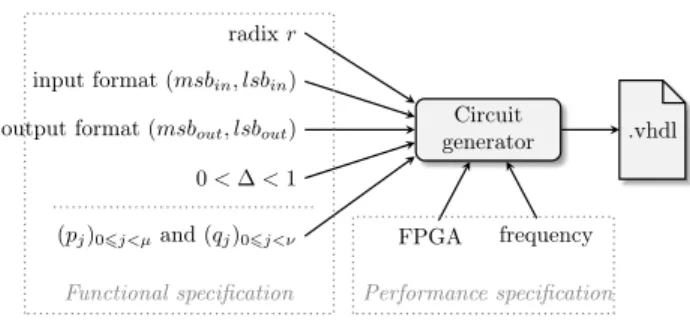
Circuit generator radix 𝑟 input format (𝑚𝑠𝑏𝑖𝑛, 𝑙𝑠𝑏𝑖𝑛) output format (𝑚𝑠𝑏𝑜𝑢𝑡, 𝑙𝑠𝑏𝑜𝑢𝑡) 0 < ∆ < 1
(𝑝𝑗)06𝑗<𝜇and (𝑞𝑗)06𝑗<𝜈 FPGA frequency .vhdl
Functional specification Performance specification
Figure 1: Circuit generator overview. 2.2.2 A solution to a coefficient saturation issue
While we generally obtain integer 𝑎𝑗 and 𝑏𝑗 which correspond to a good approximation, the solution is not always
guaranteed to give a valid simple E-fraction. What happens is that, in many cases, some of the denominator coefficients in 𝑅𝑠 are maximal with respect to the magnitude constraint in (6) (recall that the second line in (6)
can be restated as |𝑞𝑗| 6 𝛼 − max(|𝑎|, |𝑏|)). In this context, the corresponding values of |𝑏𝑗| are usually too large.
We thus propose to fix the problematic values of 𝑏𝑗 to the closest value to the allowable limit that does not break
the E-method magnitude constraints.
The change is minor in (9); we just move the corresponding vectors in the second sum on the left hand side of (9) to the right hand side with opposite sign. The resulting problem can also be solved using the tools from [8,19]. This usually gives a valid simple E-fraction ̂︀𝑅 of very good quality.
2.2.3 Higher radix problems
Coefficient saturation issues get more pronounced by increasing the radix 𝑟. In such cases, care must also be taken with the approximation domain: the |𝑞𝑗| upper magnitude bound 𝛼 − max(|𝑎|, |𝑏|) can become negative,
since 𝛼 = (1 − ∆)/(2𝑟) → 0 as 𝑟 → ∞. To counter this, we use argument and domain scaling ideas presented in [23]. This basically consists in approximating 𝑓 (𝑥) = 𝑓 (2𝑡𝑦), for 𝑦 ∈ [2−𝑡𝑎, 2−𝑡𝑏] as a function in 𝑦. If 𝑡 > 0 is large enough, then the new |𝑞𝑗| bound 𝛼 − max(|2−𝑡𝑎|, |2−𝑡𝑏|) will be > 0.
3
A hardware implementation targeting FPGAs
We now focus on the hardware implementation of the E-method on FPGAs. This section introduces a generator capable of producing circuits that can solve the system A · y = b, through the recurrences of Equations (3)–(5).
The popularity of FPGAs is due to their ability to be reconfigured, and their relevance in prototyping as well as in scientific and high-performance computing. They are composed of large numbers of small look-up tables (LUTs), with 4-6 inputs and 1-2 outputs, and each can store the result of any logic function of their inputs. Any two LUTs on the device can communicate, as they are connected through a programmable interconnect network. Results of computations can be stored in registers, usually two of them being connected to the output of each LUT. These features make of FPGAs a good candidate as a platform for implementing the E-method, as motivated even further below.
3.1
A minimal interface
An overview of the hardware back-end is presented in Figure1. Although not typically accessible to the user, its interface is split between the functional and the performance specification. The former consists of the radix 𝑟, the input and output formats, specified as the weights of their most significant (MSB) and least significant (LSB) bits, the parameter ∆ (input by the user) and the coefficients of the polynomials 𝑃𝜇(𝑥) and 𝑄𝜈(𝑥) (coming from
the rational approximation). Having 𝑚𝑠𝑏𝑖𝑛as a parameter is justified by some of the examples of Section 4,
where even though the input 𝑥 belongs to [−1, 1], the maximum value it is allowed to have is smaller, given by the constraints (6) and (7). This allows for optimizing the datapath sizes. The 𝑚𝑠𝑏𝑜𝑢𝑡 can be computed during
the polynomial/rational approximation phase and passed to the generator.
The circuit generator is developed inside the FloPoCo framework [24], which facilitates the support of classical parameters in the performance specification, such as the target frequency of the circuit, or the target FPGA
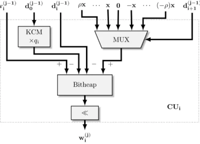
w(j−1)i d(j−1)0 d (j−1) i 𝜌x . . . x 0 −x . . . (−𝜌)x d (j−1) i+1 KCM ×𝑞𝑖 MUX Bitheap ≪ w(j)i + − − + CUi
Figure 2: The basic Computation Unit (CU).
device. It also means that we can leverage on the automatic pipelining and test infrastructure present in the framework, alongside the numerous existing arithmetic operators.
3.2
Implementation details
An overview of the basic iteration, based on Equation (3), is presented in Figure2. As this implementation is targeted towards FPGAs, several optimizations can be applied. First, the multiplication 𝑑(𝑗−1)0 · 𝑞𝑖 can be
computed using the KCM technique for multiplying by a constant [25,26], with the optimizations of [27], that extend the method for real constants. Therefore, instead of using dedicated multiplier blocks (or of generating partial products using LUTs), we can directly tabulate the result of the multiplication 𝑑(𝑗−1)0 · 𝑞𝑖, at the cost of
one LUT per output bit of the result. This remains true even for higher radices, as LUTs on modern devices can accommodate functions of 6 Boolean inputs.
A second optimization relates to the term 𝑑(𝑗−1)𝑖+1 · 𝑥, from Equation (3). Since 𝑑(𝑗−1)𝑖+1 ∈ {−𝜌, . . . , 𝜌}, we can compute the products 𝑥 · 𝜌, 𝑥 · (𝜌 − 1), 𝑥 · (𝜌 − 2), . . . , only once, and then select the relevant one based on the value of 𝑑(𝑗−1)𝑖+1 . The multiplications by the negative values in the digit set come at the cost of just one bitwise operation and an addition, which are combined in the same LUT by the synthesis tools.
Finally, regarding the implementation of the CUs, the multi-operand addition of the terms of Equation (3) is implemented using a bitheap [28]. The alignments of the accumulated terms and their varied sizes would make for a wasteful use of adders. Using a bitheap we have a single, global optimization of the accumulation. In addition, managing sign extensions comes at the cost of a single additional term in the accumulation, using a technique from [10]. The sign extension of a two’s complement fixed point number sxx . . . xx is performed as:
00...0sxxxxxxx + 11...110000000 = ss...ssxxxxxxx
The sum of the constants is computed in advance and added to the accumulation. The final shift comes at just the cost of some routing, since the shift is by a constant amount.
Modern FPGAs contain fast carry chains. Therefore, we represent the components of the residual vector 𝑤 using two’s complement, as opposed to a redundant representation. The selection function uses an estimate of 𝑤𝑖 with one fractional bit allowing a simple tabulation using LUTs.
Iteration 0, the initialization, comes at almost no cost, and can be done through fixed routing in the FPGA. This is also true for the second iteration, as simplifying the equations results in 𝑤(1)𝑖 = 𝑟 ×𝑤(0)𝑖 . The corresponding digits 𝑑(1)𝑖 can be pre-computed and stored directly. This not only saves one iteration, but also improves the accuracy, as 𝑤𝑖(1) and 𝑑(1)𝑖 can be pre-computed using higher-precision calculations. Going one iteration further, we can see that most of the computations required for 𝑤𝑖(2) can also be done in advance, except, of course, those involving 𝑥.
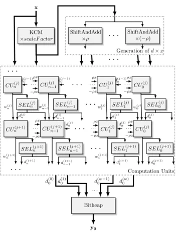
Figure3shows an unrolled implementation of the E-method, that uses the CUs of Figure2 as basic building blocks. At the top of the architecture, a scaling can be applied to the input. This step is optional, and the
x KCM ×𝑠𝑐𝑎𝑙𝑒𝐹 𝑎𝑐𝑡𝑜𝑟 ShiftAndAdd ×𝜌
. . .
ShiftAndAdd ×(−𝜌) Generation of 𝑑 × 𝑥. . .
𝐶𝑈𝑛(𝑗) 𝑆𝐸𝐿(𝑗)𝑛 𝐶𝑈𝑛−1(𝑗) 𝑆𝐸𝐿(𝑗)𝑛−1 . . .. . .
. . .
𝐶𝑈1(𝑗) 𝑆𝐸𝐿(𝑗)1 . . . 𝐶𝑈(𝑗) 0 𝑆𝐸𝐿(𝑗)0 . . . 𝐶𝑈𝑛(𝑗+1) 𝑆𝐸𝐿(𝑗+1)𝑛 𝐶𝑈𝑛−1(𝑗+1) 𝑆𝐸𝐿(𝑗+1)𝑛−1 . . .. . .
. . .
𝐶𝑈1(𝑗) 𝑆𝐸𝐿(𝑗+1)1 . . . 𝐶𝑈(𝑗) 0 𝑆𝐸𝐿(𝑗+1)0 . . .. . .
. . .
Computation Units Bitheap y0 𝑤(𝑗) 𝑛 𝑑(𝑗−1) 0 𝑑(𝑗) 𝑛 𝑤(𝑗) 𝑛−1 𝜌𝑥 −𝜌𝑥 𝑑(𝑗−1) 0 𝑑(𝑖)𝑛−1 𝑤1(𝑗) 𝜌𝑥 −𝜌𝑥 𝑑(𝑗−1) 0 𝑑(𝑗) 1 𝑤0(𝑗) 𝜌𝑥 −𝜌𝑥 𝑑(𝑗) 0 𝑤(𝑗+1) 𝑛 𝑑(𝑖+1) 𝑛 𝜌𝑥 −𝜌𝑥 𝑑(𝑗) 0 𝑑(𝑖+1) 𝑛−1 𝑤(𝑗+1)1 𝜌𝑥 −𝜌𝑥 𝑑(𝑗) 0 𝑑(𝑖+1)1 𝜌𝑥 −𝜌𝑥 𝑑(𝑗+1)0 𝑑(0)0 𝑑 (1) 0 . . . 𝑑(𝑤−1)0 𝑑 (𝑤) 0Figure 3: The E-method circuit generator.
scale factor (optional parameter in the design) can either be set by the user, or computed by the generator so that, given the input format, the parameter ∆ and the coefficients of 𝑃 and 𝑄, the scaled input satisfies the constraints (6) and (7). The multiplications between 𝑥 and the possible values of the digits 𝑑(𝑗)𝑖 are done using the classical shift-and-add technique, a choice justified by the small values of the constants and the small number of bits equal to 1 in their representations. At the bottom of Figure3, the final result 𝑦0 is obtained in two’s
complement representation. Again, this step is also optional, as users might be content with having the result in the redundant representation.
There is one more optimization that can be done here due to an unrolled implementation. Because only the 𝑑(𝑗)0 digits are required to compute 𝑦0, after iteration 𝑚 − 𝑛 we can compute one less element of w(𝑗) and d(𝑗)at
each iteration. This optimization is the most effective when the number of required iterations 𝑚 is comparable to 𝑛, in which case the required hardware is reduced to almost half.
3.3
Error Analysis
To obtain a minimal implementation for the circuit described in Figure3, we need to size the datapaths in a manner that guarantees that the output 𝑦0 remains unchanged, with respect to an ideal implementation, free of
potential rounding errors. To that end, we give an error-analysis, which follows [6, Ch. 2.8]. For the sake of brevity, we focus on the radix 2 case.
In order for the circuit to produce correct results, we must ensure that the rounding errors do not influence the selection function: 𝑆(𝑤̃︀(𝑗)𝑖 ) = 𝑆(𝑤(𝑗)𝑖 ) = 𝑑(𝑗)𝑖 , where the tilded terms represent approximate values. In [6], the idea is to model the rounding errors due to the limited precision used to store the coefficients 𝑝𝑗 and 𝑞𝑗 inside
the matrix 𝐴 as a new error matrix EA= (𝜀𝑖𝑗)𝑛×𝑛. With the method introduced in this paper, the coefficients
are machine representable numbers, and therefore incur no additional error. What remains to deal with are errors due to the limited precision of the involved operators. The only one that could produce rounding errors is the multiplication 𝑑(𝑗−1)0 · 𝑞𝑖. We know that 𝑑
(𝑗−1)
0 > 1 (the case 𝑑 (𝑗−1)
0 = 0 is clearly not a problem), so the LSB
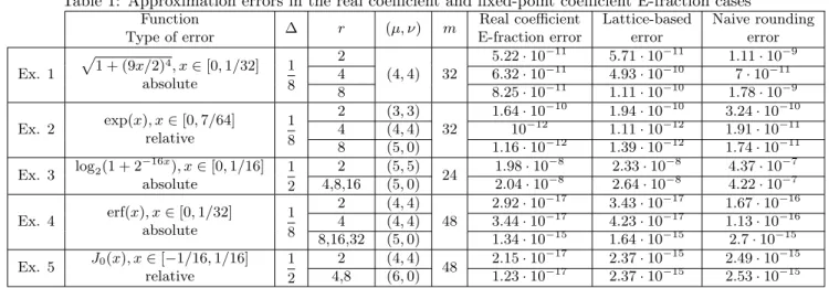
Table 1: Approximation errors in the real coefficient and fixed-point coefficient E-fraction cases Function Type of error Δ 𝑟 (𝜇, 𝜈) 𝑚 Real coefficient E-fraction error Lattice-based error Naive rounding error Ex. 1 √︀1 + (9𝑥/2)4, 𝑥 ∈ [0, 1/32] absolute 1 8 2 (4, 4) 32 5.22 · 10−11 5.71 · 10−11 1.11 · 10−9 4 6.32 · 10−11 4.93 · 10−10 7 · 10−11 8 8.25 · 10−11 1.11 · 10−10 1.78 · 10−9 Ex. 2 exp(𝑥), 𝑥 ∈ [0, 7/64] relative 1 8 2 (3, 3) 32 1.64 · 10−10 1.94 · 10−10 3.24 · 10−10 4 (4, 4) 10−12 1.11 · 10−12 1.91 · 10−11 8 (5, 0) 1.16 · 10−12 1.39 · 10−12 1.74 · 10−11 Ex. 3 log2(1 + 2 −16𝑥 ), 𝑥 ∈ [0, 1/16] absolute 1 2 2 (5, 5) 24 1.98 · 10 −8 2.33 · 10−8 4.37 · 10−7 4,8,16 (5, 0) 2.04 · 10−8 2.64 · 10−8 4.22 · 10−7 Ex. 4 erf(𝑥), 𝑥 ∈ [0, 1/32] absolute 1 8 2 (4, 4) 48 2.92 · 10−17 3.43 · 10−17 1.67 · 10−16 4 (4, 4) 3.44 · 10−17 4.23 · 10−17 1.13 · 10−16 8,16,32 (5, 0) 1.34 · 10−15 1.64 · 10−15 2.7 · 10−15 Ex. 5 𝐽0(𝑥), 𝑥 ∈ [−1/16, 1/16] relative 1 2 2 (4, 4) 48 2.15 · 10 −17 2.37 · 10−15 2.49 · 10−15 4,8 (6, 0) 1.23 · 10−17 2.37 · 10−15 2.53 · 10−15
the case), we perform this operation on its full precision, so we do not require any additional guard bits for the internal computations. If this assumption does not hold, based on [6], we obtain the following expression for the rounding errors introduced when computing w(𝑗) inside Equation (2), denoted with 𝜀(𝑗)w :
𝜀(𝑗)w = 2 · (𝜀(𝑗−1)w + 𝜀𝑐𝑜𝑛𝑠𝑡_𝑚𝑢𝑙𝑡+ EA· d(𝑗−1)).
We can thus obtain an expression for 𝜀(𝑚)w , the error vector at step 𝑚, where 𝑚 is the bitwidth of 𝑦0 and
𝜀𝑐𝑜𝑛𝑠𝑡_𝑚𝑢𝑙𝑡 are the errors due to the constant multipliers. Since 𝜀
(0) w = 0, 𝜀(𝑚)𝑤0 = 2 𝑚· (𝜀 𝑐𝑜𝑛𝑠𝑡_𝑚𝑢𝑙𝑡+ ‖EA‖ · 𝑚 ∑︁ 𝑗=1 𝑑(𝑗)0 · 2−𝑗),
where ‖EA‖ is the matrix 2-norm. We use a larger intermediary precision for the computations, with 𝑔 extra
guard bits. Therefore, we can design a constant multiplier for which 𝜀𝑐𝑜𝑛𝑠𝑡_𝑚𝑢𝑙𝑡6 ¯𝜀𝑐𝑜𝑛𝑠𝑡_𝑚𝑢𝑙𝑡6 2−𝑚−𝑔. Also,
‖EA‖ 6 max 𝑖 𝑛 ∑︁ 𝑗=1 |𝜀𝑖𝑗| and 𝑚 ∑︁ 𝑗=𝑖 𝑑(𝑗)0 · 2−𝑗 < 1,
hence we can deduce that for each 𝑤(𝑚)𝑖 we have 𝜀(𝑚)𝑤𝑖 6 ¯𝜀
(𝑚)
𝑤𝑖 6 2
𝑚(2−𝑚−𝑔+ 𝑛 · 2−𝑚−𝑔). In order for the method
to produce correct results, we need to ensure that ¯𝜀(𝑚)𝑤 6 ∆/2, therefore we need to use 𝑔 > 2 + log2(2(𝑛 + 1)/∆)
additional guard bits. This also takes into consideration the final rounding to the output format.
4
Examples, Implementation and Discussion
In this section, we consider fractions with fixed-point coefficients of 24, 32, and 48 bits: these coefficients will be of the form 𝑖/2𝑚, with −2𝑚
6 𝑖 6 2𝑚, where 𝑤 = 24, 32, 48. The target approximation error in each case is
2−𝑚, i.e., ∼ 5.96 · 10−8, 2.33 · 10−10, 3.55 · 10−15 respectively.
Examples. All the examples are defined in the first column of Table1. When choosing them we considered: ∙ Functions useful in practical applications. The exponential function (Example 2) is a ubiquitous one. Functions of the form log2(1 + 2±𝑘𝑥) (as the one of Example 3) are useful when implementing logarithmic number systems.The erf function (Example 4) is useful in probability and statistics, while the Bessel function 𝐽0 (Example 5) has many applications in physics.
∙ Functions that illustrate the various cases that can occur: polynomials are a better choice (Example 3); rational approximation is better (Examples 1, 2, Example 4 if 𝑟6 8 and Example 5 if 𝑟 = 2). We also include instances where the approximating E-fractions are very different from the minimax, unconstrained, rational approximations with similar degrees in the numerator and denominator (Examples 1 and 2).
All the examples start with a radix 2 implementation after which higher values of 𝑟 are considered. Table1 displays approximation errors in the real coefficient and fixed-point coefficient E-fraction cases. Notice in particular the lattice-based approximation errors, which are generally much better than the naive rounding ones. We also give some complementary comments.
Example 1. The type (4, 4) rational minimax unconstrained approximation error is 4.59 · 10−16, around 5 orders of magnitude smaller than the E-fraction error. A similar difference happens in case of Example 2, where the type (3, 3) unconstrained minimax approximation has error 2.26 · 10−16.
Example 2. In this case, we are actually working with a rescaled input and are equivalently approximating exp(2𝑥), 𝑥 ∈ [0, 7/128]. Also, for 𝑟 = 8, the real coefficient E-fraction is the same as the E-polynomial one (the magnitude constraint for the denominator coefficients is 0).
Example 3. Starting with 𝑟 = 8, we have to scale both the argument 𝑥 and the approximation domain by suitable powers of 2 for the E-method constraints to continue to hold (see end of Section2.1).
Example 4. As with the previous example, for 𝑟 = 16, 32 we have to rescale the argument and interval to get a valid E-polynomial.
Example 5. By a change of variable, we are actually working with 𝐽0(2𝑥 − 1/16), 𝑥 ∈ [0, 1/16]. If we consider
𝑟 > 16, the 48 bits used to represent the coefficients were not sufficient to produce an approximation with error below 2−48.
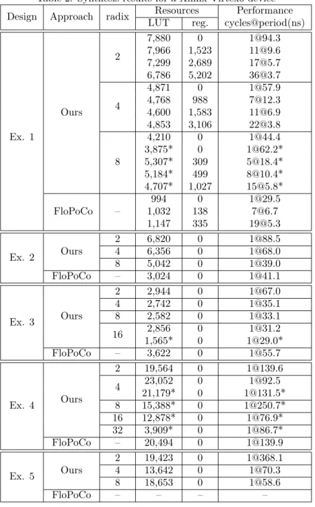
Implementation. We have generated the corresponding circuits for each of the examples, and synthesized them. The target platform is a Xilinx Virtex6 device xc6vcx75t-2-ff484, and the toolchain used is ISE 14.7. The resulting circuit descriptions are in an easily readable and portable VHDL. For each of the examples compare against a state of the art polynomial approximation implementation generated by FloPoCo (described in [9]). FloPoCo [24] is an open-source arithmetic core generator and library for FPGAs. It is, to the best of our knowledge, one of the only alternatives capable of producing the functions chose for comparison. Table2presents the results.
At the top of Table2, for Example 1, we show the flexibility of the generator: it can achieve a wide range of latencies and target frequencies. The examples show how the frequency can be scaled from around 100MHz to 300MHz, at the expense of a deeper pipeline and an increased number of registers. The number of registers approximately doubles each time the circuit’s period is reduced by a factor 2. This very predictable behavior should help the end user make an acceptable trade-off in terms of performance to required resources. The frequency cap of 300MHz is not something inherent to the E-method algorithm, neither to the implementation. Instead it comes from pipeline performance issues of the bitheap framework inside the FloPoCo generator. We expect that once this bottleneck is fixed, our implementations will reach much higher target frequencies, without the need for any modifications in the current implementation.
Discussion. Examples 1 and 2 illustrate that for functions where classical polynomial approximation techniques, like the one used in FloPoCo, manage to find solutions of a reasonably small degree, the ensuing architectures also manage to be highly efficient. This shows, as implementations produced by FloPoCo (with polynomials of degree 6 in both cases) are twice (if not more) as efficient in terms of resources.
However, this is no longer the case when E-fractions can provide a better approximation. This is reflected by Examples 3 to 5, where we obtain a more efficient solution, by quite a large margin in some cases.
For Example 5, Table2does not present any data for the FloPoCo implementation as they do not currently support this type of function.
There are a few remarks to be made regarding the use of a higher radix in the implementations of the E-method. Example 4 is an indication that the overall delay of the architecture reaches a point where it can no longer benefit from increasing the radix. The lines of Table2marked with an asterisk were generated with an alternative implementation for the CUs, which uses multipliers for computing the 𝑑(𝑗−1)𝑖+1 · 𝑥 products. This is due to the exponential increase of the size of multiplexers with the increase of the radix, while the equivalent multiplier only increases linearly. Therefore, there is a crossover point from which it is best to use this version of the architecture, usually at radix 8 or 16. Finally, the effects of truncating the last iterations become the most obvious when the maximum degree 𝑛 is close to the number of required iterations 𝑚 in radix 𝑟. This effect can be observed for Example 3 and 4, where there is a considerable drop in resource consumption between the use of radix 8 and 16, and 16 and 32, respectively.
Table 2: Synthesis results for a Xilinx Virtex6 device Design Approach radix Resources Performance
LUT reg. cycles@period(ns)
Ex. 1 Ours 2 7,880 0 [email protected] 7,966 1,523 [email protected] 7,299 2,689 [email protected] 6,786 5,202 [email protected] 4 4,871 0 [email protected] 4,768 988 [email protected] 4,600 1,583 [email protected] 4,853 3,106 [email protected] 8 4,210 0 [email protected] 3,875* 0 [email protected]* 5,307* 309 [email protected]* 5,184* 499 [email protected]* 4,707* 1,027 [email protected]* FloPoCo – 994 0 [email protected] 1,032 138 [email protected] 1,147 335 [email protected] Ex. 2 Ours 2 6,820 0 [email protected] 4 6,356 0 [email protected] 8 5,042 0 [email protected] FloPoCo – 3,024 0 [email protected] Ex. 3 Ours 2 2,944 0 [email protected] 4 2,742 0 [email protected] 8 2,582 0 [email protected] 16 2,856 0 [email protected] 1,565* 0 [email protected]* FloPoCo – 3,622 0 [email protected] Ex. 4 Ours 2 19,564 0 [email protected] 4 23,052 0 [email protected] 21,179* 0 [email protected]* 8 15,388* 0 [email protected]* 16 12,878* 0 [email protected]* 32 3,909* 0 [email protected]* FloPoCo – 20,494 0 [email protected] Ex. 5 Ours 2 19,423 0 [email protected] 4 13,642 0 [email protected] 8 18,653 0 [email protected] FloPoCo – – – –
5
Summary and Conclusions
A high throughput system for the evaluation of functions by polynomials or rational functions using simple and uniform hardware is presented. The evaluation is performed using the unfolded version of the E-method, with a latency proportional to the precision. An effective computation of the coefficients of the approximations is given and the best strategies (choice of polynomial vs rational approximation, radix of the iterations) investigated. Designs using a circuit generator for the E-method inside the FloPoCo framework are developed and implemented using FPGAs for five different functions of practical interest, using various radices. As it stands, and as our examples show for FPGA devices, the E-method is generally more efficient as soon as the rational approximation is significantly more efficient than the polynomial one. From a hardware standpoint, the results show it is desirable to use the E-method with high radices, usually at least 8. The method also becomes efficient when we manage to find a balance between the maximum degree 𝑛 of the polynomial or E-fraction and the number of iterations required for converging to a correct result, which we can control by varying the radix. An open-source implementation of our approach will soon be available online at https://github.com/sfilip/emethod.
Acknowledgments
This work was partly supported by the FastRelax project of the French Agence Nationale de la Recherche, EPSRC (UK) under grants EP/K034448/1 and EP/P010040/1, the Royal Academy of Engineering and Imagination Technologies.
A
Convergence of the E-fraction differential correction algorithm
The E-fraction approximation problem can be formulated in terms of finding functions of the form
𝑅(𝑥) = 𝑃 (𝑥)/𝑄(𝑥) := ∑︀𝜇
𝑗=0𝛼𝑗𝑥 𝑗
1 +∑︀𝜈𝑗=1𝛽𝑗𝑥𝑗, (10)
that best approximate 𝑓 , where the denominator coefficients are bounded in magnitude, i.e., max
16𝑘6𝜈|𝛽𝑘| 6 𝑑 > 0, (11)
and 𝑄(𝑥) > 0, ∀𝑥 ∈ 𝑋. We denote this set as ℛ𝜇,𝜈(𝑋). In this case, the differential correction algorithm is defined as follows: given 𝑅𝑘= 𝑃𝑘/𝑄𝑘∈ ℛ𝜇,𝜈(𝑋) satisfying (10) and (11), find 𝑅 = 𝑃/𝑄 that minimizes the expression
max 𝑥∈𝑋 {︂ |𝑓 (𝑥)𝑄(𝑥) − 𝑃 (𝑥)| − 𝛿𝑘𝑄(𝑥) 𝑄𝑘(𝑥) }︂ , subject to max 16𝑘6𝜈|𝛽𝑗| 6 𝑑,
where 𝛿𝑘= max𝑥∈𝑋|𝑓 (𝑥) − 𝑅𝑘(𝑥)|. If 𝑅 = 𝑃/𝑄 is not good enough, continue with 𝑅𝑘+1= 𝑅.
The convergence properties of this variation are similar to those of the original differential correction algorithm. Let 𝛿*= inf𝑅∈ℛ𝜇,𝜈(𝑋)‖𝑓 − 𝑅‖, where ‖𝑔‖ = max𝑥∈𝑋|𝑔(𝑥)|.
Theorem 1. If 𝑄𝑘(𝑥) > 0, ∀𝑥 ∈ 𝑋 and if 𝛿𝑘̸= 𝛿, then 𝛿𝑘+1< 𝛿𝑘 and 𝑄𝑘+1(𝑥) > 0, ∀𝑥 ∈ 𝑋. Proof. Since 𝛿𝑘̸= 𝛿*
, there exists 𝑅 = 𝑃 /𝑄 ∈ ℛ𝜇,𝜈(𝑋) s.t. ‖𝑓 − 𝑅‖ = 𝛿 < 𝛿𝑘. Let Δ = min𝑥∈𝑋⃒⃒𝑄(𝑥)⃒⃒and 𝑀 = 1 + 𝑑 max𝑥∈𝑋
∑︀𝜈 𝑘=1
⃒
⃒𝑥𝑘⃒⃒so that |𝑄(𝑥)|6 𝑀 over 𝑋 for any rational function satisfying (10) and (11). By the definition of 𝑃𝑘+1and 𝑄𝑘+1, we have
max𝑥∈𝑋{︂ |𝑓 (𝑥)𝑄𝑘+1(𝑥) − 𝑃𝑘+1(𝑥)| − 𝛿𝑘𝑄𝑘+1(𝑥) 𝑄𝑘(𝑥) }︂ 6 max𝑥∈𝑋 {︃ ⃒ ⃒𝑓 (𝑥)𝑄(𝑥) − 𝑃 (𝑥)⃒⃒− 𝛿𝑘𝑄(𝑥) 𝑄𝑘(𝑥) }︃ 6 max𝑥∈𝑋 {︂[︂⃒ ⃒ ⃒ ⃒ 𝑓 (𝑥) −𝑃 (𝑥) 𝑄(𝑥) ⃒ ⃒ ⃒ ⃒ − 𝛿𝑘 ]︂ 𝑄(𝑥) 𝑄𝑘(𝑥) }︂ 6 max𝑥∈𝑋 {︂ (𝛿 − 𝛿𝑘) 𝑄(𝑥) 𝑄𝑘(𝑥) }︂ = −(𝛿𝑘− 𝛿) min𝑥∈𝑋 𝑄(𝑥) 𝑄𝑘(𝑥) 6 −Δ 𝑀(𝛿𝑘− 𝛿). This chain of inequalities tells us that
𝛿𝑘𝑄𝑘+1(𝑥)/𝑄𝑘(𝑥) > Δ(𝛿𝑘− 𝛿)/𝑀, ∀𝑥 ∈ 𝑋 (12)
resulting in 𝑄𝑘+1(𝑥) > 0, ∀𝑥 ∈ 𝑋 and
{|𝑓 (𝑥)𝑄𝑘+1(𝑥) − 𝑃𝑘+1(𝑥)| − 𝛿𝑘𝑄𝑘+1(𝑥)} /𝑄𝑘(𝑥) < 0, ∀𝑥 ∈ 𝑋, leading to
|𝑓 (𝑥) − 𝑃𝑘+1(𝑥)/𝑄𝑘+1(𝑥)| < 𝛿𝑘, ∀𝑥 ∈ 𝑋. The conclusion now follows by the definition of 𝛿𝑘.
Theorem 2.
𝛿𝑘→ 𝛿*as 𝑘 → ∞.
Proof. By the previous theorem, we know that {𝛿𝑘} is a monotonically decreasing sequence bounded below by 0. It is thus convergent. Denote its limit by 𝛿 and assume that 𝛿 > 𝛿*. Then, there exists 𝑅 = 𝑃 /𝑄 ∈ ℛ𝜇,𝜈(𝑋) s.t.
⃦
⃦𝑓 − 𝑅⃦⃦= 𝛿 < 𝛿.
Let Δ and 𝑀 be as in the previous theorem. By the aforementioned chain of inequalities, we get ⃒ ⃒ ⃒ ⃒ 𝑓 (𝑥) −𝑃𝑘+1(𝑥) 𝑄𝑘+1(𝑥) ⃒ ⃒ ⃒ ⃒ − 𝛿𝑘6 −Δ 𝑀(𝛿𝑘− 𝛿) 𝑄𝑘(𝑥) 𝑄𝑘+1(𝑥), ∀𝑥 ∈ 𝑋 and 𝛿𝑘+1− 𝛿𝑘6 −Δ 𝑀(𝛿𝑘− 𝛿) 𝑄𝑘(𝑧𝑘) 𝑄𝑘+1(𝑧𝑘), (13)
where 𝑧𝑘 is an element of 𝑋 minimizing 𝑄𝑘(𝑥)
𝑄𝑘+1(𝑥). Since 𝛿𝑘converges to 𝛿 > 𝛿, (13) implies that
lim 𝑘→∞ 𝑄𝑘(𝑧𝑘) 𝑄𝑘+1(𝑧𝑘) = 0. (14) From (12) we get 𝑄𝑘+1(𝑥) > 𝑄𝑘(𝑥)Δ 𝑀(𝛿𝑘− 𝛿)/𝛿𝑘> 𝑐𝑄𝑘(𝑥), ∀𝑥 ∈ 𝑋, (15) provided that 𝑐6 Δ 𝑀(1 − 𝛿/𝛿) 6 Δ 𝑀(𝛿𝑘− 𝛿)/𝛿𝑘. Taking 𝑐 = min{︂ 1 2, Δ 𝑀(1 − 𝛿/𝛿) }︂ ,
it follows from (14) that there exists a positive integer 𝑘0 such that 𝑄𝑘(𝑧𝑘)
𝑄𝑘+1(𝑧𝑘) 6 𝑐 |𝑋|
Using (15) and (16), we have 𝑄𝑘(𝑧𝑘) 𝑄𝑘+1(𝑧𝑘) ∏︁ 𝑥∈𝑋,𝑥̸=𝑧𝑘 𝑄𝑘(𝑥) 𝑄𝑘+1(𝑥)6 𝑐 |𝑋|(︂ 1 𝑐 )︂|𝑋|−1 = 𝑐, and ∏︁ 𝑥∈𝑋 𝑄𝑘+1(𝑥) 𝑄𝑘(𝑥) > 1 𝑐 > 2. It follows that∏︀
𝑥∈𝑋𝑄𝑘(𝑥) diverges as 𝑘 → ∞. This contradicts the normalization condition (11).
References
[1] J. E. Volder, “The CORDIC computing technique,” IRE Transactions on Electronic Computers, vol. EC-8, no. 3, pp. 330–334, 1959, reprinted in E. E. Swartzlander, Computer Arithmetic, Vol. 1, IEEE Computer Society Press, Los Alamitos, CA, 1990.
[2] W. F. Wong and E. Goto, “Fast hardware-based algorithms for elementary function computations using rectangular multipliers,” IEEE Trans. Comput., vol. 43, no. 3, pp. 278–294, Mar. 1994.
[3] D. D. Sarma and D. W. Matula, “Faithful bipartite ROM reciprocal tables,” in Proceedings of the 12th IEEE Symposium on Computer Arithmetic (ARITH-12), Knowles and McAllister, Eds. IEEE Computer Society Press, Los Alamitos, CA, Jun. 1995, pp. 17–28.
[4] M. J. Schulte and J. E. Stine, “Approximating elementary functions with symmetric bipartite tables,” IEEE Trans. Comput., vol. 48, no. 8, pp. 842–847, Aug. 1999.
[5] F. de Dinechin and A. Tisserand, “Multipartite table methods,” IEEE Trans. Comput., vol. 54, no. 3, pp. 319–330, Mar. 2005.
[6] M. D. Ercegovac, “A general method for evaluation of functions and computation in a digital computer,” Ph.D. dissertation, Dept. of Computer Science, University of Illinois, Urbana-Champaign, IL, 1975.
[7] ——, “A general hardware-oriented method for evaluation of functions and computations in a digital computer,” IEEE Trans. Comput., vol. C-26, no. 7, pp. 667–680, 1977.
[8] N. Brisebarre, S. Chevillard, M. D. Ercegovac, J.-M. Muller, and S. Torres, “An Efficient Method for Evaluating Polynomial and Rational Function Approximations,” in 19th IEEE Conference on Application-specific Systems, Architectures and Processors. ASAP’2008, Leuven (Belgium), 2–4 July 2008, pp. 233–238.
[9] F. de Dinechin, “On fixed-point hardware polynomials,” Tech. Rep., Oct. 2015, working paper or preprint. [Online]. Available: https://hal.inria.fr/hal-01214739
[10] M. D. Ercegovac and T. Lang, Digital Arithmetic. Morgan Kaufmann Publishers, San Francisco, CA, 2004. [11] E. W. Cheney, Introduction to Approximation Theory, 2nd ed. AMS Chelsea Publishing. Providence, RI, 1982. [12] M. J. D. Powell, Approximation theory and methods. Cambridge University Press, 1981.
[13] R. Reemtsen, “Modifications of the first Remez algorithm,” SIAM J. Numer. Anal., vol. 27, no. 2, pp. 507–518, 1990. [14] E. W. Cheney and H. L. Loeb, “Two new algorithms for rational approximation,” Numer. Math., vol. 3, no. 1, pp.
72–75, 1961.
[15] S. N. Dua and H. L. Loeb, “Further remarks on the differential correction algorithm,” SIAM J. Numer. Anal., vol. 10, no. 1, pp. 123–126, 1973.
[16] I. Barrodale, M. J. D. Powell, and F. K. Roberts, “The differential correction algorithm for rational ℓ∞-approximation,” SIAM J. Numer. Anal., vol. 9, no. 3, pp. 493–504, 1972.
[17] D. Dudgeon, “Recursive filter design using differential correction,” IEEE Trans. Acoust., Speech, Signal Process., vol. 22, no. 6, pp. 443–448, 1974.
[18] J.-M. Muller, N. Brisebarre, F. de Dinechin, C.-P. Jeannerod, V. Lefèvre, G. Melquiond, N. Revol, D. Stehlé, and S. Torres,Handbook of Floating-Point Arithmetic. Birkhäuser, 2010.
[19] N. Brisebarre and S. Chevillard, “Efficient polynomial 𝐿∞ approximations,” in ARITH ’07: Proceedings of the 18th IEEE Symposium on Computer Arithmetic, Montpellier, France. IEEE Computer Society, 2007, pp. 169–176. [20] P. Q. Nguyen and B. Vallée, Eds., The LLL Algorithm - Survey and Applications, ser. Information Security and
Cryptography. Springer, 2010. [Online]. Available: http://dx.doi.org/10.1007/978-3-642-02295-1
[21] A. K. Lenstra, H. W. Lenstra, and L. Lovász, “Factoring polynomials with rational coefficients,” Math. Ann., vol. 261, no. 4, pp. 515–534, 1982.
[22] L. Babai, “On Lovász’ lattice reduction and the nearest lattice point problem,” Combinatorica, vol. 6, no. 1, pp. 1–13, 1986.
[23] N. Brisebarre and J.-M. Muller, “Functions approximable by E-fractions,” in Proc. 38th Asilomar Conference on Signals, Systems and Computers, Nov. 2004.
[24] F. de Dinechin and B. Pasca, “Designing custom arithmetic data paths with FloPoCo,” IEEE Des. Test Comput., vol. 28, no. 4, pp. 18–27, Jul. 2011.
[25] K. Chapman, “Fast integer multipliers fit in FPGAs (EDN 1993 design idea winner),” EDN magazine, no. 10, p. 80, May 1993.
[26] M. J. Wirthlin, “Constant coefficient multiplication using look-up tables,” VLSI Signal Processing, vol. 36, no. 1, pp. 7–15, 2004.
[27] A. Volkova, M. Istoan, F. De Dinechin, and T. Hilaire, “Towards Hardware IIR Filters Computing Just Right: Direct Form I Case Study,” Tech. Rep., 2017. [Online]. Available: http://hal.upmc.fr/hal-01561052/
[28] N. Brunie, F. de Dinechin, M. Istoan, G. Sergent, K. Illyes, and B. Popa, “Arithmetic core generation using bit heaps,” in Proceedings of the 23rd Conference on Field-Programmable Logic and Applications, Sep. 2013, pp. 1–8.