HAL Id: hal-00707510
https://hal.archives-ouvertes.fr/hal-00707510
Submitted on 12 Jun 2012
HAL is a multi-disciplinary open access
archive for the deposit and dissemination of
sci-entific research documents, whether they are
pub-lished or not. The documents may come from
teaching and research institutions in France or
abroad, or from public or private research centers.
L’archive ouverte pluridisciplinaire HAL, est
destinée au dépôt et à la diffusion de documents
scientifiques de niveau recherche, publiés ou non,
émanant des établissements d’enseignement et de
recherche français ou étrangers, des laboratoires
publics ou privés.
Improving the Asymmetric TSP by Considering Graph
Structure
Jean-Guillaume Fages, Xavier Lorca
To cite this version:
Jean-Guillaume Fages, Xavier Lorca. Improving the Asymmetric TSP by Considering Graph
Struc-ture. 2012. �hal-00707510�
Improving the Asymmetric TSP
by Considering Graph Structure
Jean-Guillaume Fages and Xavier Lorca
June 9, 2012 ´
Ecole des Mines de Nantes, LINA UMR CNRS 6241, FR-44307 Nantes Cedex 3, France
{Jean-Guillaume.Fages,Xavier.Lorca}@mines-nantes.fr
Abstract. Recent works on cost based relaxations have improved Con-straint Programming (CP) models for the Traveling Salesman Problem (TSP). We provide a short survey over solving asymmetric TSP with CP. Then, we suggest new implied propagators based on general graph properties. We experimentally show that such implied propagators bring robustness to pathological instances and highlight the fact that graph structure can significantly improve search heuristics behavior. Finally, we show that our approach outperforms current state of the art results.
1
Introduction
Given a n node, m arc complete directed weighted graph G = (V, A, f : A → R), the Asymmetric Traveling Salesman Problem [1] (ATSP) consists in finding a partial subgraph G0 = (V, A0, f ) of G which forms a Hamiltonian circuit of min-imum cost. This NP-hard problem is one of the most studied by the Operation Research community. It has various practical applications such as vehicle routing problems of logistics, microchips production optimization or even scheduling.
The symmetric TSP is well handled by linear programming techniques [1]. However, such methods suffer from the addition of side constraints and asymmet-ric cost matrix, whereas constraint programming models do not. Since the real world is not symmetric and industrial application often involve constraints such as time windows, precedences, loading capacities and several other constraints, improving the CP general model for solving the ATSP leads to make CP more competitive on real world routing problems. Recent improvements on cost based relaxations [4] had a very strong impact on the ability of CP technologies to solve the TSP. In this paper, we investigate how the graph structure can contribute to the resolution process, in order to tackle larger instances. For this purpose, we developed usual and original filtering algorithms using classical graph struc-tures, such as strongly connected components or dominators. We analyzed their behavior both from a quantitative (time complexity) and a qualitative (con-sistency level) point of view. Also, we experimentally show that such implied propagators bring robustness to hard instances, and highlight the fact that the
graph structure can significantly improve the behavior of search heuristics. Our main contribution is both a theoretical and an experimental study which lead to a robust model that outperforms state of the art results in CP.
This paper is divided into six main parts. Section 2 provides some vocabulary and notations. Section 3 discusses the state of the art implied constraints. Next, we show in Section 4 how the reduced graph can provide useful information for pruning and improving existing models. In Section 5 we provide some improve-ments about the implementation of the Held and Karp method within a directed context. Section 6 shows an experimental study on the ATSP and some openings about its symmetric version (TSP). Section 7 concludes the paper with several perspectives.
2
Background
Let us consider a directed graph G = (V, A). A Strongly Connected Component (SCC) is a maximal subgraph of G such that for each pair of nodes {a, b} ∈ V2,
a path exists from a to b and from b to a. A reduced graph GR= (VR, AR) of a
directed graph G represents the SCC of G. This graph is obtained by merging the nodes of G which are in the same SCC and removing any loop. Such a graph is unique and contains no circuit. We link G and GR with two functions:
sccOf : V → VRand nodesOf : VR→ VV. The method sccOf can be represented
by one n-size integer array. Also, since each node of V belongs to exactly one SCC of VR, the method nodesOf can be represented by two integer arrays: the
first one represents the canonical element of each SCC while the second one links nodes of the same SCC, behaving like a linked list. Those two arrays have respectively size of nR and n, where nR = |VR|. The transitive closure of G
is a graph GT C = (V, AT C) representing node reachability in G, i.e. such that
(i, j) ∈ AT C if and only if a path from i to j exists in G.
In a CP context a Graph Variable can be used to model a graph. Such a concept has been introduced by Le Pape et al. [24] and detailed by R´egin [28] and Dooms et al. [9]. We define a graph variable GV by two graphs: the graph of potential elements, GP = (VP, AP), contains all the nodes and arcs
that potentially occur in at least one solution whereas the graph of mandatory elements, GM = (VM, AM), contains all the nodes and arcs that occur in every
solution. It has to be noticed that GM ⊆ GP ⊆ G. During resolution, decisions
and filtering rules will remove nodes/arcs from GP and add nodes/arcs to GM
until the Graph Variable is instantiated, i.e. when GP = GM. It should be
noticed that, regarding the TSP, VP = VM = V , so resolution will focus on AM
and AP: branching strategies and propagators will remove infeasible arcs from
3
Related Work
This section describes the state of the art of existing approaches for solving ATSP with CP. We distinguish the structural filtering, which ensures that a solution is a Hamiltonian path, from cost based pruning, which mainly focus on the solution cost. Then, we study a few representative branching heuristics.
Given, a directed weighted graph G = (V, A, f ), and a function f : A → R, the ATSP consists in finding a partial subgraph G0= (V, A0, f ) of G which forms
a Hamiltonian circuit of minimum cost. A simple ATSP model in CP, involving a graph variable GV , can basically be stated as minimizing the sum of costs of arcs in the domain of GV and maintaining GV to be a Hamiltonian circuit with a connectivity constraint and a degree constraint (one predecessor and one successor for each node). However, it is often more interesting to convert such a model in order to find a path instead of a circuit [15, 25]. Our motivation for this transformation is that it brings graph structure that is more likely to be exploited.
In this paper, we consider the ATSP as the problem of finding a minimum cost Hamiltonian path with fixed start and end nodes in a directed weighted graph. In the following, s, e ∈ V respectively denote the start and the end of the expected path. s and e are supposed to be known. They can be obtained by duplicating any arbitrary node, but it makes more sense to duplicate the node representing the salesman’s home.
3.1 Structural filtering algorithms
Our formulation of the ATSP involves the search of a path instead of a circuit, the degree constraints has thus to be stated as follows: For all v ∈ V \{e}, δG+0(v) = 1 and for any v ∈ V \{s}, δG−0(v) = 1, where δ+G0(v) (respectively δ−G0(v)) denotes the number of successors (respectively predecessors) of v. Extremal conditions, being δG+0(e) = δ−G0(s) = 0, are ensured by the initial domain of the graph vari-able. An efficient filtering can be obtained with two special purpose incremental propagators. One reacts on mandatory arc detections: whenever arc (u, v) is en-forced, other outgoing arc of u and ingoing arcs of v can be pruned. The other reacts on arc removals: whenever a node has only one outgoing (or ingoing) potential arc left, this arc is mandatory and can be enforced. A higher level of consistency can be achieved by using a graph-based AllDifferent constraint maintaining a node-successor perfect matching [27]. Deleting circuits is the sec-ond important structural aspect of the TSP. Caseau and Laburthe [7] suggested the simple and efficient NoCycle constraint to remove circuits of the graph. Their fast incremental algorithm is based on the subpaths fusion process. It runs in constant time per arc enforcing event. The conjunction of this circuit elimination constraint and the above degree constraints is sufficient to guarantee that the solution is a Hamiltonian path from s to e.
However, other implied constraints provide additional filtering that may help the resolution process. For instance, Quesada [26] suggested the general propaga-tor DomReachability which maintains the transitive closure and the dominance
tree of the graph variable. However, its running time, O(nm) in the worst case, makes it unlikely to be profitable in practice. A faster constraint, also based on the concept of dominance, is the Arborescence constraint. It is nothing else but a simplification of the Tree constraint [2] recently improved to a O(n + m) worst case time complexity [12]. Given a graph variable GV and a node s, such a con-straint ensures that GV is an arborescence rooted in node s. More precisely, it enforces GAC over the conjunction of the following properties: GPhas no circuit,
each node is reachable from s and, each node but s has exactly one predecessor. Such a filtering can also be used to define the AntiArborescence by switching s with e and predecessors with successors.
A dual approach consists in assigning to each node its position in the path. In such a case, the position of a node is represented by an integer variable with initial domain [0, n − 1]. Positions are different from a node to another, which can be ensured by an AllDifferent constraint. Since the number of nodes is equal to the number of positions, the bound consistency algorithm of AllDifferent constraint only requires O(n) time. Plus, a channeling has to be done between the graph variable and position variables. Such a channeling requires O(n + m) worst case time. In particular, lower bounds of positions are adjusted according to a single Breadth First Search (BFS) of GP(s) while upper
bounds of positions are shortened by a BFS of G−1P (e). It has to be noticed that this approach is related to disjunctive scheduling [33]: nodes are tasks of duration 1 which are executed on the same machine. The structure of the input graph creates implicit precedence constraints.
Finally, some greedy procedures based on the finding of cuts have been sug-gested in the literature: Benchimol et al. enforce some cut-sets of size two [4] while Kaya and Hooker use graph separators for pruning [21]. The drawback of such methods is that they provide no level of consistency.
3.2 Cost-based filtering algorithms
CP models often embed relaxation based constraints, to provide inference from costs. Fischetti and Toth [14] suggested a general bounding procedure for com-bining different relaxations of the same problem.
The most natural relaxation is obtained by considering the cheapest outgoing arc of each node: LBtrivial =Pu∈V \{e}min{f (u, v)|(u, v) ∈ AP}. Such a lower
bound can be computed efficiently but it is in general relatively far from the optimal value.
A stronger relaxation is the weighted version of the AllDifferent con-straint, corresponding to the Minimum Assignment Problem (MAP). It requires O(n(m + n log n)) time [23] to compute a first minimum cost assignment but then O(n2) time [6] to check consistency and filter incrementally. Some
inter-esting evaluations are provided by [16], but are mainly related to the TSP with time windows constraints.
A widely exploited subproblem of the ATSP is the Minimum Spanning Tree (MST) problem where the degree constraint and arc direction are relaxed. We remark that a hamiltonian path is a spanning tree and that it is possible to
compute a MST with a degree restriction at one node [17]. A MST can be computed in two ways. The first one is Kruskal’s algorithm, which runs in O(αm) worst case time, where α is the inverse Ackermann function, but re-quires edges to be sorted according to their weights. Sorting edges can be done once and for all in O(m log m) time. The second option is to use Prim’s algo-rithm which requires O(m+n log n) time with Fibonacci heaps [17] or O(m log n) time if binomial heaps are used instead. Based on Kruskal’s algorithm, R´egin et al. [29, 30] made the Weighted Spanning Tree constraint which ensures con-sistency, provides a complete pruning and detects mandatory arcs incremen-tally, within O(αm) time. Dooms and Katriel [10, 11] presented a more complex Minimum Spanning Tree constraint which maintains a graph and its spanning tree, pruning according to King’s algorithm [22].
An improvement of the MST relaxation is the approach of Held and Karp [19], adapted for CP by Benchimol et al.[4]. It is the Lagrangian MST relaxation with a policy for updating Langrangian multipliers that provides a fast convergence. The idea of this method is to iteratively compute MST that converge towards a path by adding penalties on arc costs according to degree constraints violations. It must be noticed that since arc costs change from one iteration to another, Prim’s algorithm is better than Kruskal’s which requires to sort edges. Moreover, to our knowledge neither algorithm can be applied incrementally.
A more accurate relaxation is the Minimum Spanning Arborescence (MSA) relaxation, since it does not relax the orientation of the graph. This relaxation has been studied by [14, 15] who provide a O(n2) time filtering algorithm based
on primal/dual linear programs. The best algorithm for computing a MSA has been provided by Gabow et al. [17]. Their algorithm runs in O(m+n log n) worst case time, but it does not provide reduced costs that are used for pruning. Thus, it could be used to create a Minimum Spanning Arborescence constraint with a O(m + n log n) time consistency checking but the complete filtering algorithm remains in O(n2) time. The Lagrangian MSA relaxation, with a MSA computa-tion based on Edmonds’ algorithm, has been suggested in [7]. This method was very accurate but unfortunately unstable. Also, Benchimol et al. [4] report that the MSA based Held and Karp scheme lead to disappointing results.
3.3 Branching heuristics
Branching strategies forms a fundamental aspect of CP which can drastically re-duce the search space. We study here dedicated heuristics, because the literature is not clear about which branching heuristic should be used.
Pesant et al. have introduced Sparse heuristic [25] which has the singularity of considering occurrences of successors and ignoring costs. In this way, this heuris-tic is based on the graph structure. It behaves as following: First, it selects the set of nodes X with no successor in GM and the smallest set of successors in GP.
Sec-ond, it finds the node x ∈ X which maximizeP
(x,y)∈AP|{(z, y) ∈ AP|z ∈ X}|. The heuristic then iterates on x’s successors. This process is optimized by per-forming a dichotomic exploration of large domains.
However, very recently, Benchimol et al. [4] suggested a binary heuristic, based on the MST relaxation, that we call RemoveMaxRC. It consists in remov-ing from GP the tree arc of maximum replacement cost, i.e. the arc which would
involve the highest cost augmentation if it was removed. By tree arc, we mean the fact that it appears in the MST of the last iteration of the Held and Karp procedure. Acutally, as shown in section 6, this branching leads to poor results and should not be used.
Finally, Focacci et al. solve the TSPTW [15] by guiding the search with time windows, which means that the efficiency of CP for solving the ATSP should not rely entirely on its branching heuristic.
4
Considering the reduced graph
In this section, we consider a subproblem which is not a subset of constraints, as usual, but consists in the whole ATSP itself applied to a more restrictive scope: the reduced graph of GP. The structure of the reduced graph has already been
considered in a similar way for path partitioning problems [3, 5]. In this sec-tion, we first study structural properties that arise from considering the reduced graph. Second, we show how to adapt such information to some state of the art implied models, including cost based reasonings.
4.1 Structural properties
We introduce a propagator, the Reduced Path propagator, which makes the reduced graph a (Hamiltonian) simple path and ensures by the way that each node is reachable from s and can reach e. It is a monotonic generalization of the algorithm depicted in [31]. Necessary conditions for this propagator have already been partially highlighted in [5]. We first modify them in order to fit with the TSP and our model. Next, we provide a linear time incremental algorithm. Definition 1. Reduced path guarantees that any arc in GP that connects two
SCC, is part of a simple path which go through every SCC of GP.
Proposition 1. Given any directed graph G, its reduced graph GR contains at
most one Hamiltonian path.
Proof. Let us consider a graph G such that GRcontains at least two Hamiltonian
paths p1 and p2, p1 6= p2. Since both p1 and p2 are Hamiltonian then there exists at least two nodes {x, y} ⊂ VR, x 6= y, such that x is visited before y in p1 and
after y in p2. Thus, the graph P = p1S p2 contains a path from x to y and from y to x. This is a circuit. As P ⊂ GR, GR also contains a circuit, which is
a contradiction. ut
We note GR the reduced graph of GP. We remark that, as s has no
pre-decessor then its SCC is the node s itself. Also, as e has no successor then sccOf(e)= {e}. To distinguish nodes of V from nodes of the reduced graph, we note sccOf(s)= sRand sccOf(e)= eR. It follows that any Hamiltonian path in
Proposition 2. If there exists a Hamiltonian path from s to e in GP then there
exists a Hamiltonian path in GR.
Proof. Lets suppose that GR has no Hamiltonian path from sRto eR. Then for
any path pRin GRstarting at sRand ending at eR, there exist at least one node
x ∈ VR, which is not visited by pR. Thus, for any path pE in GP starting at s
and ending at e, there exist at least one SCC x ∈ VR which is not traversed by
pE, so ∀u ∈ nodesOf(x ), then u /∈ pE. Thus any path in GP starting at s and
ending at e is not Hamiltonian. ut It follows that any transitive arc of GR must be pruned and that remaining
arcs of GRare mandatory (otherwise the graph becomes disconnected): any SCC,
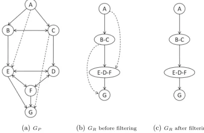
but eR, must have exactly one outgoing arc. An example is given in figure 1:
the graph GP contains four SCC. Its reduced graph, GR, has a unique
Hamilto-nian path PR= ({A}, {B, C}, {E, D, F }, {G}). Arcs of GR\PR are infeasible so
(A, E) and (C, G) must be pruned from GP.
(a)GP (b)GRbefore filtering (c)GRafter filtering
Fig. 1. Reduced Path filtering, transitive arcs (dotted) are infeasible.
We introduce a new data structure in GR that we call outArcs : for each
node x ∈ VR, outArcs(x ) is the list of arcs {(u, v) ∈ AP| sccOf(u)= x and
sccOf(v )6= x}. We can now easily draw a complete filtering algorithm for the Reduced Path propagator which ensures the GAC over the property that GR
must be a path in O(n + m) time:
1. Data structures: Compute the SCC of GP (with Tarjan’s algorithm [32]) and
build the reduced graph GR= (VR, AR).
2. Taking mandatory arcs into account: ∀(u, v) ∈ AM such that x =sccOf(u)
3. Consistency checking: Make GRa path if possible, fail otherwise.
4. for each arc (u, v) ∈ AP such that x =sccOf(u) and y =sccOf(v ), x 6= y,
(a) Pruning: if (x, y) /∈ AR, remove arc (u, v).
(b) Enforcing: if (x, y) ∈ AR and (u, v) is the only arc of AP that links x
and y, enforce arc (u, v).
A procedure performing step 3 starts on node sR, finds its right successor next
(the one which has only one predecessor) and removes other outgoing arcs. Then, the same procedure is applied on next and so on, until eR is reached. Such an
algorithm must be performed once during the initial propagation. Then, the propagator reacts to fine events. To have an incremental behavior, the propagator must maintain the set of SCC and the reduced graph. Haeupler et al. [18] worked on maintaining SCC and a topological ordering of nodes in the reduced graph, but under the addition of arcs. We deal with arc deletions. Moreover, we may have lots of arc deletions per propagation (at least for the first ones), thus we should not use a completely on-line algorithm.
SCC maintenance: Let us consider an arc (u, v) ∈ AP such that sccOf(u)= x
and sccOf(v )= y. If x 6= y and if (u, v) is removed from AP then it must be
removed from outArcs(x ) also. If x = y then the removal of (u, v) may split the SCC x, so computation is required. As many arcs can be removed from one prop-agation to another, we suggest a partially incremental algorithm which computes exclusively SCC that contains at least one removed arc, each one exactly once. We introduce a bit set to mark nodes of GR. Initially, each node is unmarked,
then when a removed arc, inside an unmarked SCC x, is considered, we apply Tarjan’s algorithm on GPT nodesOf(x ) and mark x. Tarjan’s algorithm will
return either x if x is still strongly connected, or the new set of SCC induced by all arc removals from x. In both cases, we can ignore other arcs that have been removed from nodesOf(x ). Since the SCC of a graph are node-disjoint, the overall processing time of a propagation dealing with k arc deletions involving some SCC K ⊂ VR isPx∈KO(nx+ mx) = O(n + m).
GR maintenance and filtering: Algorithm 1 shows how to get an incremental
propagator that reacts to SCC splits. When a SCC x is split into k new SCC, the reduced graph gets k − 1 new nodes and must be turned into a path while some filtering may be performed on GV . The good thing is that there is no need to consider the entire graph. We note X ⊂ VR the set of nodes induced by the
breaking of SCC x. Since GR was a path at the end of the last propagation,
we call p the predecessor of x in GR and s its successor. Then, we only need to
consider nodes of XS{p, s} in GR. To compute new arcs in GRit is necessary to
examine arcs of GP, but only outArcs(p) and arcs that have the tail in a SCC
of X need to be considered. Note that we filter during the maintenance process. Once we get those data structures, then it is worth exploiting them the most we can, to make such a computation profitable. Especially, a few trivial ad hoc rules come when considering SCC. We call an indoor a node with a predecessor outside its own SCC, an outdoor, a node with a successor outside its SCC and a door a node which is an indoor or/and an outdoor.
Algorithm 1 Incremental Reduced Path Propagator
Let x be the old SCC split into a set X of new SCC
p ← GR.predecessors(x).first() {get the first (and unique) predecessor of x in GR}
s ← GR.successors(x).first()
if (VISIT(p, s) 6= |X| + 2) then FAIL
end if
− − − − − − − − − − − − − − − − − − − − − − − − − − − − − − − − − − − − − − − − − − − int VISIT(int current, int last)
if (current = last) then return 1
end if next ← −1
for (node x ∈ current.successors) do if (|x.predecessors| = 1) then
if (next 6= −1) then
return 0 {next and x are incomparable which is a contradiction} end if next ← x else GR.removeArc(current, x) end if end for
for (arc (u, v) ∈ outArcs(current)) do if (sccOf(v) 6= next) then
GP.removeArc(u, v) {Prune infeasible arcs}
outArcs.remove(u, v) end if
end for
if (|outArcs(current)| = 1) then
GM.addArc(outArcs(current).getFirst()) {Enforce mandatory arcs}
end if
return 1 + VISIT(next, last)
Proposition 3. If a SCC X has only one indoor i ∈ X, then any arc (j, i) ∈ X is infeasible.
Proof. First we remark that i cannot be s since s has no predecessors. Let us then suppose that such arc (j, i) ∈ X is enforced. As the TSP requires nodes of V \{s} to have exactly one predecessors, all other predecessors of i will be pruned. As i was the only indoor of X, then X is not reachable anymore from sR, which is by Proposition 2 a contradiction. ut
By symmetry, if a SCC X has only one outdoor i ∈ X, then any arc (i, j) ∈ X is infeasible. Moreover, if a SCC X of more than two nodes has only two doors i, j ∈ X, then arcs (i, j) and (j, i) are infeasible.
4.2 Strengthening other models
In general, the reduced graph provides three kinds of information: Precedences between nodes of distinct SCC; Reachability between nodes of the graph; Car-dinality sets ∀x ∈ VR\{eR}, |outArcs(x )| = 1. Such information can be directly
used to generate lazy clauses [13]. It can also improve the quality of the channel-ing between the graph variable and position variables by considerchannel-ing precedences: When adjusting bounds of position variables (or time windows), the BFS must be tuned accordingly, processing SCC one after the other.
Some propagators such as DomReachability [26], require the transitive clo-sure of the graph. Its computation requires O(nm) worst case time in general, but since the reduced graph is now a path, we can sketch a trivial and optimal algo-rithm: For any node v ∈ V , we call Sv⊂ V \{v} the set of nodes reachable from v
in GP and Dv⊂ VRthe set of nodes reachable from sccOf(v )∈ VRin GR,
includ-ing sccOf(v ). More formally, Sv= {u ∈ V |v → u} and Dv= x∪{y ∈ VR|x → y},
where x =sccOf(v ). Then, for any node v ∈ V , Sv= {nodesOf(y) |y ∈ Dv}\{v}.
As GR is a path, iterating on Dv requires O(|Dv|) operations. Also, since SCC
are node-disjoints, computing Svtakes O(|Dv|+Py∈Dv|nodesOf(y)|) = O(|Sv|) because |Dv| ≤ |Sv| + 1 and |{nodesOf(y) |y ∈ Dv}| = |Sv| + 1. As |Sv| ≤ n, the
computation of the transitive closure takes O(P
v∈V |Sv|) which is bounded by
O(n2). It can be performed incrementally by considering SCC splits only. Finally we show how the MST relaxation of the TSP can be improved by considering the reduced graph. We call a Bounding Spanning Tree (BST) of GP
a spanning tree of GP obtained by finding a minimum spanning tree in every
SCC of GP independently and then linking them together using the cheapest
arcs:
BST (GP) =Sx∈GRM ST (GPT nodesOf(x )) S
a∈VRminf{(u, v) |(u, v) ∈ outArcs(a)}.
The resulting spanning tree provides a tighter bound than a MST. Indeed, since BST and MST both are spanning trees, f (BST (GP)) ≥ f (M ST (GP)),
otherwise MST is not minimal.
We will now see how to improve the Weighted Spanning Tree (WST) con-straint, leading to the Bounding Spanning Tree (BST) propagator. We assume that the reader is already familiar with this constraint, otherwise papers [29, 30] should be considered as references. The BST can replace the MST of the WST constraint: the pruning rules of WST constraint will provide more infer-ence since the bound it tighter. Actually, we can do even better by slightly modifying the pruning rule of the WST constraint for arcs that are between two SCC: an arc linking two SCC can only replace (or be replaced by) another arc linking those two same SCC. Consider a BST of cost B, the upper bound of the objective variable U B, an arc (x, y) ∈ ARand a tree arc (u, v) ∈ outArcs(x ), we
can rephrase the pruning rule by: Any arc (u2, v2) ∈ outArcs(x ) is infeasible if
B − f (u, v) + f (u2, v2) > U B. The reader should notice that no Lowest Common
Ancestor (LCA) query is performed here. This do not only accelerate the algo-rithm, it also enables more pruning, because a LCA query could have returned an arc that does not link SCC x and y. Such an arc cannot replace (u, v) since exactly one arc of outArcs(x ) is mandatory.
We now briefly describe a simple and efficient way to compute the BST. We assume that the Reduced Path propagator has been applied and that GRis thus
a path. Initially the BST is empty. First, we add to the BST mandatory arcs of GP, then for each x ∈ VR we add minf((u, v) ∈ outArcs(x )). Finally, we run
Kruskal’s algorithm as described in [29, 30] until the BST has n − 1 arcs. A faster way to compute a BST is to perform Prim’s algorithm on successive SCC, but this method does not enable to use the efficient filtering algorithm of R´egin [29].
Figure 2 illustrates this relaxation : the input directed graph, on figure 2(a), is composed of four SCC {A}, {B, C}, {E, D, F } and {G}. For simplicity purpose, costs are symmetric. Its minimum hamiltonian path, figure 2(b), costs 28 and we will suppose that such a value is the current upper bound of the objective variable. The MST of the graph, figure 2(c), only costs 19, which is unfortunately too low to filter any arc. Instead, the BST, figure 2(d), is much more accurate. It actually consists of the MST of each SCC, {∅, {(BC)}, {(D, F ), (E, F )}, ∅} with respective costs {0, 10, 10, 0}, and the cheapest arcs that connect SCC each others: {(A, B), (C, D), (F, G)} with respective costs {2, 3, 2}. Thus, the entire BST costs 27. It is worth noticing that it enables to filter arcs (B, E) and (E, G). Indeed, (B, E) can only replace (C, D) in the relaxation, so its marginal cost is f (BST ) + f (B, E) − f (C, D) = 27 + 5 − 3 = 29 which is strictly greater than the upper bound of the objective. The same reasoning enables to prune (E, G).
(a)Input graph (b) Optimum= 28 (c)MST bound= 19 (d)BST bound= 27
Fig. 2. A new tree relaxation, more accurate than the MST.
5
The Held and Karp method
The Lagrangian relaxation of Held and Karp has initially been defined for solving symmetric TSP. Instead of converting asymmetric instances into symmetric ones, through the transformation of Jonker and Volgenant [4], we can directly adapt it to the asymmetric case: at each iteration k, we define two penalties per node v ∈ V , πin(k)(v) and π(k)out(v), respectively equal to (δ−(k)(v) − 1) ∗ C(k)and (δ+(k)(v) −
1) ∗ C(k). We note δ−(k)(v) the in-degree of v in the MST of iteration k whereas
δ+(k)(v) is its out-degree and C(k) is a constant whose calculation is discussed
in [19, 20]. As a path is expected, we post π(k)in(s) = π(k)out(e) = 0. Arc costs are then changed according to: f(k+1)(x, y) = f(k)(x, y) + π(k)
out(x) + π (k)
in(y). It has
to be noticed that, since it relies on the computation of successive MST, such a model is equivalent to what would give the usual Held and Karp scheme used on a transformed instance. However, this framework is more general and can also handle the computation of Minimum Spanning Arborescence.
Such a method should be implemented within a specific propagator to be easily plugged, or unplugged, into a constraint. We noticed that keeping track of Lagrangian multipliers from one propagation to another, even upon back-tracking, saves lots of computations and provides better results on average. Our approach is based on a few runs. A run is composed of K iterations in which we compute a MST according to Prim’s algorithm and update C(k) and the cost
matrix. Then, we run a Kruskal’s based MST to apply the complete filtering of [4, 29]. We first chose K = O(n) but this led to disappointing results when scaling up to a hundred nodes. We thus decided to fix K to a constant. The value K = 30 appeared as a good compromise between speed and accuracy. Remark that, as we perform a fix point, the method may be called several times per search node, and since it is relatively slow, we always schedule this propagator at the end of the propagation queue.
This procedure has the inconvenient of not being monotonic1 (it is not even
idempotent): filtering, related to other propagators, can slow down the conver-gence of the method. The intuition is that to go from a MST to an optimal tour, it may be easier to use some infeasible arcs during the convergence process. One can see an analogy with local search techniques that explore infeasible solu-tions in order to reach the best (feasible) ones more quickly [8]. This fact, which occured during some of our experiments involving static branching heuristics, breaks the usual saying the more filtering, the better. Moreover, it follows that we cannot measure precisely the improvement stemming from additional struc-tural filtering. We mention that the BST relaxation can be used within the Held and Karp scheme, however, this may also affect the convergence of the method and thus sometimes yield to poorer results. For that reason, we recommend to use a Lagrangian BST relaxation in addition to, rather than in replacement of, the usual Held and Karp procedure.
6
Experimental study
This section presents some experiments we made in order to measure the impact of the graph structure. We will show that branching according to graph structure only outperforms current state of the art results while using implied filtering based on graph structure avoids pathological behaviors on hard instances at a negligible time consumption. Our implementations have been done within the CHOCO solver which is an open source Java library. Tests have been performed on a Macbook pro under OS X 10.7.2 and with a 2.7 GHz Intel core i7 and 8Go of DDR3. We set a limit of 3 Go to be allocated to the JVM. We tested TSP and ATSP instance of the TSPLIB. For each one, we refer to the number of search nodes by |nodes| and report time measurements in seconds. As in [4], we study optimality proof and thus provide the optimal value as an upper bound of the
1 A propagator P , involving a graph variable GV and a filtering function f : GV 7→
GV is said to be monotonic [31] iff for any GV0 ⊆ GV, f (GV0
) ⊆ f (GV ), where GV0⊆ GV ⇔ G0
problem. We computed equivalent state of the art results (SOTA) (referred as 1-tree with filtering in [4]), to position our model in general. Their implementation is in C++ and has no memory restriction.
Our implementation (referred as BASIC) involves one graph variable, one integer variable (the objective) and one single constraint that is composed of several propagators. Subtour elimination is performed by a special purpose in-cremental propagator, inspired from the NoCycle constraint [7]. The degree con-straint is ensured by special purpose incremental propagators described in section 3.1. The objective is adjusted by the natural relaxation and an implied prop-agator, based on the Held and Karp method. We mention that we solved rbg instances (that are highly asymmetric) by replacing the tree based relaxation by a Minimum Assignment Problem relaxation (also in SOTA). For that, we have implemented a simple Hungarian algorithm. Indeed, it always provided the optimal value as a lower bound at the root node. When a relaxation finds an optimal solution, this one can be directly enforced [4]. However, it could be in contradiction with side constraints. Thus, we unplugged such a greedy mode. The solver works under a trailing environment.
6.1 Dedicated heuristics
We experimentally compare the branching heuristics RemoveMaxRC and Sparse of section 3.3. We also introduce three variants of these methods:
- EnforceMaxRC, consists in enforcing the tree arc of maximum replacement cost. It is the opposite of RemoveMaxRC.
- RemoveMaxMC, consists in removing the non tree arc of maximum marginal cost, i.e. the arc which would involve the highest cost augmentation if it was enforced. This heuristic may require an important number of decisions to solve the problem. There are low probabilities to make wrong decisions, but if a mis-take has been performed early in the search tree, it might be disastrous for the resolution.
- EnforceSparse, which first selects the set of nodes X with no successor in GM
and the smallest set of successors in GP. Second, it finds the node x ∈ X which
maximizeP
(x,y)∈AP|{(z, y) ∈ AP|z ∈ X}|. Then it fixes the successor of x by enforcing the arc (x, y) ∈ AP such that |{(z, y) ∈ AP|z ∈ X}| is maximal.
All branching heuristics are performed in a binary tree search. Remove-MaxRC, RemoveMaxMC and Sparse can be said to be reduction heuristics. They respectively involve a worst case depth for the search tree of O(n2), O(n2) and
O(n log n). In contrast, EnforceMaxRC and EnforceSparse perform assignments, leading to a O(n) depth in the worst case. Assignment heuristics perform strong decisions that bring more structure in left branches of the search tree while it is the opposite for reduction branchings that restrict more right branches. An exception is Sparse which has a balanced impact on both branches.
Cost based heuristics Graph structure based heuristics SOTA[4] RemoveMaxRC EnforceMaxRC RemoveMaxMC Sparse EnforceSparse instance |nodes| time |nodes| time |nodes| time |nodes| time |nodes| time |nodes| time br17 223,603 26.64 513 1.17 14 0.02 120 0.55 12 0.02 11 0.13 ft53 1 0.07 7 0.09 7 0.12 7 0.13 3 0.08 3 0.10 ft70 138 0.81 31 0.19 33 0.15 52 0.22 16 0.12 16 0.13 ry48p 364 1.01 143 0.38 53 0.19 1,135 2.25 71 0.28 50 0.20 ftv33 3 0.02 2 0.01 2 0.01 2 0.01 2 0.01 2 0.01 ftv35 41 0.08 12 0.03 29 0.05 120 0.19 25 0.08 27 0.05 ftv38 87 0.15 42 0.08 26 0.06 201 0.32 18 0.05 20 0.04 ftv44 227 0.47 101 0.22 62 0.13 584 1.22 35 0.10 34 0.09 ftv47 471 0.89 144 0.34 247 0.43 648 1.55 81 0.24 105 0.32 ftv55 2,155 4.22 614 1.24 596 1.32 2,580 5.00 54 0.24 90 0.33 ftv64 2,111 7.22 1,724 4.34 695 1.90 12,665 25.02 104 0.57 115 0.64 ftv70 5,992 25.43 6,294 19.08 2,936 8.79 68,673 144.63 88 0.59 151 0.88 kro124p 5,670 53.09 1,742 7.52 1,671 8.32 8,845 37.50 158 1.31 184 1.43 ftv170 85,244 TL 342,691 TL 391,842 TL 411,955 TL 23,457 275.33 14,331 155.36 p43 990,440 TL 2,681,727 TL 2,569,776 TL 2,546,104 TL 1,383,073 1,628.26 33,251 53.48 rbg323 3,134,515 TL 3,343 26.90 262 3.09 ML ML 563 10.55 339 13.76 rbg358 2,636,522 TL ML ML 268 2.72 ML ML 643 7.95 284 4.47 rbg403 34,132 TL ML ML 316 10.34 ML ML 1,000 46.10 313 18.90 rbg443 5,596 TL ML ML 339 13.59 ML ML 1,121 62.18 342 26.83
Table 1. Search heuristics comparison on ATSP instances from the TSPLIB, with a time limit (TL) of 1,800 seconds and a memory limit (ML) of 3 Go.
BASIC ARB POS AD BST ALL instance |nodes| time |nodes| time |nodes| time |nodes| time |nodes| time |nodes| time br17 11 0.13 11 0.05 11 0.06 11 0.04 11 0.10 11 0.08 ft53 3 0.10 2 0.13 3 0.12 3 0.11 3 0.13 1 0.15 ft70 16 0.13 13 0.01 16 0.15 10 0.12 10 0.26 13 0.35 ry48p 50 0.20 56 0.20 50 0.19 75 0.26 49 0.26 41 0.23 ftv33 2 0.01 2 0.01 2 0.01 2 0.01 2 0.01 2 0.01 ftv35 27 0.05 22 0.06 27 0.05 8 0.03 24 0.06 8 0.04 ftv38 20 0.04 20 0.05 20 0.05 14 0.04 20 0.06 14 0.06 ftv44 34 0.09 34 0.08 34 0.09 37 0.09 32 0.10 27 0.15 ftv47 105 0.32 127 0.39 105 0.32 67 0.19 93 0.37 60 0.24 ftv55 90 0.33 99 0.35 90 0.35 54 0.24 74 0.38 67 0.36 ftv64 115 0.64 113 0.56 115 0.60 124 0.65 96 0.66 123 0.76 ftv70 151 0.88 132 0.85 137 0.87 105 0.64 132 1.01 104 0.80 kro124p 184 1.43 147 1.37 184 1.43 223 1.68 219 1.94 150 1.50 ftv170 14,331 155.36 3,900 40.18 8,972 99.36 2,561 28.63 5,368 71.15 2,565 31.94 p43 33,251 53.48 5,255 13.53 4,597 12.24 15,251 30.47 1,003 6.39 1,742 10.37 rbg323 339 13.76 339 13.53 339 14.55 267 3.38 339 14.05 267 3.59 rbg358 284 4.47 284 5.44 284 6.68 283 5.83 284 5.45 283 6.94 rbg403 313 18.90 313 24.83 313 21.69 308 22.72 313 20.69 308 23.56 rbg443 342 26.83 342 26.62 342 28.20 339 27.63 342 26.69 339 28.82 Table 2. Implied filtering comparison with EnforceSparse heuristic. Hard instances ftv170 and p43 are significantly improved by all filtering algorithms.
6.2 Structural filtering
We then study the benefit we could get from adding some implied filtering algo-rithms to the BASIC model with RemoveMaxMC and Sparse heuristics: - ARB: Arborescence and AntiArborescence propagators used together. - POS: The model based on nodes position, with an AllDifferent constraint performing bound consistency.
- AD: AllDifferent propagator, adapted to graph variables, with GAC. - BST: Reduced Path propagator with a Lagrangian relaxation based on a BST, in addition to the usual Held-Karp scheme.
6.3 Results and analysis
Table 1 provides our experimental results over the impact of branching strategies. RemoveMaxRC can be seen as our implementation of the SOTA model. The main differences between these two are the fact that we perform a fixpoint and implementation details of the Held and Karp scheme. As it can be seen, our Java implementation is faster and more robust (br17, kro124p and rbg323). Results clearly show that the most recently used heuristic [4] is actually not very appropriate and that the more natural EnforceMaxRC is much more efficient. EnforceMaxRC is in general better than RemoveMaxRC, showing the limits of the first fail principle. The worst heuristic is clearly RemoveMaxMC while the best ones are EnforceMaxRC, Sparse and EnforceSparse. More precisely, graph based heuristics are the best choice for the ftv set of instances whereas EnforceMaxRC behaves better on rbg instances. This efficiency (not a single failure for instances rbg) is explained by the fact that EnforceMaxRC is driven by the MAP relaxation, which is extremely accurate here. In contrast, Sparse heuristic does too many decisions (because of the dichotomic branching), even if the number of wrong ones is negligible. Results show that assignment based branchings work better than reduction heuristics. The most robust branching strategy is EnforceSparse. Thus, graph structure can play a significant role during the search. However, side constraints of real world applications might require to use dedicated heuristics, so results should not entirely rely on the branching strategy.
We now study the impact of implied filtering algorithms on robustness of the model. For that, we consider the best heuristic, EnforceSparse, and solve TSPLIB’s instances within different model configurations. Results can be seen on Table 2. It can be seen that implied algorithms do not significantly increase performances on all instances, but it seriously improves the resolution of hard ones (ftv170 and p43 are solved 5 times faster by ALL). Moreover, those extra algorithms are not significantly time expensive. The eventual loss is more due to model instability rather than filtering algorithms’ computing time. Indeed, a stronger filtering sometimes yields to more failures because it affects both the branching heuristic and the Langrangian relaxation’s convergence. In general, no implied propagator outperforms others, it depends on instances and branching heuristics. The combination of them (ALL) is not always the best model but it provides robustness at a good trade off between filtering quality and resolution time.
6.4 Consequences on symmetric instances
In this section, we show the repercussion of our study on the (symmetric) Trav-eling Salesman Problem (TSP), which can be seen as the undirected variant of the ATSP. For that, we use an undirected model, as in [4]: Each node has now two neighbors. Previously mentioned implied structural filtering algorithms are defined for directed graphs, and thus cannot be used for solving the TSP. How-ever, our study about search heuristics can be extended to the symmetric case.
It is worth noticing that the Sparse heuristic cannot be used here because the dichotomic exploration is not defined for set variables that must take two val-ues. We suggest to measure the impact of EnforceSparse heuristic that we have introduced and which appeared as the best choice for solving the ATSP. As can be seen in Table 3, the EnforceSparse heuristic can dramatically enhance perfor-mances on TSP instances. While the SOTA model fails to solve most instances within the time limit of 30 minutes, our approach solves all instances that have up to 150 nodes in less than one minute (kroB150 appart) and close half of the others that have up to 300 nodes. This seems to be the new limit of CP. Scaling further on simple instances would be easy: the number of iterations in the La-grangian relaxation should be decreased to get reasonable computing times, but solving bigger and still hard instances would require serious improvements.
SOTA [4] EnforceSparse instance |nodes| time |nodes| time eil76 335 0.40 8 0.06 eil101 1,337 2.54 55 0.42 pr124 123,938 443.87 1,795 12.57 pr144 3,237 20.82 128 1.58 pr152 33,602 224.43 1,168 13.96 pr226 5,980 56.30 440 6.84 pr264 994 21.37 291 8.42 pr299 99,612 TL 91,584 TL gr96 317,005 714.23 899 3.87 gr120 19,231 65.20 239 1.76 gr137 427,120 TL 4,622 24.16 gr202 225,054 TL 2,079 20.68 gr229 166,297 TL 151,159 TL bier127 465,699 TL 460 4.13 ch130 595,541 TL 7,662 40.66 ch150 445,976 TL 593 4.76 u159 188,943 988.25 817 5.86 SOTA [4] EnforceSparse instance |nodes| time |nodes| time kroA100 947,809 TL 12,973 52.35 kroA150 403,254 TL 7,068 54.65 kroA200 240,552 TL 171,805 TL kroB100 883,399 TL 3,223 13.94 kroB150 384,255 TL 95,638 668.73 kroB200 270,47 TL 163,894 1772.19 kroC100 42,690 82.95 1,472 6.55 kroD100 3,382 8.71 71 0.34 kroE100 702,011 1,343.25 7,854 30.73 si175 285,444 TL 423,760 TL rat99 742 1.44 72 0.25 rat195 286,495 TL 8,535 79.48 d198 235,513 TL 3,079 32.48 ts225 195,217 TL 113,827 TL tsp225 207,868 TL 170,906 TL gil262 175,408 TL 145,000 TL a280 148,522 TL 34,575 305.96 Table 3. Impact of EnforceSparse heuristic on medium size TSP instances of the TSPLIB. Com-parison with state of the art best CP results (column SOTA) [4] with a time limit (TL) of 1,800 seconds.
7
Conclusion
We have provided a short survey over solving the ATSP in CP and shown how general graph properties, standing from the consideration of the reduced graph, could improve existing models, such as the Minimum Spanning Tree relaxation. As future work, this could be extended to scheduling oriented TSP (TSPTW for instance) since Reduced Path finds some sets of precedences in linear time.
We also provided some implementation guidelines to have efficient algo-rithms, including the Held and Karp procedure. We have shown that our model outperforms the current state of the art CP model for solving both TSP and ATSP, pushing further the limit of CP. Our experiments enable us to state that graph structure has a serious impact on resolution: not only cost matters. More precisely, the EnforceSparse heuristic provides impressive results while implied structural filtering improves robustness for a negligible time consumption.
We also pointed out the fact that non monotonicity of the Lagrangian relax-ation could make implied filtering decrease performances. An interesting future work would be to introduce some afterglow into the Held and Karp method: when the tree based relaxation is applied, it first performs a few iterations al-lowing, but penalizing, the use of arcs that have been removed since the last call of the constraint. This smoothing could make the convergence easier and thus lead to better results.
Acknowledgement
The authors thank Pascal Benchimol and Louis-Martin Rousseau for interest-ing talks and havinterest-ing provided their C++ implementation as well as Charles Prud’Homme for useful implementation advise. They are also grateful to the regional council of Pays de la Loire for its financial support.
References
1. David L. Applegate, Robert E. Bixby, Vasek Chv´atal, and William J. Cook. The Traveling Salesman Problem: A Computational Study. Princeton University Press, 2006.
2. Nicolas Beldiceanu, Pierre Flener, and Xavier Lorca. Combining Tree Partitioning, Precedence, and Incomparability Constraints. Constraints, 13(4):459–489, 2008. 3. Nicolas Beldiceanu and Xavier Lorca. Necessary Condition for Path Partitioning
Constraints. In Integration of AI and OR Techniques in Constraint Programming for Combinatorial Optimization Problems, CPAIOR, volume 4510, pages 141–154, 2007.
4. Pascal Benchimol, Willem-Jan Van Hoeve, Jean-Charles R´egin, Louis-Martin Rousseau, and Michel Rueher. Improved filtering for Weighted Circuit Constraints. Constraints, To appear.
5. Hadrien Cambazard and Eric Bourreau. Conception d’une contrainte globale de chemin. In Journ´ees Nationales sur la r´esolution Pratique de Probl`emes NP Com-plets, JNPC, pages 107–120, 2004.
6. Giorgio Carpaneto, Silvano Martello, and Paolo Toth. Algorithms and codes for the assignment problem. Annals of Operations Research, 13:191–223, 1988. 7. Yves Caseau and Fran¸cois Laburthe. Solving Small TSPs with Constraints. In
International Conference on Logic Programming, ICLP, pages 316–330, 1997. 8. Jean-Fran¸cois Cordeau and Gilbert Laporte. A tabu search heuristic for the static
multi-vehicle dial-a-ride problem. Transportation Research Part B: Methodological, 37(6):579 – 594, 2003.
9. Gr´egoire Dooms, Yves Deville, and Pierre Dupont. CP(Graph): Introducing a Graph Computation Domain in Constraint Programming. In Principles and Prac-tice of Constraint Programming, CP, volume 3709, pages 211–225, 2005.
10. Gr´egoire Dooms and Irit Katriel. The Minimum Spanning Tree Constraint. In Principles and Practice of Constraint Programming, CP, volume 4204, pages 152– 166, 2006.
11. Gr´egoire Dooms and Irit Katriel. The ”Not-Too-Heavy Spanning Tree” Con-straint. In Integration of AI and OR Techniques in Constraint Programming for Combinatorial Optimization Problems, CPAIOR, volume 4510, pages 59–70, 2007.
12. Jean-Guillaume Fages and Xavier Lorca. Revisiting the tree Constraint. In Prin-ciples and Practice of Constraint Programming, CP, volume 6876, pages 271–285, 2011.
13. Thibaut Feydy and Peter J. Stuckey. Lazy Clause Generation Reengineered. In Principles and Practice of Constraint Programming, CP, volume 5732, pages 352– 366, 2009.
14. Matteo Fischetti and Paolo Toth. An additive bounding procedure for the asym-metric travelling salesman problem. Mathematical Programming, 53:173–197, 1992. 15. Filippo Focacci, Andrea Lodi, and Michela Milano. Embedding Relaxations in Global Constraints for Solving TSP and TSPTW. Annals of Mathematics and Artificial Intelligence, 34(4):291–311, 2002.
16. Filippo Focacci, Andrea Lodi, and Michela Milano. A Hybrid Exact Algorithm for the TSPTW. INFORMS Journal on Computing, 14(4):403–417, 2002.
17. Harold N. Gabow, Zvi Galil, Thomas H. Spencer, and Robert E. Tarjan. Efficient algorithms for finding minimum spanning trees in undirected and directed graphs. Combinatorica, 6(2):109–122, 1986.
18. Bernhard Haeupler, Telikepalli Kavitha, Rogers Mathew, Siddhartha Sen, and Robert E. Tarjan. Incremental Cycle Detection, Topological Ordering, and Strong Component Maintenance. The Computing Research Repository, CoRR, abs/1105.2397, 2011.
19. Michael Held and Richard M. Karp. The traveling-salesman problem and minimum spanning trees: Part II. Mathematical Programming, 1:6–25, 1971.
20. Keld Helsgaun. An effective implementation of the Lin-Kernighan traveling sales-man heuristic. European Journal of Operational Research, 126(1):106–130, 2000. 21. Latife Gen¸c Kaya and John N. Hooker. A Filter for the Circuit Constraint. In
Principles and Practice of Constraint Programming, CP, pages 706–710, 2006. 22. Valerie King. A Simpler Minimum Spanning Tree Verification Algorithm. In
Workshop on Algorithms and Data Structures, WADS, volume 955, pages 440– 448, 1995.
23. Harold W. Kuhn. The Hungarian Method for the Assignment Problem. In 50 Years of Integer Programming 1958-2008, pages 29–47. Springer Berlin Heidelberg, 2010. 24. Claude Le Pape, Laurent Perron, Jean-Charles R´egin, and Paul Shaw. Robust and Parallel Solving of a Network Design Problem. In Principles and Practice of Constraint Programming, CP, volume 2470, pages 633–648, 2002.
25. Gilles Pesant, Michel Gendreau, Jean-Yves Potvin, and Jean-Marc Rousseau. An Exact Constraint Logic Programming Algorithm for the Traveling Salesman Prob-lem with Time Windows. Transportation Science, 32(1):12–29, 1998.
26. Luis Quesada, Peter Van Roy, Yves Deville, and Rapha¨el Collet. Using Domina-tors for Solving Constrained Path Problems. In Practical Aspects of Declarative Languages, PADL, pages 73–87, 2006.
27. Jean-Charles R´egin. A Filtering Algorithm for Constraints of Difference in CSPs. In National Conference on Artificial Intelligence, AAAI, pages 362–367, 1994. 28. Jean-Charles. R´egin. Tutorial: Modeling Problems in Constraint Programming. In
Principles and Practice of Constraint Programming, CP, 2004.
29. Jean-Charles R´egin. Simpler and Incremental Consistency Checking and Arc Con-sistency Filtering Algorithms for the Weighted Spanning Tree Constraint. In In-tegration of AI and OR Techniques in Constraint Programming for Combinatorial Optimization Problems, CPAIOR, volume 5015, pages 233–247, 2008.
30. Jean-Charles R´egin, Louis-Martin Rousseau, Michel Rueher, and Willem Jan van Hoeve. The Weighted Spanning Tree Constraint Revisited. In Integration of AI
and OR Techniques in Constraint Programming for Combinatorial Optimization Problems, CPAIOR, volume 6140, pages 287–291, 2010.
31. Christian Schulte and Guido Tack. Weakly Monotonic Propagators. In Principles and Practice of Constraint Programming, CP, volume 5732, pages 723–730, 2009. 32. Robert E. Tarjan. Depth-First Search and Linear Graph Algorithms. SIAM
Jour-nal on Computing, 1(2):146–160, 1972.
33. Petr Vil´ım. O(n log n) Filtering Algorithms for Unary Resource Constraint. In In-tegration of AI and OR Techniques in Constraint Programming for Combinatorial Optimization Problems, CPAIOR, volume 3011, pages 335–347, 2004.