Predicting the Spatial Distribution of Population Based on
Impervious Surface Maps and Modelled Land Use Change
Yves Cornet1, Marc Binard1, Martin Ledant1, Johannes van der Kwast2, Tim Van de Voorde3 and Frank Canters3
1
Université de Liège, Geomatics Unit, Liège, Belgium; [email protected], [email protected], [email protected]
2
UNESCO-IHE Institute for Water Education, Delft, the Netherlands; [email protected]
3
Vrije Universiteit Brussel, Department of Geography, Brussels, Belgium; [email protected], [email protected]
Abstract: Changes in land use and the spatial distribution of population are spatially and temporally linked and have an obvious impact on the urban environment. For instance, they influence the mobility and accessibility and play an important role in waste water management. This forecasting of the spatial distribution of population is thus a critical issue in planning. In order to allow this forecasting, we have adjusted a multiple regression model to estimate the population distribution in function of land use. The originality in our modelling strategy is the use of sealed surface proportion maps as weighting factor assuming that it is a proxy of population density. The data exploited to adjust the parameters of the model are three time-series of land use maps from the EU-MOLAND, census data and medium and high resolution remotely sensed images used in a spectral unmixing procedure to provide these proportion maps. The population was normalized in order to get a model that is independent of time and space. This is required for prediction and spatial extrapolation which assumes a temporally and spatially stable relationship between land use, imperviousness and population density. The model is validated by means of a population disaggregation/re-aggregation procedure and tested its robustness regarding the resolution, because predicted sealed surface proportion and land use maps using the calibrated EU-MOLAND model are generated at lower resolution (200 m) than the resolution used in the model adjustment (30 m). The results described in this paper regard the urban area of Dublin. Keywords: Remote sensing, imperviousness, land use, dasymetric mapping, forecasting.
1. Introduction
In Europe, USA and Japan, the concentration of population in cities is the consequence of the industrialization of these regions, at the end of the 18th century for England, at the end of the 19th century for USA and at the beginning of the 20th century for Japan. In developing countries this trend is much more recent [1]). Everywhere, this urbanization generates a lot of socio-economical, health and environmental troubles. Nowadays, urban sprawl around European cities is a critical matter for urban planners. As demonstrated by the MOLAND project (http://moland.jrc.it) [2], [3]) it is aimed to monitor and model this phenomenon and considered with care by European decision makers. As a consequence of this urban sprawl, land use changes are observed and the spatial distribution of population is modified with obvious consequences on several aspects of urban live and organization, like changes in accessibility and mobility or in waste water management.
In this paper it is illustrated how to use the measurements of land use changes for the last two decades in order to develop a model of spatial disaggregation of the population in the urban fringe of Dublin and validate it. The implemented method takes especially and originally into account the past evolution of sealed surfaces measured using medium and high resolution satellite imagery.
It has been particularly designed in order to allow forecasting from the outputs of the imperviousness and land use prediction models.
The modelling of population spatial distribution is related to dasymetric mapping theory. At first, dasymetric mapping was based on the binary method concept [4], [5]), more recently described by [6], [7], [8]. It has been reformulated by [9] and [10] as the Modified Areal Unit Problem. This method combines the population known in census spatial units and binary mask of peopled zones produced from ancillary data. The application of the cross-product rule provides corrected density values:
and : original area and density and : adapted area and density
Allometry is another fundamental concept used in dasymetric mapping by geographers [11]. According to this concept, the population of a town or any spatial urban unit is proportional to its size:
r : radius of the spatial unit P : population of the spatial unit a and b : coefficients to be estimated
In their original formulations the area of settled zones was used as population estimator. Today, the volume of residential buildings can be measured and it can be used in place of this area [12]. Nevertheless, this is only valuable if building height in the census unit is heterogeneous while the vertical rate of occupation is homogenous (number of floors per unit of height) [13].
Other techniques supported by the previous concepts and using multispectral satellite imagery and multiple regression adjustment besides are described by [14], [15], [16], [14] estimate the population density in function of reflectance in several spectral bands. [15] and [16] explain a similar method to estimate the population and the number of buildings from reflectance and classified images.
In all reported cases, some critical issues are stated. The spatial robustness is not demonstrated. Functional characteristics of buildings are not taken into account. High densities are underestimated and low densities overestimated. Other procedures that fairly answer these problems are described in the literature [17], [18], [10], [19], [20], [21]). They make use of Ordinary Least Square (OLS) and possibly Geographically Weighted Regressions (GWR) using reflectance values and textural indices from remote sensing images and spatial metrics from classified images.
In addition, methods using image classifications are also reported by [22], [15] and [23]. They all correlate population density to residential classes. [22] suggest a least square regression method to estimate the population density dr in a residential class r using the following equation:
: Population of statistical unit i : Area of residential class r in statistical unit i : mean density of residential class r 5 residential cla ses
s
The equation is adjusted on a set of census units writing the observation equation for each unit. The actual or forecasted population can then be disaggregated using the computed density and an actual or forecasted land use map. But another challenge in dasymetric mapping is the validation of this disaggregation process.
The validation can be performed taking into account the fact that disaggregation must be done in order to conserve the population at all spatial generalization levels. So the disaggregation procedure can be adjusted using a high generalization level. The disaggregated population can then be re-aggregated at finer level and compared to the census data available at this finer level. This method has been tested by [13] on the city of Liège where population data was available at the street level.
2. Model set-up
2.1. Population distribution modelling strategy
In our specific case of Dublin several procedures were tested allowing spatial extrapolation and forecasting. GWR was thus not used. An OLS method was tested and validated. This method is similar to the solution of [22] but the originality of our work is the use of sealed surface proportion obtained from remote sensing as a proxy of population density.
The adjustment strategy anticipated the effect of the inconsistency of the sealed surface proportion time series that hampered any forecasting. The parameters on the whole time-series normalizing the population from the censuses at the ward level were adjusted. This provides a model which is independent of time, allowing spatial extrapolation and forecasting from predicted land use and sealed surface proportion maps and from global population evolution. The model adjustment was performed in two steps. A first adjustment was performed using all the observations, i.e. all the wards and 3 dates (1990, 2000 and 2006) of the time series. Outliers were detected by thresholding the residuals histogram. The fitting was then performed again after the elimination of these outliers.
After that, the adjusted coefficients were used to estimate the density in each land use class which was then corrected by the sealed proportion in order to disaggregate the ward's population. The disaggregation process has been validated by controlling the population mass conservation.
The complete procedure of adjustment and disaggregation reported above was performed at the resolution of the medium resolution images used to estimate sealed surface proportion, i.e. 30 m. The procedure was then tested at a lower spatial resolution, i.e. 200 m, on actual data of 2006 to control the effect of resolution on the disaggregation, because the predicted land use maps are computed by the EU-MOLAND model at this coarser resolution.
2.2. Data
2.2.1. Sealed surface proportion
Sealed surface proportions at sub-pixel level from a time-series of medium resolution imagery with linear regression analysis [24] were derived. The image time-series consists of 4 Landsat images (acquired in 1988, 1994, 1997 and 2001) and 1 SPOT 5 HRV image of 2006. A Quickbird high-resolution image of 2003 was used to obtain the reference sealed surface proportions that are required for calibrating the regression models developed separately for each year. A temporal filtering procedure [24] was applied to remove pixels of which the land cover composition was changed between the acquisition dates of the high and medium-resolution images.
2.2.2. Land use maps
The MOLAND land use maps are available for 1990, 2000 and 2006 over the area covered by sealed proportion maps (1987, 2001, 2006). The MOLAND land use maps have been derived from the CORINE land use map, which was produced by visual interpretation of remote sensing images. The vector layers of the MOLAND maps were generalised in three classes (see section 2.3) and rasterized at the medium resolution (30 m) and thereafter at the forecasting resolution (200 m).
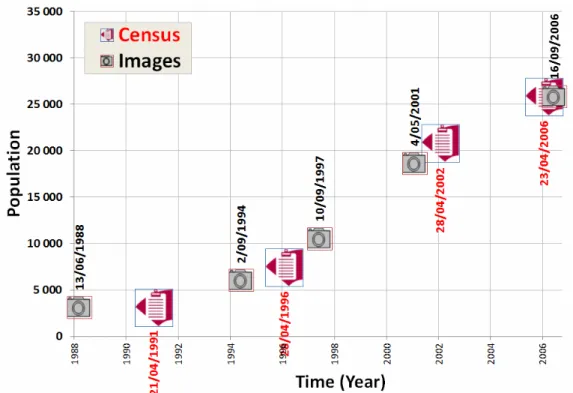
2.2.3. Population
Censuses are available per ward in April 1991, 1996, 2002 and 2006. Census data were pre-processed to get population at the acquisition instant of the images used to estimate sealed surface proportion. Linear interpolation was used to estimate the population in autumn 1994 and 1997 and summer 2001 and nearest neighbor was used for summer 1988 and 2006.
2.3. Model description and adjustment
Here is the regression model:
: Population of ward i, number of inhabitants from the census that has been normalized : Regression constant ‐ normalized see below number of inhabitants
: Cumulated weighted area in pixels of “other” land‐use class in ward i : Cumulated weighted area in pixels of “residential” land‐use class in ward i Cumulated weighted area in pixels of “commercial” land‐use class in ward i
: Regression coefficient of independent variable ‐ normalized density of inhabitants per pixe the “other” land‐use type
l in
: Regression coefficient o independent variable f ‐ normalized densi of inhabitants per pixel in the “residential” land‐use type
ty
: Regression coefficient o independent variable f ‐ normalized densi y of inhabitants per pixel in the “commercial” land‐use type
t
: Residual of ward i
The land use classes labeled “residential”, “commercial” and “other” are generalized MOLAND classes. The “residential” class aggregates all the residential classes of MOLAND. The “commercial” class corresponds to the MOLAND unique “Commercial areas” class. The class “other” aggregates two MOLAND classes, i.e. the “Industrial area” and “Public and private services”.
The cumulated weighted area of the 3 aggregated classes is computed using next equation:
: Number of pixels pertaining to aggregated class k k o, r or c in ward i : Sealed surface proportion image of land‐use class k in ward i
Different adjustment schemes can be adopted using the three dates with full data availability: - Remote sensing data of 1988 with census data of 1991 and MOLAND map of 1990
- Remote sensing data of 2001 with population linearly interpolated between census dates of 1996 and 2001 and MOLAND map of 2000
- Remote sensing data of 2006 with census data of 2006 and MOLAND map of 2006
In order to get a model that fits all the dates for forecasting purpose, the population of each ward is expressed in a normalized way dividing the ward population at a specified moment by the population of all the wards used in the adjustment at that date. It is then possible to make use of the observation equations of the 3 dates all together. The number of observation equations is therefore
three times the number of wards, if the same wards are used for all the dates depending on remote sensing coverage. We assume that a pixel of a specific land use with a definite imperviousness have a stable normalized density in time.
Two kinds of adjustments were afterward performed: (1) assuming a constant density component for all pixels pertaining to one of the 3 aggregated classes, i.e. the constant C is not null; (2) assuming no constant density component for those pixels, i.e. forcing the constant C to zero. The second assumption is physically more justified but induces careful interpretation of R².
2.4. Population disaggregation
The disaggregation was then applied separately on each date (1990, 2000, 2006) using the total population of that date or the mean total population of the 3 dates. This is to estimate the density in function of the land use in number of inhabitants per pixel rescaling the 3 regression coefficients, taking into account the global population of the date or the mean global population during the whole period. Of course this density is specific of a land use if it is 100% sealed. The spatial variation of the density within a land use class is then estimated from the sealed surface proportion map. This disaggregation procedure allows the population conservation for the whole area considered (where all data is available) all over the time period or at a specific date. A residual value can then be computed for each ward at each date using the model that is temporally representative of the whole past period.
The disaggregation strategy is explained below for two kinds of adjustments without or with forcing the constant C to zero.
In the first disaggregation approach, i.e. without forcing C to zero, we get from the model:
In this general equation, one can consider two values for N:
- N: Number of wards taken in consideration during the whole time period, i.e. 318 in 1990 + 317 in 2000 + 317 in 2006, if no outlier is removed. This disaggregation is defined as a “mean temporal disaggregation model”. The adjustment has been performed on the 3 dates.
Thus is null, if the 3 dates are combined in the disaggregation.
- N: Number of wards taken in consideration for one specific date, i.e. 318 in 1990, 317 in 2000 or 317 in 2006, if no outlier is removed. This disaggregation is defined as a “specific
date disaggregation model”. In this case, is not null.
In the disaggregation process, the term (N*C) is the contribution of a constant density on the population of a pixel, . It is assumed that the population related to this density is equally distributed in the whole weighted area covered by the 3 land use classes. The constant density term thus depends on the disaggregation model.
In the case of the “mean temporal disaggregation model” is formulated below: : number of p xels of land‐cover « other » i : number of pixels of land‐cover « residential » : number of pixels of land‐cover « commercial a : dates 1990, 2000 and 2006. »
In the case of a “specific date disaggregation model” is formulated above:
, and : same signification as above a : date 1990 or 2000 or 2006
In the general equation, , and are the estimated normalized density values on the land use. The disaggregation rule exploited to estimate the population corresponding to this term for a pixel of land use class k, depends on the land use class and on the sealed surface proportion of this pixel. Its value is computed using this equation:
“k” is the landuse i.e. “k” “o”, “r” or “c” : sealed surface proportion image
P : the total population that is conserved i.e. the mean total population of the 3 dates or the total population of a specific date
The disaggregation without forcing C to zero in the adjustment is computed by adding the constant density contribution to the variable population density depending on the land use, . In a pixel of land use class k, we thus get a population equal to .
In the second adjustment approach, i.e. forcing C to zero, the contribution of the constant density is null. We thus get a disaggregation value equal to .
In both disaggregation strategies, the process has been verified using a disaggregation –
re-aggregation procedure on the past dates before applying the model to forecast the spatial distribution of population. Of course the values of N, no, nr and nc were adapted to the outliers
3. Results
3.1. Model adjustment
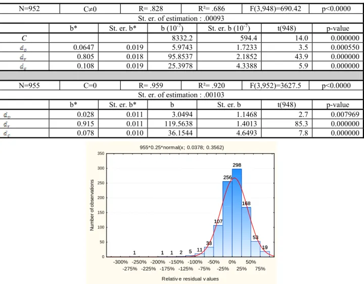
At the end of the first step, using the observations of the 3 dates and all the wards, a first set of values for C (if C is not forced to zero), , and . 23 and 21 outliers were removed depending on the adjustment strategy, respectively without and with zero-forcing for C. After the outliers removal, the final model was obtained. The results of both adjustment strategies are reported in Table 1. In both cases, R² value is highly significant, i.e. respectively 0.69 (F(3,948)=690.42, p<0.0000) and 0.92 (F(3,952)=3627.5, p<0.0000). The adjusted parameters are all conform (t-statistics). They are corresponding to the normalized density values for each land use class, if the sealed surface proportion is 100%. The rescaled and spatial-corrected density values are reported in Table 2. In both adjustments, the outliers were identified from the residuals histogram using a threshold of 2 . For their majority, the same wards are common to at least 2 of the 3 processed dates. These wards are mainly rural and the imperviousness is clearly overestimated because some agricultural plots with bare soil have been misclassified as urban.
Figure 2 shows the histogram of relative residual values for the whole time period. The histogram for specific dates not reported here, are very similar. This demonstrates the coherence of the model for the whole period.
Table 1. Parameters of the model adjusted on the 3 dates after the elimination of the outliers - models with C≠0 (above) and C forced to 0 (below). To interpret the values, note that the dependent variable in a normalized population.
N=952 C0 R= .828 R²= .686 F(3,948)=690.42 p<0.0000
St. er. of estimation : .00093
b* St. er. b* b (10-7) St. er. b (10-7) t(948) p-value
C 8332.2 594.4 14.0 0.000000 0.0647 0.019 5.9743 1.7233 3.5 0.000550 0.805 0.018 95.8537 2.1852 43.9 0.000000 0.108 0.019 25.3978 4.3388 5.9 0.000000 N=955 C=0 R= .959 R²= .920 F(3,952)=3627.5 p<0.0000 St. er. of estimation : .00103
b* St. er. b* b St. er. b t(948) p-value
0.028 0.011 3.0494 1.1468 2.7 0.007969 0.915 0.011 119.5638 1.4013 85.3 0.000000 0.078 0.010 36.1544 4.6493 7.8 0.000000 955*0.25*normal(x; 0.0378; 0.3562) 1 1 1 2 5 11 33 107 256 298 168 53 19 -300% -275% -250% -225% -200% -175% -150% -125% -100% -75% -50% -25% 0% 25% 50% 75% Relativ e residual v alues
0 50 100 150 200 250 300 350 N um b er of obs e rv at ions 1 1 1 2 5 11 33 107 256 298 168 53 19
Figure 2: Histogram of residual values expressed relatively to the true value [(true-estimated) divided by the true value] for the 3 dates – model forcing C to zero after the elimination of 21 outliers.
3.2. Validation of the disaggregation process at 30 m resolution
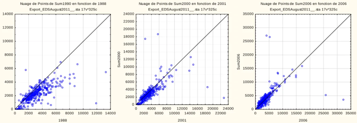
The disaggregation process was then validated using a disaggregation - reaggregation procedure. The reaggregation was performed in each ward allowing the creation of validation plots (Figure 3) to compare the reaggregated population with the actual population using a mean global population over time or a date-specific global population as population rescaling factor. The outliers are obvious on the plots. Both population rescaling methods have the same accuracy and precision. The population for 1988 is clearly under-estimated by the model. The precision is also lower for this date. The bias is almost inexistent for the two other dates but the result for 2006 is clearly more precise. This is probably due to a better estimation of sealed surface proportion done from a SPOT image with a higher resolution.
Nuage de Points de Sum1990 en fonction de 1988 Export_EDSAugust2011__.sta 17v*325c 0 2000 4000 6000 8000 10000 12000 14000 1988 0 2000 4000 6000 8000 10000 12000 14000 S um 199 0
Nuage de Points de Sum2000 en fonction de 2001 Export_EDSAugust2011__.sta 17v*325c 0 2000 4000 6000 8000 10000 12000 14000 16000 18000 20000 22000 24000 2001 0 2000 4000 6000 8000 10000 12000 14000 16000 18000 20000 22000 24000 Su m 2 0 0 0
Nuage de Points de Sum2006 en fonction de 2006 Export_EDSAugust2011__.sta 17v*325c 0 5000 10000 15000 20000 25000 30000 35000 2006 0 5000 10000 15000 20000 25000 30000 35000 S um 200 6
Figure 3: Validation plots comparing the population per ward after the disaggregation – reaggregation procedure (Y) with the true population (X) for 1988 (left), 2001 (center) and 2006 (right); a global population specific to each date was
used to rescale the population from normalized output of the model – model forcing C to zero. 3.3. Testing the disaggregation - reaggregation at 200 m resolution
Because the land use forecasting has been performed at a resolution of 200 m, our model was tested at this coarser resolution for the year 2006. The scope of this test is the verification of the resolution effect on the result of the disaggregation. The validation plot (Figure 4) demonstrates that the application of the model at 200 m resolution is thus fully consistent with the former tests at 30 m resolution. One may thus make use of it to forecast the spatial distribution of the population from predicted land use and imperviousness maps at 200 m resolution.
Nuage de Points de TIM200m en f onction de 2006 Export_200m sur Export_200m.stw 17v*325c
0 5000 10000 15000 20000 25000 30000 35000 2006 0 5000 10000 15000 20000 25000 30000 35000 TI M 2 0 0 m
Figure 4: Validation plot of the disaggregation model test at 200 m resolution for 2006 (Y = model output - X = true population) - model forcing C to zero and date-specific global population.
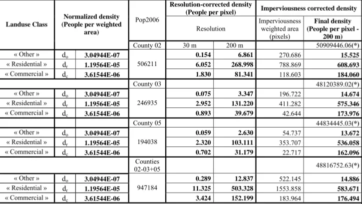
Table 2 shows the results of other tests performed conserving the population in each of the 3 counties processed or globally on those counties. This table provides the density values for each land use type. The computation of these density values are corrected accordingly to the pixel resolution (“Resolution-corrected density”) and to the weighted area processed, because all the wards are not totally covered by the used images in the sealed surface proportion estimation or missing value pixels exist because of clouds (“Imperviousness corrected density”). Figure 5 shows the corresponding disaggregated population map and its spatial validation.
Table 2. Population density per land use class.
Resolution-corrected density
(People per pixel) Imperviousness corrected density
Pop2006 Resolution Imperviousness weighted area (pixels) Final density (People per pixel -
200 m) Landuse Class
Normalized density (People per weighted
area) County 02 30 m 200 m 50909446.06(*) « Other » do 3.04944E-07 0.154 6.861 270.686 15.525 « Residential » dr 1.19564E-05 6.052 268.998 788.869 608.693 « Commercial » dc 3.61544E-06 506211 1.830 81.341 118.603 184.060 County 03 48120389.02(*) « Other » do 3.04944E-07 0.075 3.347 196.722 14.674 « Residential » dr 1.19564E-05 2.952 131.220 411.282 575.346 « Commercial » dc 3.61544E-06 246935 0.893 39.679 42.644 173.976 County 05 44834445.03(*) « Other » do 3.04944E-07 0.059 2.630 54.737 13.672 « Residential » dr 1.19564E-05 2.320 103.111 353.707 536.058 « Commercial » dc 3.61544E-06 194038 0.702 31.179 22.717 162.096 Counties 02-03+05 48816752.63(*) « Other » do 3.04944E-07 0.289 12.837 522.145 14.886 « Residential » dr 1.19564E-05 11.325 503.328 1553.858 583.671 « Commercial » dc 3.61544E-06 947184 3.424 152.199 183.964 176.494
(*) density correction factor taking into account the resolution and the total imperviousness of each landuse class
Underestimation (positive residual values) of population inside of the city is due to the underestimation of density associated to the 3 land use classes and to the saturation of the imperviousness at the maximum level. Moreover, a lot of buildings are used for accommodation but are classified as “commercial” or “other” and characterised by much lower densities than the
“residential” class. The blue belt mainly observed at the southern periphery of Dublin corresponds to overestimated wards’ population (negative residual values). The modelled densities
are probably too high with regard to the morphology of the residential zones in this urban fringe. Furthermore, the excessive spatial generalisation of the MOLAND land use map produces rough partitioning of the three classes with overestimation of the area where people live. Possibly this is also influenced by the disproportionate effect of imperviousness in this area overestimation. Finally, population underestimation (reddish southern belt) in large rural wards far away of the city is possibly due to the underestimation of the build-up area eventually linked to too lower imperviousness. The very smaller number of inhabitants can also produce there high positive residual values because this is expressed relatively to the actual population. Of course the largest positive or negative residual values correspond to the wards that were identified as outliers where the model has been applied anyway.
Figure 5: Left: Disaggregation result at 200 m resolution for 2006 - model forcing C to zero and population rescaling
using the global population specific to the date 2006.
Right: Spatial distribution of residual values expressed relatively to the true value, i.e. [(true - estimated) divided by the true value]. The result shown is obtained with a density correction applied separately on the 3 counties and the output of
the sealed surface estimate (see table 2).
4. Conclusion
The use of sealed surface obtained from time series of past medium resolution remotely sensed images in combination with land use maps is a helpful improvement of the traditional regression based dasymetric model using remote sensing data. As stated by the validation process, the adjustment and the density estimation strategies have been adequately designed to spatial extrapolation and forecasting.
Of course the forecasting relies on the outputs of models simulating urban dynamics that are available in the MOLAND project [26]. Furthermore, the forecasting also relies on the future evolution of the surface imperviousness, which is the subject of ongoing research.
Our model can be fed by these simulated data to predict the spatial distribution of population assuming that future association between density and land use through surface imperviousness shall remain stable. Obviously this mainly depends on the functional and morphological evolution of the cities in relation to urban policy, macro-economical circumstances and people behaviour with regards to their living and working environment.
Acknowledgement
This publication is a result of the MAMUD project (SR/00/105) financed by the Belgian Science Policy Office (BELSPO).
References
[1] Noin, D., 1979. Géographie de la population. Masson, Paris, 320 p.
[2] Lavalle, C., Demicheli, L., Turchini, M., Casals-Carrasco, P. and Niederhuber, M., 2001. Monitoring megacities; the MUR- BANDY/MOLAND approach. Dev. Prac. 11, pp. 350–357.
[3] White, R., Engelen, C., Uljee, I., Lavalle, C. and Erlich, D., 1999. Developing an urban land use simulator for
European cities. In: Proceedings of the 5th EC-GIS Workshop, Stresa, Italy.
[4] Holt, J. B. and Lu, H., 2011. Dassymetry mapping for population and socio-demographic data distribution.
in Urban remote sensing. Monitoring, synthesis, and modeling of the urban environment (Xiaojun Yang ed.),
Wiley-Blackwell, pp. 195-210.
[6] Eicher, C. L., and Brewer, C. A., 2001. Dasymetric mapping and areal interpolation: implements and evaluation.
Cartography and Geographic Information Science, Vol. 28, N° 2, pp. 125-138.
[7] Hawley, 2005. A comparative analysis of areal interpolation methods. Master of Arts Thesis, Ohio State
University, Geography, 88 p.
[8] Mennis, J., and Hultgren, T., 2006. Intelligent dasymetric mapping and its application to areal interpolation.
Cartography and Geographic Information Science, Vol. 33, N° 3, pp. 179-194.
[9] Openshaw, S., 1984. The Modifiable Areal Unit Problem. CATMOG 38. Geo Books. Norwich. 41 p.
[10] Fotheringham, A. S., Brunsdon, C., & Charlton, M. E., 2002. Geographically Weighted Regression: The Analysis
of Spatially Varying Relationships. Wiley, Chichester, 273 p.
[11] Tobler, W., 1969. Satellite confirmation of settlement size coefficients. Area, Vol. 1, pp. 30-34.
[12] Cornet, Y., Binard, M., Laplanche, F., and Lambotte, J. M., submitted 2011. 2D and 3D data in mobility and
planning application. Bulletin de la Société Géographique de Liège.
[13] Ledant, M., 2009. Evaluation du potentiel de la cartographie densimétrique appliquée à des données de très grande
échelle spatiale 2D et 3D. Le cas de la région liégeoise. Master thesis in geographical sciences, University of Liège.
[14] Isaka, J., and Hegedus, E., 1982. Population estimation from Landsat imagery. Remote Sensing of Environment,
Vol. 12, pp. 259–272.
[15] Lo, C. P., 1995. Automated population and dwelling unit estimation from high resolution satellite images: a GIS
approach. International Journal of Remote Sensing, Vol. 16, pp. 17–34.
[16] Harvey, J.T., 2002. Estimation census district population from satellite imagery: some approaches and limitations.
International Journal of Remote Sensing, Vol. 23, pp. 2071-2095.
[17] Peplies, R. W., 1974. Regional analysis and remote sensing: a methodological approach. In: Estes, J. E. (eds.),
Remote sensing: techniques for environmental analysis, pp. 277-291.
[18] Haack, B. N., Guptill, S. C., Holz, R. K., Jampoler, S. M., Jensen, J. R. and Welch, R. A., 1997. Urban analysis and
planning. In: Philipson et al. (Eds.), Manual of photographic interpretation, 2. Ed, American Society for Photogrammetry & Remote Sensing, Bethesda, pp. 517-554.
[19] Herold, M, Liu, X. and Clarke, K. C., 2003. Spatial metrics and image texture for mapping urban land-use.
Photogrammetric Engineering and Remote Sensing, Vol. 69, N° 9, pp. 991-1001.
[20] Liu, X., Clarke, K.-C., and Herold, M., 2006. Population density and image texture: a comparison study.
Photogrammetric Engineering and Remote Sensing, Vol. 72, N° 2, pp. 187-196.
[21] Liu, X. and Herold, M., 2007. Estimating population distributions in urban areas. In: Weng, Q. & D. Quattrochi
(Eds.), Urban remote sensing, Taylor & Francis, pp. 269-290.
[22] Langford, M., Maguire, D. J., and Unwin, D. J. 1991. The areal interpolation problem: estimating population using remote sensing in a GIS Framework. In: Masser, I. & M. Blakemore (Eds.), Handling geographical information:
methodology and potential applications, Wiley, New York, pp. 55-77.
[23] Donnay, J. P., and Unwin, D., 2001. Modelling geographical distributions in urban areas. In: Donnay, Jean-Paul,
Barnsley, M., and Longley, P. (Eds.), Remote Sensing and Urban Analysis, Taylor & Francis, London, pp. 205-224.
[24] Van de Voorde T., Demarchi L., and Canters F., 2009a. Multi-temporal spectral unmixing to characterise urban
change in the Greater Dublin area, 28th EARSeL Symposium –Remote Sensing for a Changing Europe, 2-7 June 2008, Istanbul, Turkey, IOS Press, pp 276-283.
[25] Van de Voorde T., De Roeck T. and Canters, F., 2009b. A comparison of two spectral mixture modelling
approaches for impervious surface mapping in urban areas, International Journal of Remote Sensing, vol. 30 (18), pp. 4785 – 4806.
[26] van der Kwast J., Van de Voorde T., Binard M., Engelen G., Cornet Y., Uljee I., Lavalle C., Canters F., Poelmans
P., Shahumyan H., Williams B. and Convery S. (in review). Using spatial metrics derived from remote sensing for the calibration of land-use change models. Landscape and Urban Planning.