HAL Id: hal-01314470
https://hal.archives-ouvertes.fr/hal-01314470
Submitted on 11 May 2016
HAL is a multi-disciplinary open access
archive for the deposit and dissemination of
sci-entific research documents, whether they are
pub-lished or not. The documents may come from
teaching and research institutions in France or
abroad, or from public or private research centers.
L’archive ouverte pluridisciplinaire HAL, est
destinée au dépôt et à la diffusion de documents
scientifiques de niveau recherche, publiés ou non,
émanant des établissements d’enseignement et de
recherche français ou étrangers, des laboratoires
publics ou privés.
Abducing Biological Regulatory Networks from Process
Hitting models
Maxime Folschette, Loïc Paulevé, Katsumi Inoue, Morgan Magnin, Olivier
Roux
To cite this version:
Maxime Folschette, Loïc Paulevé, Katsumi Inoue, Morgan Magnin, Olivier Roux. Abducing Biological
Regulatory Networks from Process Hitting models. ECML-PKDD 2012 Workshop on Learning and
Discovery in Symbolic Systems Biology, Sep 2012, Bristol, United Kingdom. �hal-01314470�
Abducing Biological Regulatory Networks from
Process Hitting models
Maxime Folschette1,2, Loïc Paulevé3, Katsumi Inoue2, Morgan Magnin1,
Olivier Roux1
1 LUNAM Université, École Centrale de Nantes, IRCCyN UMR CNRS 6597
(Institut de Recherche en Communications et Cybernétique de Nantes) 1 rue de la Noë – B.P. 92101 – 44321 Nantes Cedex 3, France.
2
National Institute of Informatics,
2-1-2, Hitotsubashi, Chiyoda-ku, Tokyo 101-8430, Japan.
3
LIX, École Polytechnique, 91128 Palaiseau Cedex, France.
Abstract. The Process Hitting (PH) is a recently introduced framework to model concurrent processes. It is notably suitable to model Biological Regulatory Networks (BRNs) with partial knowledge of cooperations by defining the most permissive dynamics. On the other hand, the qualita-tive modeling of BRNs has been widely addressed using René Thomas’ formalism. Given a PH model of a BRN, we first tackle the inference of the underlying Interaction Graph between components. Then the in-ference of corresponding Thomas’ models is provided by inferring some parameters and abducing the compatible parametrizations.
1
Introduction
As regulatory phenomena play a crucial role in biological systems, they need to be studied accurately. Biological Regulatory Networks (BRNs) consist in sets of either positive or negative mutual effects between the components. Besides continuous models of physicists, often designed through systems of ordinary dif-ferential equations, a discrete modeling approach was initiated by René Thomas in 1973 [1] allowing the representation of the different levels of a component, such as concentration or expression levels, as integer values. Nevertheless, these dynamics can be precisely established only with regard to some kind of “focal points”, related to as Thomas’ parameters, indicating the evolutionary tendency of each component.
Thomas’ modeling has motivated numerous works around the link between the influences and the possible dynamics (e.g., [2]), model reduction (e.g., [3]), or the incorporation of time (e.g., [4,5]) to name but a few. Other approaches related to our work, which rely on on temporal logic [6] and constraint program-ming [7,8], aim at determining models consistent with partial data on the regula-tory structure and dynamics. While the formal checking of dynamical properties is often limited to small networks because of the state graph explosion, the main
drawback of this framework is the difficulty to specify Thomas’ parameters, es-pecially for large networks. In our approach, we intend to focus on the Thomas’ parameters inference.
In order to address the formal checking of dynamical properties within very large BRNs, we recently introduced in [9] a new formalism, named the “Pro-cess Hitting” (PH), to model concurrent systems having components with a few qualitative levels. A PH describes, in an atomic manner, the possible evolutions of a “process” (representing one component at one level) triggered by the hit of at most one other “process” in the system. This particular structure makes the formal analysis of BRNs with hundreds of components tractable [10]. A PH model can be built based on information found in the literature about the local influences between components. It is then suitable, according to the precision of this information, to model BRNs with different levels of abstraction by capturing the most general dynamics.
In this work4, we show that starting from one PH model, it is possible to find the underlying interactions. We perform an exhaustive search for the pos-sible interactions on one component from all the others, consistently with the knowledge of the dynamics expressed in PH. The second phase of our work con-cerns the Thomas’ parameters inference. It consists in abducing the (possibly large) nesting set of parameters which, together with other given conditions, suf-ficiently derives satisfaction of the known cooperating constraints. The resulting dynamics are ensured to respect the PH dynamics, i.e. no spurious transitions are made possible.
The first benefit of our approach is that it makes possible the construction refining of BRNs with a partial and progressively brought knowledge in PH, while being able to export such models in the Thomas’ framework. Our second contribution is to enhance the knowledge of the formal links between both mod-elings. As BRNs are not limited to Boolean values, the whole method can be applied to multi-valued models; furthermore, the method can be applied to large BRNs (up to 40 components).
Outline. Sect. 2 recalls the PH and Thomas frameworks; Sect. 3 defines the IG inference from PH; Sect. 4 details the enumeration of Thomas parametrizations compatible with a PH; Sect. 5 gives some information about the implementation of the method.
2
Frameworks
2.1 The Process Hitting framework
A Process Hitting (PH) (Def. 1) gathers a finite number of concurrent processes grouped into a finite set of sorts. A sort stands for a component of the system while a process, which belongs to a unique sort, stands for one of its expression levels. A process is thus noted aiwhere a is the sort and i is the process identifier
4
within the sort a. At any time, exactly one process of each sort is present; a state of the PH thus corresponds to such a set of processes.
The concurrent interactions between processes are defined by a set of actions. Actions describe the replacement of a process by another of the same sort con-ditioned by the presence of at most one other process in the current state. An action is denoted by ai→ bj bk, which is read as “ai hits bj to make it bounce
to bk”, where ai, bj, bk are processes of sorts a and b, called respectively hitter,
target and bounce of the action.
Definition 1 (Process Hitting). A Process Hitting is a triple (Σ, L, H): – Σ = {a, b, . . . } is the finite set of sorts;
– L = Q
a∈ΣLa is the set of states with La = {a0, . . . , ala} the finite set of
processes of sort a ∈ Σ and la a positive integer, with a 6= b ⇒ ∀(ai, bj) ∈
La× Lb, ai6= bj;
– H = {ai→ bj bk, · · · | (a, b) ∈ Σ2∧ (ai, bj, bk) ∈ La× Lb× Lb
∧bj 6= bk∧ a = b ⇒ ai= bj} is the finite set of actions.
Given a state s ∈ L, the process of sort a ∈ Σ present in s is denoted by s[a]. An action h = ai→ bj bk∈ H is playable in s ∈ L if and only if s[a] = ai and
s[b] = bj. In such a case, (s · h) stands for the state resulting from the play of
the action h in s, with (s · h)[b] = bk and ∀c ∈ Σ, c 6= b, (s · h)[c] = s[c].
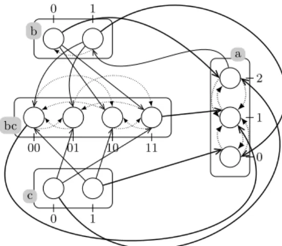
Modeling cooperation. As described in [9], the cooperation between processes to make another bounce can be expressed in PH by building a cooperative sort. Fig. 1 shows an example of a cooperative sort bc between sorts b and c, defined with 4 processes (one for each sub-state of the presence of processes b1 and
c1). For the sake of clarity, processes of bc are indexed using the sub-state they
represent. Hence, bc01 represents the sub-state hb0, c1i, and so on. Each process
of sort b and c hit bc to make it bounce to the process reflecting the status of the sorts b and c (e.g., b1 → bc00 bc10 and b1 → bc01 bc11). Then, to represent
the cooperation between processes b1and c1, the process bc11hits a1to make it
bounce to a2 instead of independent hits from b1 and c1. The same cooperative
sort is used to make b0 and c0 cooperate to hit a1 and make it bounce to a0.
We note that cooperative sorts are standard PH sorts and do not involve any special treatment regarding the semantics of related actions. However, it is worth noticing they introduce a temporal shift in their application. This allows the existence of interleaving of actions leading to a cooperative sort represent-ing a past sub-state of the presence of the cooperative processes. The resultrepresent-ing behavior is then an over-approximation of the realization of an instantaneous cooperation.
Example. Fig. 1 represents a PH (Σ, L, H) with especially: Σ = {a, b, c, bc}, La = {a0, a1, a2}, Lb = {b0, b1}, Lc = {c0, c1} and Lbc= {bc00, bc01, bc10, bc11}.
This example models a BRN where the component a has three qualitative levels, components b and c are Boolean and bc is a cooperative sort. In this BRN, a inhibits b at level 2 while b and c activate a with independent actions (e.g.
b0→ a2 a1) or through the cooperative sort bc (e.g. bc11 → a1 a2). Indeed,
the reachability of a2 and a0 is conditioned by a cooperation of b and c, as
explained above. b 0 1 c 0 1 a 0 1 2 bc 00 01 10 11
Fig. 1. A PH example with four sorts: three components (a, b and c) and a cooperative sort (bc). Actions targeting processes of a are in thick lines.
2.2 Thomas’ modeling
Thomas’ formalism, here inspired by [12,13], lies on two complementary descrip-tions of the system. First, the Interaction Graph (IG) models the structure of the system by defining the components’ mutual influences. Its nodes represent components, while its edges labeled with a threshold stand for either positive or negative interactions (Def. 2); la denotes the maximum level of a component a.
Definition 2 (Interaction Graph). An Interaction Graph (IG) is a triple (Γ, E+, E−) where Γ is a finite number of components, and E+ (resp. E−)
⊂ {a−→ b | a, b ∈ Γ ∧ t ∈ [1; lt a]} is the set of positive (resp. negative) regulations
between two nodes, labeled with a threshold.
A regulation from a to b is uniquely referenced: if a−→ b ∈ Et + (resp. E−),
then @a t
0
−→ b ∈ E+ (resp. E−), t0 6= t and @a t0
−→ b ∈ E− (resp. E+), t0 ∈ N.
For an interaction of the IG to take place, the expression level of its head com-ponent has to be higher than its threshold; otherwise, the opposite influence is expressed. For any component a ∈ Γ , Γ−1(a) = {b ∈ Γ | ∃b−→ a ∈ Et +∪ E−}
is the set of its regulators. A state s of an IG (Γ, E+, E−) is an element in
Q
a∈Γ[0; la] and s[a] refers to the level of component a in s.
Then, the specificity of Thomas’ approach lies in the use of discrete param-eters to represent focal level intervals (Def. 3). While the use of intervals as
a
b
c
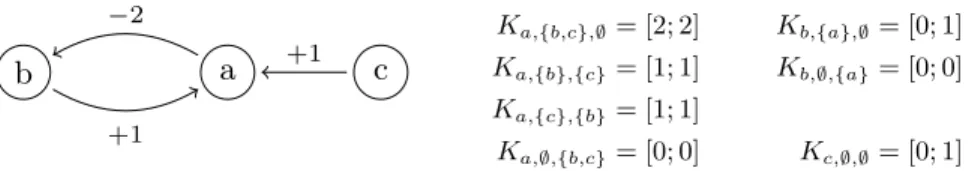
+1 +1 −2 K a,{b,c},∅= [2; 2] Kb,{a},∅= [0; 1] Ka,{b},{c}= [1; 1] Kb,∅,{a}= [0; 0] Ka,{c},{b}= [1; 1] Ka,∅,{b,c}= [0; 0] Kc,∅,∅= [0; 1]Fig. 2. (left) IG example. Regulations are represented by the edges labeled with their sign and threshold. For instance, the edge from b to a is labeled +1, which stands for: b−→ a ∈ E1 +. (right) Example parametrization of the left IG.
parameters does not add expressivity in Boolean networks, it allows to specify a larger range of dynamics in the general case (w.r.t. a fixed IG).
Definition 3 (Discrete parameter Kx,A,B and Parametrization K). Let
x ∈ Γ be a given component and A (resp. B) ⊂ Γ−1(x) a set of its activators (resp. inhibitors), such that A ∪ B = Γ−1(x) and A ∩ B = ∅. The discrete pa-rameter Kx,A,B = [i; j] is a non-empty interval so that 0 ≤ i ≤ j ≤ lx. With
regard to the dynamics, x will tend towards Kx,A,B in the states where its
acti-vators (resp. inhibitors) are the regulators in set A (resp. B). The complete map K = (Kx,A,B)x,A,B of discrete parameters for an IG is called a parametrization
of this IG.
At last, dynamics are defined in BRN in an unitary and asynchronous way: from a given state s, a transition to another state s0 is possible provided that only one component a will evolve of exactly one level towards Ka,A,B, where A
(resp. B) is the set of activators (resp. inhibitors) of a in s.
Example. Fig. 2(left) represents an Interaction Graph (Γ, E+, E−) with Γ =
{a, b, c}, E+ = {b 1 −→ a, c −→ a} and E1 − = {a 2 − → b}; hence Γ−1(a) = {b, c}.
Fig. 2(right) gives a possible parametrization on this IG. In this BRN, the following transitions are possible: ha0, b1, c1i → ha1, b1, c1i → ha2, b1, c1i →
ha2, b0, c1i → ha1, b0, c1i, where ai is the component a at level i.
3
Interaction Graph Inference
In order to infer a complete BRN, one has to find the Interaction Graph (IG) first, as some constraints on the parametrization rely on it. Inferring the IG is an abstraction step which consists, from atomistic actions of a PH, in determining the global influence of every component on each of its successors. We consider hereafter a global PH (Σ, L, H) on which the IG inference is to be performed.
We denote context a set ς of processes that are potentially active. Many of the inferences defined in the rest of this paper rely on the knowledge of focal processes focals(a, Sa, ς) amongst a subset Sa ⊂ La of the processes of a sort a,
context ς and whose targets are in Sa; we call G the digraph whose edges are
{(aj; ak) | bi→ aj ak ∈ H} and nodes are Sa∪ {aj, ak | bi → aj ak∈ H}.
– If G is acyclic, we define focals(a, Sa, ς) as the set of nodes of G with no
outgoing edge, i.e. the set of processes of a that are the bounce of an action in H but that are not the target of any action in H. Thus, if focals(a, Sa, ς)
is not empty, we expect, starting from a process in Sa and under some
conditions on ς, to always reach one focal process in a bounded number of actions.
– If G contains a cycle, then focals(a, Sa, ς) = ∅ as there exists a sequence of
actions in H that can be played successively in a loop. Example. In the PH of Fig. 1, we obtain:
focals(a, La, {bc00}) = {a0} focals(a, La, {bc11}) = {a2}
focals(a, La, {bc10}) = {a1} focals(a, La, {bc01}) = {a1}
3.1 Well-formed Process Hitting for Interaction Graph Inference
The inference of an IG from a PH assumes that the PH defines two types of sorts: the sorts corresponding to BRN components, that will appear in the IG, and the cooperative sorts. The identification of sorts modeling components relies on the observation that their processes represent (ordered) qualitative levels; hence, to respect BRNs dynamics, an action on such a sort cannot make it bounce to a process at a distance more than one. Any sort that does not act as a component should then be treated as a cooperative sort, whose role is to compute the current state of set of cooperating processes, as explained in Subsect. 2.1. Thus, for each sub-state of its predecessors, a cooperative sort should converge to a unique focal process. In addition of having either component sorts or cooperative sorts, we also require that there is no cycle between cooperative sorts, and that sorts being never hit (i.e. serving as an invariant environment) are components.
Example. In the PH of Fig. 1, a, b and c are valid components as they repsect the above conditions. Furthermore, bc is a valid cooperative sort as:
∀i, j ∈ {0, 1}, focals(bc, Lbc, {bi, cj}) = {bcij}
3.2 Interaction Inference
Inferring the underlying IG of a PH consists in finding the influence of each regulator of every component, in order to determine the sets E+ and E−. We
aim at inferring that b activates (inhibits) a if there exists a configuration where increasing the level of b makes possible the increase (decrease) of the level of a. Inferring a global influence requires to focus on local influences first. We rely on the search of local influence switches of b on a that point out local changes in this influence (activations or inhibitions) between levels biand bi+1. It is also
the evolution of a also depends on them. This method compares the set of focal processes of a in a context containing bi and some cooperating processes, and
in the same context containing bi+1; a positive (resp. negative) local influence
switch is found if the former is higher (resp. lower) than the latter, regarding an appropriate comparison relation on sets of processes. If both sets are identical, no local influence switch is inferred as the influence of b on a is the same for both bi and bi+1 in this context.
Once all local influence switches of b on a have been found (for all couples of bi and bi+1, and all contexts of other components cooperating with b to hit a),
we are able to infer a positive (resp. negative) edge if there exist only positive (resp. negative) local influence switches of b on a. The threshold of such an edge is the minimum threshold for which an influence switch has been found. We infer an unsigned edge (with non threshold) if two influence switches of different types are found.
Example. In the PH of Fig. 1, we have:
focals(b, Lb, {a0}) = {b0, b1} focals(b, Lb, {a2}) = {b0}
focals(b, Lb, {a1}) = {b0, b1}
Therefore, we infer a negative influence switch of a on b between levels a1 and
a2, but not between a0 and a1, because:
focals(b, Lb, {a0}) = focals(b, Lb, {a1})
focals(b, Lb, {a1}) focals(b, Lb, {a2})
We thus deduce that: a−→ b ∈ E2 −.
Indeed, the IG inference from the PH of Fig. 1 gives E+ = {b 1 − → a, c−→ a}1 and E−= {a 2 −
→ b}, corresponding to the IG of Fig. 2.
4
Parametrization inference
Given the IG inferred from a PH as presented in the previous section, one can find the discrete parameters that model the behavior of the studied PH using the method presented in the following. As some parameters may remain undeter-mined, another step allows to enumerate all parametrizations compatible with the inferred parameters.
4.1 Independent parameters inference
This subsection presents some results related to the inference of independent discrete parameters from a given PH, equivalent to those presented in [9]. We suppose in the following that the considered PH is well-formed for parameters inference: its inferred IG does not contain any unsigned edge, and in each sort, all
processes activating (resp. inhibiting) another component share the same behav-ior. Let Ka,A,B be the parameter we want to infer for a given component a ∈ Γ
and A ⊂ Γ−1(a) (resp. B ⊂ Γ−1(a)) a set of its activators (resp. inhibitors). This inference, as for the IG inference, relies on the search of focal processes of the component for the given configuration of its regulators.
For each sort b ∈ Γ−1(a), we define a context that contains all processes of b activating (resp. inhibiting) a if b ∈ A (resp. B). From all contexts of all predecessors of a, we create a global context that represents the configuration A, B (including the cooperative sorts involved). The parameter Ka,A,B specifies
towards which values a eventually evolves as long as this context holds, which is precisely given by the set of focal processes.
Example. In the PH of Fig. 1, we have in particular:
focals(b, Lb, {a0, a1}) = {b0, b1}, which gives: Kb,{a},∅= [0; 1],
focals(a, La, {b1, c1, bc11}) = {a2}, which gives: Ka,{b,c},∅= [2; 2], and
focals(a, La, {b1, c0, bc10}) = {a1}, which gives: Ka,{b},{c}= [1; 1].
This method sometimes faces cases with opposite effects on a component, leading to either an indeterministic evolution or to oscillations. Such an indeter-minism is not possible in a BRN, and the inference of the targeted parameter is impossible. In order to avoid such inconclusive cases, one has to ensure that no such behavior is allowed by either removing undesired actions or using cooper-ative sorts to prevent opposite influences between regulators.
4.2 Abductive reasoning to find admissible parametrizations
In the following, we try to constrain all parameters that are left undetermined with the method presented in the previous subsection. We consider that a pa-rameter is valid if any transition it involves in the resulting BRN is allowed by the studied PH by actions that represent this behavior. We also add some biolog-ical constraints on the whole parametrizations, given in [13]. These constraints lead to a family of admissible parametrizations which we can enumerate and are ensured to observe a coherent behavior that is included in the original PH.
This approach can be considered as abductive reasoning as some information is added by the enumeration. If we denote:
– M the fact that the behavior of the resulting BRN observes the dynamics of the PH,
– B the fact (which is granted) that the IG and the series of necessary param-eters inferred from the PH are parts of the resulting BRN,
– HK the hypothesis that K is an admissible complete parametrization,
then the parametrizations K that answer our expectations are the ones so that: – HK is compatible with B, that is, all parameters of K are compatible with
– B ∧ HK |= M , that is, the inferred IG together with K represent a BRN
observing the behavior included into the dynamics of the original PH. Answer Set Programming (ASP) [14] turns out to be effective for the enu-merative searches developed in this paper, as it efficiently tackles the inherent complexity of the models we use, thus allowing an efficient execution of the formal tools developed. Furthermore, ASP finds a particularly interesting appli-cation in the research of admissible parametrizations regarding the properties presented above, as this enumeration can be naturally formulated with the use of aggregates, and constraints allow to remove all non-admissible models.
5
Implementation
The inference method described in this paper has been implemented as a tool named ph2thomas, as part of Pint5, which gathers PH related tools. Our im-plementation mainly consists in ASP programs that are solved using Clingo6.
In the previous sections and in the appendix, we illustrate our results on toy examples considered as small networks. But our approach can also success-fully handle large PH models of BRNs found in the literature such as an ERBB receptor-regulated G1/S transition model from [15] which contains 20 compo-nents, and a T-cells receptor model from [16] which contains 40 components7.
For each model, IG and parameters inferences are performed together in less than a second on a standard desktop computer.
6
Conclusion
This work establishes the abstraction relationship between PH, which is more abstract and allows incomplete knowledge on cooperations, and Thomas’ ap-proach for qualitative BRN modeling. This motivates the concretization of PH models into a set of compatible Thomas’ models using abduction in order to benefit of the complementary advantages of these two formal frameworks and extract some global information about the influences between components.
As an extension of the presented work, we plan to explore new semantics of BRNs to be able to tackle influences currently represented by unsigned edges. Ack. This work was partially supported by the Fondation Centrale Initiatives.
References
1. Thomas, R.: Boolean formalization of genetic control circuits. Journal of Theoret-ical Biology 42(3) (1973) 563 – 585
5 Available at http://process.hitting.free.fr 6
Available at http://potassco.sourceforge.net
7
2. Richard, A., Comet, J.P.: Necessary conditions for multistationarity in discrete dynamical systems. Discrete Applied Mathematics 155(18) (2007) 2403 – 2413 3. Naldi, A., Remy, E., Thieffry, D., Chaouiya, C.: A reduction of logical regulatory
graphs preserving essential dynamical properties. In: Computational Methods in Systems Biology. Volume 5688 of LNCS. Springer (2009) 266–280
4. Siebert, H., Bockmayr, A.: Incorporating time delays into the logical analysis of gene regulatory networks. In: Computational Methods in Systems Biology. Volume 4210 of LNCS. Springer (2006) 169–183
5. Ahmad, J., Roux, O., Bernot, G., Comet, J.P., Richard, A.: Analysing formal models of genetic regulatory networks with delays. International Journal of Bioin-formatics Research and Applications (IJBRA) 4(2) (2008)
6. Khalis, Z., Comet, J.P., Richard, A., Bernot, G.: The SMBioNet method for discov-ering models of gene regulatory networks. Genes, Genomes and Genomics 3(spe-cial issue 1) (2009) 15–22
7. Corblin, F., Fanchon, E., Trilling, L.: Applications of a formal approach to decipher discrete genetic networks. BMC Bioinformatics 11(1) (2010) 385
8. Corblin, F., Fanchon, E., Trilling, L., Chaouiya, C., Thieffry, D.: Automatic infer-ence of regulatory and dynamical properties from incomplete gene interaction and expression data. In: IPCAT. Volume 7223 of LNCS., Springer (2012) 25–30 9. Paulevé, L., Magnin, M., Roux, O.: Refining dynamics of gene regulatory networks
in a stochastic π-calculus framework. In: Transactions on Computational Systems Biology XIII. Springer (2011) 171–191
10. Paulevé, L., Magnin, M., Roux, O.: Static analysis of biological regulatory networks dynamics using abstract interpretation. Mathematical Structures in Computer Science in press (2012) Preprint: http://loicpauleve.name/mscs.pdf.
11. Folschette, M., Paulevé, L., Inoue, K., Magnin, M., Roux, O.: Concretizing the process hitting into biological regulatory networks. In: Computational Methods in Systems Biology, Springer (2012)
12. Richard, A., Comet, J.P., Bernot, G.: Formal Methods for Modeling Biological Regulatory Networks. In: Modern Formal Methods and App. (2006) 83–122 13. Bernot, G., Cassez, F., Comet, J.P., Delaplace, F., Müller, C., Roux, O.:
Seman-tics of biological regulatory networks. Electronic Notes in Theoretical Computer Science 180(3) (2007) 3 – 14
14. Baral, C.: Knowledge Representation, Reasoning and Declarative Problem Solving. Cambridge University Press (2003)
15. Sahin, O., Frohlich, H., Lobke, C., Korf, U., Burmester, S., Majety, M., Mattern, J., Schupp, I., Chaouiya, C., Thieffry, D., Poustka, A., Wiemann, S., Beissbarth, T., Arlt, D.: Modeling ERBB receptor-regulated G1/S transition to find novel targets for de novo trastuzumab resistance. BMC Systems Biology 3(1) (2009) 16. Klamt, S., Saez-Rodriguez, J., Lindquist, J., Simeoni, L., Gilles, E.: A methodology
for the structural and functional analysis of signaling and regulatory networks. BMC Bioinformatics 7(1) (2006) 56
Appendix:
Metazoan segmentation example
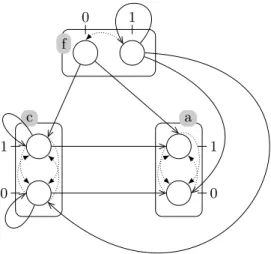
As a biologically inspired example, we propose here the model of Fig. 3 given in [9] of the metazoan segmentation network. This PH models three components containing two processes each. A controller gene f activates the two others; the products of a are responsible for a new pattern, while gene c tends to inhibit a, thus removing the pattern. This negative feedback therefore leads to a sequence of activations and inhibitions of a, creating stripes.
When applying the IG inference described in Sect. 3, we obtain the IG given in Fig. 4(left). All the edges of this inferred IG exist in the original IG of [9] which was used to produce the PH. However, an edge a −−→ a is present in+1 the original IG but is not found by our method. This can be explained by the absence of actions in the PH to model this self-influence. Furthermore, some self-influences model phenomena that impact the inferred parametrization rather than the edges of the IG (such as the action f1→ f1 f0which does not results
in a f −−→ f edge).−1
Then, the parameters inference presented in Sect. 4 allows to infer, from the input PH of Fig. 3 and inferred IG of Fig. 4(left), the parameters given in Fig. 4(right). Some of the parameters, which are signaled with an interrogation mark, could not be inferred due to contradicting influences from the regulators. For instance, in context {c0; f1}, both actions c0 → a0 a1 and f1 → a1 a0
apply and result in a cycle of bounces between a0and a1. Thus, no focal process
is found in sort a, which explains why the parameter Ka,{c},{f } is unknown. It
is interesting to notice here that the action f1 → f1 f0 previously mentioned
simply results in the parameter value Kf,∅,∅= [0; 0].
Because two parameters are impossible to infer, the original PH of Fig. 3 does not correspond to one unique BRN, but to a family of BRNs sharing the same IG but different parametrizations. This result and the method to find all admissible parametrizations of this family are given by Subsect. 4.2. As both unknown parameters can take one value amongst [0; 0], [1; 1] and [0; 1], the family contains 9 different BRNs.
By creating a cooperative sort involving f and c, it is possible to refine the dynamics and avoid the concurrent actions that prevent all parameter inferences. Such a cooperative sort is described in the reference paper, and allows to infer a complete parametrization, thus matching the original PH to a unique BRN.
f 0 1 c 0 1 a 0 1
Fig. 3. The PH model of metazoan segmentation process. This model contains three components (a, c and f ) but no cooperative sort, leading to concurrent actions on a, such as: f1→ a0 a1 and c1→ a1 a0.
c
a
f
+1 +1 −1 −1 Kf,∅,∅= [0; 0] Ka,∅,{c;f }= [0; 0] Kc,∅,{c;f }= [0; 0] Ka,{f },{c}= ? Kc,{c},{f }= [1; 1] Ka,{c},{f }= ? Kc,{f },{c}= [0; 0] Ka,{c;f },∅= [1; 1] Kc,{c;f },∅= [1; 1]Fig. 4. (left) IG inferred from the PH model of metazoan segmentation given in Fig. 3. (right) Parameters inferred from the PH model of Fig. 3 together with the (left) IG. The interrogation marks indicate parameters that could not be inferred due to the expression of opposite influences.