HAL Id: hal-00424171
https://hal.archives-ouvertes.fr/hal-00424171
Submitted on 14 Oct 2009
HAL is a multi-disciplinary open access
archive for the deposit and dissemination of
sci-entific research documents, whether they are
pub-lished or not. The documents may come from
teaching and research institutions in France or
abroad, or from public or private research centers.
L’archive ouverte pluridisciplinaire HAL, est
destinée au dépôt et à la diffusion de documents
scientifiques de niveau recherche, publiés ou non,
émanant des établissements d’enseignement et de
recherche français ou étrangers, des laboratoires
publics ou privés.
Bayesian source separation of linear-quadratic and linear
mixtures through a MCMC method
Leonardo Tomazeli Duarte, Christian Jutten, Saïd Moussaoui
To cite this version:
Leonardo Tomazeli Duarte, Christian Jutten, Saïd Moussaoui. Bayesian source separation of
linear-quadratic and linear mixtures through a MCMC method. MLSP 2009 - IEEE 19th International
Workshop on Machine Learning for Signal Processing, Sep 2009, Grenoble, France. 6 p. �hal-00424171�
BAYESIAN SOURCE SEPARATION OF LINEAR-QUADRATIC AND LINEAR MIXTURES
THROUGH A MCMC METHOD
Leonardo T. Duarte
§∗, Christian Jutten
§†and Sa¨ıd Moussaoui
‡§GIPSA-lab, UMR CNRS 5216, Institut Polytechnique de Grenoble, France
‡IRCCyN, UMR CNRS 6597, Ecole Centrale Nantes, France
{leonardo.duarte,christian.jutten}@gipsa-lab.inpg.fr, [email protected]
ABSTRACT
In this work, we deal with source separation of linear - quad-ratic (LQ) and linear mixtures. By relying on a Bayesian ap-proach, the developed method allows one to take into account prior informations such as the non-negativity and the tempo-ral structure of the sources. Concerning the inference scheme, the implementation of a Gibbs’ sampler equipped with latent variables simplifies the sampling steps. The obtained results confirm the effectiveness of the new proposal and indicate that it may be particularly useful in situations where classi-cal ICA-based solutions fail to separate the sources.
1. INTRODUCTION
In Blind Source Separation (BSS), the goal is to retrieve a set of sources by using only mixed versions of these original signals. Usually, one assumes a linear mixing process and the separation is performed via Independent Component Analysis (ICA) [1]. However, despite the notorious results provided by this classical framework, its extension to the nonlinear case is desirable as it can broaden the range of BSS applications.
Unfortunately, BSS becomes more involved in its nonlin-ear extension [2]. For example, due to the degree of flex-ibility in a nonlinear model, the application of ICA does not guarantee source separation, that is, one may recover indepen-dent components that are still mixed versions of the sources. For such reasons, a more realistic approach is to consider re-stricted classes of nonlinear models for which source separa-tion is still possible. A typical example in this context is the linear-quadratic (LQ) model [3, 4]. Besides the theoretical in-terest in the LQ model —it may pave the way for polynomial mixtures —this nonlinear model is useful in chemical sensing problems, such as in the design of gas electrode arrays [5].
Since the inversion of the LQ mixing model does not ad-mit closed formulae in the general case, a major challenge in LQ-BSS concerns the definition of a suitable structure for the separating system. In [3, 4], this problem was dealt with by defining a recurrent separating system that was trained by
∗L.T. Duarte is grateful to the CNPq (Brazil) for funding his PhD research.
†C. Jutten is with the Institut Universitaire de France.
ICA-based cost functions. Nonetheless, despite its simplic-ity and its good performance, this approach can operate only when the sources and the mixing parameters lie within the stability region of the recurrent system. Even if the develop-ment of more elaborate recurrent networks [6] can extend the stability region, it seems that the resulting training algorithms may be quite complicate in these new situations.
Motivate by the above-mentioned problems, we propose in this work a Bayesian method for separating LQ mixtures. Indeed, as the Bayesian approach treats the BSS problem rather as a data representation problem, there is no need to define a separating system in this case. Furthermore, the Bayesian framework permits us to take into account prior information other than the statistical independence. For in-stance, we consider here two prior informations that are typ-ical in chemtyp-ical sensing applications, namely: 1) the bounds of the sources and of the mixing coefficient values are known in advance, and 2) the sources have a temporal structure. It is worth mentioning that, under minor changes, the developed method can also be applied to linear models. Finally, even for the nonlinear model treated here, a simple inference scheme can be set by using a MCMC method able to simulate the posterior distributions of the parameters. In that respect, the Gibbs sampler and some auxiliary variables are employed.
Concerning the organization of the paper, we start with the mixing model description. After that, in Section 3, we present the details of our proposal. Aiming to assess the gains brought by the proposed method, a set of simulations is conducted in Section 4. Finally, we present our conclusions in Section 5.
2. MIXING MODEL
Let xi,tand sj,trepresent the i-th mixture and the j-th source
at time t, respectively. The LQ mixing model is given by
xi,t= ns X j=1 ai,jsj,t+ X 1≤j<k≤ns bi,j,ksj,tsk,t+ ni,t ∀i ∈ 1, . . . , nc, ∀t ∈ 1, . . . , nd, (1)
where ai,j et bi,j,k are the mixing parameters, and ni,t
corresponds to the noise term, which is assumed i.i.d and
Gaussian with unknown variance σ2
i. The parameters ns,
nc and nd correspond to the number of sources, sensors
and available samples, respectively. Henceforth, all the
unknown parameters will be represented by the vector1
θ = [sj,t, ai,j, bi,j,k, σi2, µj, pj], and the following
nota-tion will be adopted: θ−θq represents the vector containing
all elements of θ except θq.
3. BAYESIAN SOURCE SEPARATION METHOD In view of Eq. (1), the BSS problem treated in this work can
be put as follow: given X (matrix containing all xi,t),
esti-mate the parameters of the vector θ. In the Bayesian frame-work, this estimation task requires the expression of the poste-rior distribution p(θ|X), which, according to the Bayes’ rule, can be written as p(θ|X) ∝ p(X|θ)p(θ), where p(X|θ) is the likelihood function and p(θ) denotes the prior distribu-tions. Due to the assumption of white Gaussian noise in the observation model, the likelihood function is given by
p(X|θ) = nd Y t=1 nc Y i=1 Nxit à n s X j=1 ai,jsj,t + X 1≤j<k≤ns bi,j,ksj,tsk,t; σ2i ! , (2) where Nxik(µ; σ
2) corresponds to a Gaussian distribution of
xik with mean µ and variance σ2. The expressions of prior
distributions will be presented in the sequel. 3.1. Definition of prior distributions
3.1.1. Sources
If the limit values of the sources are known, one can incorpo-rate this information by modeling them according to a trun-cated Gaussian distribution, i.e.
p(sj,t|µj, pj, sminj , smaxj ) = q pj 2πexp ³ −pj 2 (sj,t− µj) 2´1 [smin j ,smaxj ](sj,t) Φ¡√pj ¡ smax j − µj ¢¢ − Φ¡√pj ¡ smin j − µj ¢¢ , (3)
where µj, pj are the unknown distribution parameters, and
Φ(·) is the cumulative distribution function of the standard
normal distribution. 1[smin
j ,smaxj ](sj,t) denotes the indicator
function, which takes one in the interval [smin
j , smaxj ] and
zero otherwise.
The sources usually possess a time structure in real
prob-lems. Motivated by that, a second prior modeling2 can be
1The parameters µ
jand pjcorrespond to the sources hyperparameters.
2Since the derivation of a Bayesian method is almost the same for the
i.i.d. and the Markovian modeling, our calculations will be based in Eq. (3). Note however that, in the Markovian modeling, there is no need to estimate
the term µjthat appears in this equation.
defined by substituting µj = sj,t−1 in Eq. (3). The
result-ing prior is a first-order Markovian model quite similar to the classical AR(1) model driven by Gaussian noise, with the only difference that the recurrence is limited in the interval
[smin
j , smaxj ]. Both in the i.i.d. and in the Markovian
mod-eling, we assume that the sources are mutually independent3,
i.e.4 p(S) =Qns
j=1p(sj,:).
3.1.2. Sources hyperparameters
For the i.i.d. modeling, uniform priors are assigned for the sources hyperparameters, that is
p(µj) ∝ 1[µmin
j ,µmaxj ](µj), (4)
p(pj) ∝ 1[pmin
j ,pmaxj ](pj), (5)
where the parameters µmin
j , µmaxj , pminj and pmaxj should be
assigned according to the available information. If, for ex-ample, the sources are expected to be concentrated near the
minimum value, one can set µmin
j < µmaxj < sminj .
Con-versely, if no additional information is available, one must increase the limits of both hyperparameters. Regarding the
Markovian modeling, we have only one hyperparameter (pj)
and the same prior of Eq. (5) is assigned for it.
3.1.3. Mixing parameters
Before assigning priors for the mixing parameters, let us rewrite the LQ mixing model as
xi,t= J
X
m=1
ci,m¯sm,t+ ni,t, (6)
where J = ns+2(nsns!−2)!. The vector ci = [ci,1, . . . , ci,J]
stems from the concatenation of [ai,1, . . . , ai,ns] and [bi,1,2,
. . . , bi,ns−1,ns]; and the vector ¯st = [¯s1,t, . . . , ¯sJ,t] denotes
the concatenation of the sources [s1,t, . . . , sns,t] and the linear
quadratic terms [s1,ts2,t, s2,ts3,t. . . , sns−1,tsns,t]. This new
expression points out that the conditional distributions of ai,j
and bi,j,kused in the Gibbs’ sampler (see Section 3.3) assume
similar expressions. Therefore, for sake of simplicity, both
ai,jand bi,j,kwill be represented by ci,m.
In our method, the mixing coefficients ci,m are modeled
through uniform priors, i.e.
p(ci,m) ∝1[cmin
i,m,cmaxi,m](ci,m). (7)
The distribution bounds should be set based on the available information. An interesting aspect of this modeling is that it
3As discussed in [7], for instance, the independence assumption in the
Bayesian approach is rather a working assumption, i.e., by assuming that, we are just omitting in our model a possible relation between the sources.
4In this work, c
l,m:nis an abbreviation for representing the elements
cl,m, . . . , cl,n; and cl,:represents the elements cl,1, . . . , cl,f where f is
renders possible to perform linear BSS using the same
imple-mentation of the LQ case. Indeed, if one sets cmin
i,ns+1:J =
cmax
i,ns+1:J = 0, then the parameters that multiply the
linear-quadratic terms become null, i.e. the resulting model becomes
linear. Moreover, if smin
j = 0 and smaxj → ∞, our proposal
becomes able to model non-negative prior as in non-negative matrix factorization (NMF).
3.1.4. Noise variances
A common approach [8] is to assign Gamma priors for the
noise precisions ri= 1/σi2, that is
p(ri) ∝ riαri−1exp µ −ri βri ¶ 1[0,+∞[(ri) . (8)
This choice culminates in a conjugate pair, which eases the sampling step in the Gibbs sampler. Moreover, it is
possi-ble to set the hyperparameters αri and βri to obtain a vague
prior [8].
3.2. Bayesian inference and Gibbs sampler
Since we assume that all elements of p(θ) are statistically
in-dependent (except the sources sj,:and their hyperparameters
µjand pj), the posterior distribution p(θ|X) can be rewritten
as p(θ|X) ∝ p(X|θ) × nc Y i=1 J Y m=1 p(ci,m) × ns Y n=1 p(sj,:|µj, pj) × ns Y n=1 p(µj) × ns Y n=1 p(pj) × nc Y i=1 p(σ2 i). (9)
The next step is to define an adequate algorithm for the es-timation of θ using this posterior distribution. A possible approach is based on calculating the Bayesian minimum mean square error (MMSE) estimator [9] which is defined as
θM M SE=
R
θp(θ|X)dθ.
Even though the integral present in the Bayesian MMSE estimator makes its exact calculation difficult, it is still possi-ble to obtain good solutions through approximation methods.
For example, if θ1, θ2, . . . , θM represents a set of samples
drawn from p(θ|X), then the Bayesian MMSE estimator can
be approximated by eθM M SE = M1
PM
i=1θi. Therefore, in
this methodology, which is called Monte Carlo integration, the implementation of the Bayesian MMSE estimator boils down to the task of finding an efficient way for sampling from the distribution p(θ|X).
In this work, the simulation of p(θ|X) is conducted via the Gibbs’ sampler [10], a Markov chain Monte Carlo (MCMC) method tailored to deal with high-dimensional distributions. One of the attractive features of the Gibbs’ sampler is that it permits to simulate a joint distribution by sequentially sampling from the conditional distribution of each variable. This procedure can be summarized as follows:
1. Initialize all the parameters θ0
1, θ02, . . . , θN0; 2. For p = 1 to P do θ1p ∼ p(θ1|θ2p−1, θp−13 , , . . . , θNp−1, X) θ2p ∼ p(θ2|θ1p, θ3p−1, . . . , θNp−1, X) .. . θNp ∼ p(θN|θ1p, θp2, . . . , θpN −1, X) end
The notation x ∼ p(x) stands for the sampling operation, i.e.
x is a sample obtained from the distribution p(x). Therefore,
the implementation of the Gibbs’ sampler requires the con-ditional distribution of each unknown parameter of our prob-lem. We shall obtain these expressions in the sequel.
3.3. Conditional distributions
After some manipulations, one can check that the conditional
distribution of a given parameter θqis given by
p(θq|θ−θq, X) ∝ p(X|θ)p(θq). (10)
Therefore, the calculation of the conditional distributions can be achieved by substituting the likelihood function and the prior distribution into this expression. In the sequel, this pro-cedure will be done for each unknown parameter.
3.3.1. Sources
It is not difficult to show that, by substituting expressions (2) and (3) into (10), one has
p(sj,t|θ−sj,t, X) ∝ exp " − nc X i=1 1 2σ2 i à Ψi,j,tsj,t + Ωijt !2 − 0.5pj(sj,t− µj)2 # 1[smin j ,smaxj ](sjt), (11) where Ωi,j,t= xi,t− ns X g=1,g6=j ai,gsg,t − X 1≤g<k≤ns,g6=j bi,g,ksg,tsk,t, (12) and Ψi,j,t= ai,j+ ns X g=1,g6=j bi,j,gsg,t. (13)
After expanding Eq. (11), one can obtain the expression of the conditional distribution of the sources, given by
p(sj,t|θ−sj,t, X) ∝ exp à − ¡ sj,t− µP ostj ¢2 2σ2 P ostj ! 1[smin j ,smaxj ](sj,t), (14)
where σP ostj = σ 2 Ljσ 2 j/(σ2Lj + σ 2 j) and µP ostj = (µLjσ 2 j + µjσL2j)/(σ 2 Lj+ σ 2 j), and σ2 Lj = Ãn c X i=1 Ψ2 ijt σ2 i !−1 , (15) µLj = σ 2 Lj nc X i=1 ΩijtΨijt σ2 i . (16)
The expression in (11) corresponds to a truncated Gaus-sian distribution and its simulation can be easily conducted by the procedure proposed in [11].
3.3.2. Source hyperparameters
Let us start with the derivation of the conditional distribution
of pj. As the likelihood function (2) is not a function of pj, it
asserts that p(pj|sj,:, µj) ∝ p(sj,:|, pj, µj)p(pj), that is
p(pj|sj,:, µj) ∝ p nd 2 j exp ³ − 0.5pj nd X t=1 (sj,t− µj)2 ´ × 1[pminj ,pmaxj ](pj) Φ¡√pj ¡ smax j − µj ¢¢ − Φ¡√pj ¡ smin j − µj ¢¢ . (17) This expression does not assume a standard form because of the nonlinearity in the denominator of the second term.
This is also true for the distribution p(µj|sj,:, pj) that
ap-pears in the i.i.d. modeling. These non-standard distributions could be simulated through the Metropolis-Hastings (MH) al-gorithm [10]. However, this sort of solution requires the defi-nition of an instrumental function which is usually not a trivial task. Besides, the presence of MH would increase the com-plexity of our final solution.
In an alternative approach, the use of latent variables re-sults in conditional distributions that assume standard forms. This idea, which was developed in [12], is based on the fol-lowing transformation: lj,t= µj+ p−1/2j ×Φ−1 Ã Φ¡√pj(sj,t− µj) ¢ − Φ¡√pj ¡ smin j − µj ¢¢ Φ¡√pj ¡ smax j − µj ¢¢ − Φ¡√pj ¡ smin j − µj ¢¢ ! . (18)
It can be proved [12] that if sj,tfollows a truncated Gaussian
with parameters µjand pj, then lj,tis distributed according to
a Gaussian distribution of mean µj and precision pj.
There-fore, the definition of lj,tturns the problem of estimating the
parameters of a truncated Gaussian into the one of estimating the mean and precision of a Gaussian.
From the discussion of the last paragraph, lj,t follows a
Gaussian distribution, and therefore
p(lj,:|µj, pj) = nd Y t=1 r pj 2πexp ³ −pj 2 (lj,t− µj) 2´ . (19)
Using this equation and the prior distributions (4) and (5), one
can show that the new conditional distributions of µj and pj
are given by p(µj|pj, lj,:) ∝ p(µj)p(lj,:|µj, pj) ∝1[µmin j ,µmaxj ](µj) × exp −pj· nd 2 à µj− 1 ns nd X t=1 lj,t !2 (20) p(pj|µj, lj,:) ∝ p(pj)p(lj,:|µj, pj) ∝1[pmin j ,pmaxj ](pj) × pnd2 j exp à −pj nd X t=1 (lj,t− µj)2 ! . (21)
Now we have more tractable distribution, since p(µj|pj, lj,:)
is a truncated Gaussian whereas p(pj|µj, lj,:) is a truncated
Gamma. The simulation of these two distributions can be conducted through the method proposed in [11].
The original procedure of [12], described in the last
para-graphs, can be readily extended for estimating pj when the
Markovian modeling is considered. Indeed, this can be done
by observing that the innovation process sj,t− sj,t−1 is
dis-tributed according to a truncated Gaussian whose limits de-pend on the time index. Therefore, the conditional
distribu-tion of pjin this case is obtained by substituting µj= sj,t−1
in Eq. (21). Also, the same substitution should be conducted
in Eq. (18) for the calculation of the latent variables lj,t.
3.3.3. Mixing parameters
The calculation of the conditional distributions can be done by substituting equations (7) and (2) into Eq. (10). Therefore, one obtains after some calculations
p(ci,m|θ−ci,m, X) ∝ exp
à −ρ L i,m 2 (ci,m− ν L i,m)2 ! 1[cmin
i,m,cmaxi,m](ci,m), (22)
where ρL i,m= σi2 nd X t=1 ¯ sm,t, (23) νi,mL = Pnd t=1¯sm,t ³ xi,t− PJ g=1,g6=mci,g¯sg,t ´ Pnd t=1s¯2m,t . (24) Again, the resulting conditional distribution (Eq. (22)) is a truncated Gaussian distribution and can be simulated by the technique presented in [11].
3.3.4. Noise variances
The conditional distribution of the noise precision ri= 1/σi2
gives p(ri|θ−ri, X) ∝ r nd 2 i exp (−0.5riΘi,t) rαri−1 i exp µ −ri βri ¶ 1[0,+∞[(ri) (25)
where Θi,t= xi,t−
Pns
j=1ai,jsj,t−
P
i,j,kbi,j,ksj,tsk,t. This
equation can be rewritten as
p(ri|θ−ri, X) ∝ exp µ −ri µ 0.5Θi,t+ 1 βri ¶¶ rnd2+αri−1 i 1[0,+∞[(ri) , (26)
which is a Gamma distribution with parameters αi=n2d+αri
and βi−1= 0.5Θi,t+ β−1ri .
4. RESULTS
To access the performance of our proposal, we conduct a set of simulations with synthetic data. In a first scenario, we test our method in a linear source separation problem where the sources and the mixing coefficients are non-negative. Then, we address the case of linear-quadratic mixtures. In both sit-uations, the following performance index is considered
SIR = 1 nd· ns ns X j=1 nd X t=1 10 log à E{s2 j,t} E{(sj,t− bsj,t)2} ! , (27)
where bsj,t is the estimation of the source j at time t. It is
worth remembering that bsj,tis given by bsj,t= P −B1
PP
p=Bspj,t,
where spj,trepresents the p-th sample of sj,tprovided by the
Gibbs’ sampler; P and B denotes the number of total
itera-tions and the length of the burn-in period5, respectively.
4.1. Separation of linear mixtures
To illustrate the performance of our proposal in a linear case,
we tested it in situations where nd = 300, ns = 3, nc = 3;
and the mixing matrix is given by A = [1 0.5 0.5 ; 0.6 1 0.3 ; 0.8 0.4 1] . Three scenarios were considered: 1) the sources are realizations of truncated Gaussian distributions (matched case with our i.i.d. modeling); 2) the sources are realizations of truncated Gaussian Markovian process (matched case with our Markovian modeling); 3) the sources correspond to a sine wave, a ramp function and a sawtooth wave. In all these sit-uations the signal-to-noise ratio (SNR) at each sensor was 20 dB. The total number of iterations of the Gibbs’ samples was P = 10000 with a burn-in period of B = 5000.
The results presented in Tab. 1 represent the mean SIR over 50 experiments. Despite a (not surprisingly) perfor-mance degradation when the Markovian prior is used for
5Since the Markov chain associated with the Gibbs’ sampler takes some
iterations to reach the stationary distribution, the samples generate in an ini-tial moment, the burn-in period, should be discarded.
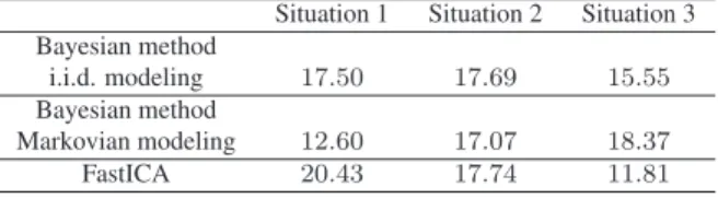
Table 1. SIR (dB) for the separation of linear mixtures.
Situation 1 Situation 2 Situation 3
Bayesian method
i.i.d. modeling 17.50 17.69 15.55
Bayesian method
Markovian modeling 12.60 17.07 18.37
FastICA 20.43 17.74 11.81
separating i.i.d. sources, our proposal was able to separate the sources. The FastICA algorithm [1] gave us better results in the first two situations. On the other hand, the application of this method on the third situation did not provide satisfac-tory results. This was due to the existence of two correlated sources in this scenario. It is worth remembering that, in contrast to the Bayesian approach, the FastICA searches for independent components and, therefore, it may fail when the sources are not independent.
4.2. Separation of linear-quadratic mixtures
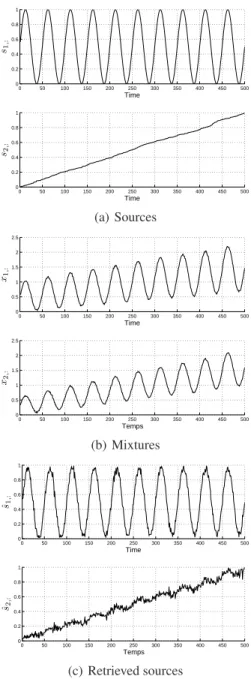
In a first moment, we considered a situation where nd = 500,
ns = 2 and nc = 2. The original sources and the mixtures
are presented in Figs. 1(a) and 1(b), respectively. The mixing
parameters were selected a1,1 = 1, a1,2 = 0.5, b1,1,2 = 0.2,
a2,1 = 0.5, a2,2 = 1, b2,1,2 = 0.2, and the SNR at each
sensor was 30 dB. The hyperparameters related to the limit
values of the prior distributions were6smin
j = cmini,m = 0 and
smax
j = cmaxi,m = 1. Concerning the Gibbs sampler
param-eters, the total number of iteration was P = 20000 with a burn in period of B = 8000. In this situation, the obtained performed index were SIR = 26.63 dB for the i.i.d. model-ing and SIR = 27.47 dB for the Markovian modelmodel-ing. We also tested the ICA method proposed in [4] which was able to provide good approximations (SIR = 22.58 dB). Despite the better performance, it worth mentioning that the gains brought by our method comes at the price of a greater com-putational effort.
We also tested our method in a second scenario simi-lar to the first one with the only difference that the
mix-ing parameters are now given by a1,1 = 1, a1,2 = 0.7,
b1,1,2 = 0.6, a2,1 = 0.6, a2,2 = 1, b2,1,2 = 0.6. Our
method was able to retrieve the sources both for i.i.d. mod-eling (SIR = 22.17 dB) and for the Markovian modmod-eling (SIR = 23.71 dB). To illustrate that, we shown in Fig. 1 the retrieved sources for the Markovian modeling. Note that, despite the noise amplification, which is typical in nonlinear systems, the retrieved signals are close to the sources. Con-versely, in this new case, the method proposed in [4] failed to separate the sources since the mixing coefficients violate the stability condition of the recurrent separating system.
6We set amin
0 50 100 150 200 250 300 350 400 450 500 0 0.2 0.4 0.6 0.8 1 Time s1 ,: 0 50 100 150 200 250 300 350 400 450 500 0 0.2 0.4 0.6 0.8 1 Time s2 ,: (a) Sources 0 50 100 150 200 250 300 350 400 450 500 0 0.5 1 1.5 2 2.5 Time x1 ,: 0 50 100 150 200 250 300 350 400 450 500 0 0.5 1 1.5 2 2.5 Temps x2 ,: (b) Mixtures 0 50 100 150 200 250 300 350 400 450 500 0 0.2 0.4 0.6 0.8 1 Time ˆs1,: 0 50 100 150 200 250 300 350 400 450 500 0 0.2 0.4 0.6 0.8 1 Temps ˆs2,: (c) Retrieved sources
Fig. 1. Separation of LQ mixtures (Markovian modeling).
5. CONCLUSION
We proposed a Bayesian source separation method that can be used in linear-quadratic and linear mixing models. The application of Gibbs’ sampler and the introduction of latent variables provided an algorithm that is easy to implement. Concerning the results, we observed that this proposal can be useful in some situations where ICA methods cannot be applied. One limitation of our solution concerns its com-putational complexity. Indeed, each iteration of the Gibbs’
sampler performs ns× ndsimulations of univariate random
variables. Therefore, the computational burden required by our proposal may become quite large in problems where the
number of sources and samples are considerable. 6. REFERENCES
[1] A. Hyv¨arinen, J. Karhunen, and E. Oja, Independent
component analysis, John Wiley & Sons, 2001.
[2] C. Jutten and J. Karhunen, “Advances in blind source
separation (BSS) and independent component analysis (ICA) for nonlinear mixtures,” International Journal of
Neural Systems, vol. 14, pp. 267–292, 2004.
[3] S. Hosseini and Y. Deville, “Blind separation of
linear-quadratic mixtures of real sources using a recurrent structure,” in Proceedings of the 7th International
Work-conference on Artificial And Natural Neural Networks, IWANN 2003, 2003, pp. 289–296.
[4] S. Hosseini and Y. Deville, “Blind maximum likelihood
separation of a linear-quadratic mixture,” in
Proceed-ings of the Fifth International Workshop on Independent Component Analysis and Blind Signal Separation, ICA 2004, 2004, pp. 694–701.
[5] G. Bedoya, Nonlinear blind signal separation for
chem-ical solid-state sensor arrays, Ph.D. thesis, Universitat
Politecnica de Catalunya, 2006.
[6] Y. Deville and S. Hosseini, “Recurrent networks for
separating extractable-target nonlinear mixtures. part i: Non-blind configurations,” Signal Processing, vol. 89, pp. 378–393, 2009.
[7] C. F´evotte and S. J. Godsill, “A bayesian approach for
blind separation of sparse sources,” IEEE Transactions
on Audio, Speech and Language Processing, vol. 14, pp.
2174–2188, 2006.
[8] S. Moussaoui, D. Brie, A. Mohammad-Djafari, and
C. Carteret, “Separation of negative mixture of non-negative sources using a Bayesian approach and MCMC sampling,” IEEE Transactions on Signal Processing, vol. 54, pp. 4133–4145, 2006.
[9] S. M. Kay, Fundamentals of statistical signal
process-ing: estimation theory, Prentice-Hall, 1993.
[10] C. P. Robert, The Bayesian Choice, Springer, 2007.
[11] P. Damien and S. G. Walker, “Sampling truncated
nor-mal, beta, and gamma densities,” Journal of
Compu-tational and Graphical Statistics, vol. 10, pp. 206–215,
2001.
[12] W. Griffiths, “A Gibbs’ sampler for a truncated
multi-variate normal distribution,” Tech. Rep., University of Melbourne, 2002.