Combining Price and Quantity Controls under Partitioned Environmental Regulation

MIT Joint Program on the Science and Policy of Global Change

combines cutting-edge scientific research with independent policy analysis to provide a solid foundation for the public and private decisions needed to mitigate and adapt to unavoidable global environmental changes. Being data-driven, the Joint Program uses extensive Earth system and economic data and models to produce quantitative analysis and predictions of the risks of climate change and the challenges of limiting human influence on the environment— essential knowledge for the international dialogue toward a global response to climate change.

To this end, the Joint Program brings together an interdisciplinary group from two established MIT research centers: the Center for Global Change Science (CGCS) and the Center for Energy and Environmental Policy Research (CEEPR). These two centers—along with collaborators from the Marine Biology Laboratory (MBL) at

Woods Hole and short- and long-term visitors—provide the united vision needed to solve global challenges.

At the heart of much of the program’s work lies MIT’s Integrated Global System Model. Through this integrated model, the program seeks to discover new interactions among natural and human climate system components; objectively assess uncertainty in economic and climate projections; critically and quantitatively analyze environmental management and policy proposals; understand complex connections among the many forces that will shape our future; and improve methods to model, monitor and verify greenhouse gas emissions and climatic impacts.

This reprint is intended to communicate research results and improve public understanding of global environment and energy challenges, thereby contributing to informed debate about climate change and the economic and social implications of policy alternatives.

—Ronald G. Prinn and John M. Reilly, Joint Program Co-Directors

MIT Joint Program on the Science and Policy

of Global Change Massachusetts Institute of Technology 77 Massachusetts Ave., E19-411 Cambridge MA 02139-4307 (USA)

T (617) 253-7492 F (617) 253-9845 globalchange@mit.edu

http://globalchange.mit.edu/ July 2016

Combining Price and Quantity Controls under

Partitioned Environmental Regulation

Combining Price and Quantity Controls under

Partitioned Environmental Regulation

Jan Abrell1_{, Sebastian Rausch}1,2

Abstract: This paper analyzes hybrid emissions trading systems (ETS) under partitioned environmental regulation when firms’ abatement costs and future emissions are uncertain. We show that hybrid policies that introduce bounds on the price or the quantity of abatement provide a way to hedge against differences in marginal abatement costs across partitions. Price bounds are more efficient than abatement bounds as they also use information on firms’ abatement technologies while abatement bounds can only address emissions uncertainty. Using a numerical stochastic optimization model with equilibrium constraints for the European carbon market, we find that introducing hybrid policies in EU ETS reduces expected excess abatement costs of achieving targeted emissions reductions under EU climate policy by up to 89 percent. We also find that under partitioned regulation there is a high likelihood for hybrid policies to yield sizeable ex-post cost reductions.

1 Department of Management, Technology, and Economics and Center for Economic Research at ETH Zurich. 2 Joint Program on the Science and Policy of Global Change, Massachusetts Institute of Technology, Cambridge, USA.

1. INTRODUCTION ... 2

2. THE THEORETICAL ARGUMENT ...4

2.1. BASIC SETUP ...4

2.2. FIRST-BEST POLICIES ...5

2.3. PURE QUANTITY CONTROLS ...5

2.4. EX-POST EFFECTS OF PRICE AND ABATEMENT BOUNDS ...5

2.5. EX-ANTE OPTIMAL POLICIES WITH PRICE BOUNDS ...7

2.6. EX-ANTE OPTIMAL POLICIES WITH ABATEMENT BOUNDS ...9

3. QUANTITATIVE FRAMEWORK FOR EMPIRICAL ANALYSIS ...10

3.1. DERIVATION OF MARGINAL ABATEMENT COST FUNCTIONS ... 10

3.2. SOURCES OF UNCERTAINTY AND SAMPLING OF MARGINAL ABATEMENT COST CURVES ...11

3.3. COMPUTATIONAL STRATEGY ... 12

4. SIMULATION RESULTS ...13

4.1. POLICY CONTEXT AND ASSUMPTIONS UNDERLYING THE SIMULATION DYNAMICS ... 13

4.2. EX-ANTE ASSESSMENT OF ALTERNATIVE HYBRID POLICY DESIGNS ... 13

4.3. IMPACTS ON EX-POST ABATEMENT COSTS ...17

5. CONCLUSION ...19

1. Introduction

Environmental regulation of an uniformly dispersed pollutant such as carbon dioxide (CO2) is often highly fragmented as regulators employ different instruments for different sources and emitters. A prominent example for partitioned environmental regulation is the Europe-an Union (EU)’s climate policy under which the overall emissions reduction target is split between sources cov-ered by the EU Emissions Trading System and sources regulated on the member state level.1

Major policy choices under partitioned environmental regulation involve choosing the instrument for each par-tition and determining how the overall environmental target is split between the partitions. Making these choic-es ex-ante, i.e. before firms’ abatement

costs and future emissions are known by the regulator, means that the ex-post marginal abatement costs will in all likelihood not be equalized across all polluting sourc-es. Given the considerable uncertainties about future abatement technologies and output (and hence emis-sions) germane to practical policymaking, partitioned environmental regulation thus inherently faces the prob-lem of achieving a given environmental target at lowest possible costs.

This paper analyzes hybrid emissions trading systems (ETS) with bounds on the price or the quantity of abate-ment when environabate-mental regulation is partitioned. We ask whether and how the ex-ante and ex-post abatement costs of partitioned climate regulation that is based on an ETS can be reduced by combining price and quantity controls. We have in mind a situation in which the regu-lator has to decide ex ante on the allocation of a given en-vironmental target between an ETS and non-ETS parti-tion and on the introducparti-tion of lower and upper bounds on the permit price or the quantity of abatement in the ETS partition. Although partitioned regulation seems to be the rule rather than the exception in the domain of real-world environmental policies, the fundamental public policy question of combining price and quantity controls—going back to the seminal contributions by Weitzman (1974) and Roberts & Spence (1976)—has so 1 The EU Emissions Trading System covers about 45% of total EU-wide emissions, mainly from electricity and energy-intensive installations. By 2020 and compared to 2005 levels, a 21% reduction in emissions has to come from sectors covered by the EU ETS and an additional 10% reduction from non-trading sectors covered by the “Effort Sharing Decision” under the EU’s “2020 Climate and Energy Package”–including transport, buildings, services, small industrial installations, and agriculture and waste. Sources not covered under the EU ETS are regulated directly by member states, often relying on renewable promotion and technology policies and other com-mand-and-control measures. Taken together, this is expected to deliv-er a reduction in EU-wide emissions of 14% relative to 2005 (which is equivalent to a 20% reduction relative to 1990 levels).

far abstracted from the important complexity of parti-tioned regulation.

The introduction of price or abatement bounds in an ETS provides a way to hedge against differences in the margin-al abatement costs across the partitions of environmentmargin-al regulation when some of the abatement burden is reallo-cated based on actual (i.e., ex-post) abatement costs. Im-portantly, this can enhance the cost-effectiveness of par-titioned environmental regulation by moving the system closer to a first-best outcome in which all emitters face identical marginal abatement costs (MACs). We theoret-ically characterize ex-ante optimal hybrid ETS policies with price or abatement bounds and show that it can be optimal to allow expected MACs to differ across sectors. We further show that from an ex-ante perspective hybrid policies can never increase the costs of partitioned envi-ronmental regulation.

We complement our theoretical analysis of hybrid pol-icies under partitioned environmental regulation with an empirical analysis of EU climate policy investigating the question to what extent introducing hybrid policies in the EU ETS could lower the costs of achieving EU’s emissions reduction goals. To this end, we develop a numerical stochastic policy optimization model with equilibrium constraints for the European carbon market that is calibrated based on empirical MAC curves de-rived from a numerical general equilibrium model. The model incorporates two important sources of firm-level uncertainties in the ETS and non-ETS sectors that are relevant for the policy design problem of carbon miti-gation: (1) uncertainty about future “no policy interven-tion” emissions, reflecting uncertain output, demand, or macroeconomic shocks, and (2) uncertainty about future abatement technologies.

We find that hybrid ETS policies yield substantial sav-ings in abatement costs relative to a pure quantity-based (i.e., the currently existing) EU ETS policy. Under sec-ond-best conditions, i.e. when the regulator can ex-an-te choose the allocation of the emissions budget across the partitions, an optimal hybrid policy reduces the ex-pected excess costs–relative to a hypothetical, first-best state-contingent policy–by up to 56% (or up to billion $1.5 per year). A third-best hybrid policy, i.e. assuming an exogenously given split of the emissions budget, that reflects current EU climate policy is found to lower ex-pected excess costs by up to 89% (or up to billion $12.1 per year). Overall, we find, however, that the ability of hybrid policies to reduce expected abatement costs di-minishes if sectoral baseline emissions exhibit a strong positive correlation. Further, we find that hybrid policies with price bounds are more effective to reduce the abate-ment costs than hybrid policies with abateabate-ment bounds. Price bounds are advantageous as they can address both

types of risks whereas abatement bounds can only hedge against emissions uncertainty.

Our quantitative analysis suggests that hybrid policies with price bounds are highly likely to yield size-able ex-post savings in abatement costs, depending on the cor-relation structure between sectoral “no intervention” emissions. If emissions are negatively (positively) cor-related, the probability of ex-post costs savings is 0.67 (0.49). Hybrid polices with abatement bounds achieve ex-post cost reductions in 66 percent of cases if baseline emissions are negatively correlated, but they yield only negligible cost savings when baseline emissions are pos-itively correlated. The reason for this is that abatement bounds fail to exploit information on firms’ abatement technology.

The present paper contributes to the existing literature in several ways. First, the paper is related to the litera-ture on ex-post efficient permit markets. As Weitzman (1974) has shown, internalizing the external effects un-der uncertainty about the costs of pollution control and damages (or benefits) from pollution will in general yield second-best outcomes with lower welfare as compared to an ex-post efficient, first-best solution. The relatively large literature on ex-post efficient permit markets has suggest-ed alternative ways for hybrid regulation strategies that combine elements of permit markets and price control (Roberts & Spence, 1976; Collinge & Oates, 1982; Unold & Requate, 2001; Newell et al., 2005). By proposing to use different institutional designs, these hybrid strategies all propose in the end to implement a price-quantity re-lation for emissions, i.e. a supply function of emissions permits, that approximates the marginal damage func-tion. The welfare gains of ex-post efficient hybrid regu-lation relative to either pure price or quantity controls have shown to be substantial (Pizer, 2002).2 _{None of the} existing studies, however, does consider the problem of combining prices and quantities under partitioned envi-ronmental regulation.

Second, a small number of recent papers examines the idea of introducing a quantity-based adjustment mecha-nism to the EU ETS (Fell, 2015; Schopp et al., 2015; Kol-lenberg & Taschini, 2015; Ellerman et al., 2015; Perino & Willner, 2015). The so-called “Market Stability Reserve (MSR)”–to be introduced in Phase 4 of the EU ETS– aims at rectifying the structural problem of allowances surplus by creating a mechanism according to which annual auction volumes are adjusted in situations where the total number of allowances in circulation is outside a 2 In a model of disaggregated firm behavior, Krysiak (2008) has shown that besides increasing expected social costs, hybrid policies can have indirect benefits due to reducing the consequences of imper-fect competition, enhancing incentives for investment, and generating a revenue for the regulating authority.

certain predefined range (EC, 2014). As long as the MSR is conceived as altering the environmental target (see, for example, Kollenberg & Taschini, 2015), it can be inter-preted as a mechanism to achieve ex-post efficiency in European carbon market.3 _{This interpretation,} howev-er, importantly depends on the premise that emissions reductions to reach the overall EU climate policy goal are allocated in a cost-effective manner across sources inside and outside the EU ETS (as generally pointed by Roberts & Spence, 1976). We contribute to this debate by analyzing a hybrid ETS when the environmental target is constant and the abatement burden has to be allocated across different partitions. Moreover, while the MSR rep-resents a quantity-based adjustment mechanism, we add by comparing the ability of price-and quantity-indexed bounds to address different types of risk.

Third, the “safety valve” literature–being in fact closely related to the original proposal made by Roberts & Spen-ce (1976)–has scrutinized the idea of introducing priSpen-ce bounds into a cap-and-trade system of emissions reg-ulation to limit the costs of meeting the cap (Jacoby & Ellerman, 2004; Pizer, 2002). Hourcade & Gershi (2002) carried this idea over into the international discussion by proposing that compliance with the Kyoto Protocol might be met by paying a “compliance penalty”. Philib-ert (2009) shows in a quantitative analysis that price caps could significantly reduce economic uncertainty stem-ming primarily from unpredictable economic growth and energy prices thus lowering the costs for global cli-mate change mitigation policy.4 _{While the “safety valve”} literature on a general level considers hybrid approach-es to emissions pricing under an ETS, it doapproach-es not place this issue in the context of partitioned environmental regulation.

Lastly, a number of studies have quantified the efficiency costs of partitioned regulation caused by limited sectoral coverage of the EU ETS (Böhringer et al., 2006, 2014) or due to strategic partitioning (Böhringer & Rosendahl, 2009; Dijkstra et al., 2011). While this literature has im-portantly contributed to informing the climate policy debate about cost-effective regulatory designs, it has ab-stracted from uncertainty and has also not investigated the issue of combining price and quantity controls. The remainder of the paper is organized as follows. Sec-tion 2 presents our theoretical argument and charac-terizes ex-ante optimal hybrid policies with price and abatement bounds under partitioned environmental reg-ulation. Section 3 describes our quantitative, empirical 3 Perino & Willner (2015), in contrast, views the MSR as being allowance preserving.

4 In fact, existing cap-and-trade systems in California, RGGI, and Australia already have introduced a price floor.

framework that we use to analyze the effects of hybrid policies for carbon mitigation in the context of EU cli-mate policy. Section 4 presents and discusses the findings from our empirical analysis. Section 5 concludes.

2. The theoretical argument

In this section, we sketch our theoretical argument for why hybrid policies which combine price and quantity controls in the context of partitioned environmental reg-ulation may decrease expected abatement costs. The ar-gument can be summarized as follows: consider an econ-omy with two polluting firms where emissions from one firm are regulated under an ETS while emissions by the other firms are regulated separately to achieve an econ-omy-wide emissions target. If the regulator is uncertain about firms’ abatement costs or future emissions, pure quantity-based regulation will fail to equalize MACs between firms in most states of the world, hence under-mining cost-effectiveness. Adding bounds on the permit price or the quantity of abatement in the ETS partition provides a hedge against too large differences in firms’ marginal abatement costs, in turn reducing the expected abatement costs of partitioned environmental regulation. 2.1. Basic setup

Although the reasoning below fits alternative applica-tions, we let climate change and CO2 abatement pol-icies guide the modeling. We have in mind a world of partitioned environmental regulation with two sets of pollution firms: one set, T, participates in an emissions trading system (ETS) while the other set, N, does not.5 We will abstract from decision making within both sets and treat T and N as one firm or sector; in particular, we assume that abatement within a sector is distributed among firms in a cost-minimizing6 _manner.

2.1.1. Firms’ abatement costs and sources of uncertainty

Firm i’s abatement costs are described by the follow-ing abatement cost function: Ci (ai, gi (ϵi)), where ai : = e0i + ϵi − ei denotes sector i’s abatement defined as the difference between the “no-intervention” baseline emissions level, e0

i + ϵi, and emissions after abatement ei. Cost functions are assumed to be increasing in abatement ( ). The functions gi denote the level of the abatement technology. We assume that gi is linear in ϵi with unitary 5 The assignment of firms to each set is fixed and exogenously given. Caillaud & Demange (2005) analyze the optimal assignment of activities to trading and tax systems.

6 The terms “firm” and ”sector” are thus used interchangeably throughout the paper.

slope ( = 1).7 _{Costs are assumed to be decreasing in the} level of the technology ( < 0). The cost functions are assumed to be strictly convex, i.e., > 0, > 0, and

> ( )2_.

ϵi is a random variable which captures all the relevant uncertainty about firms’ abatement costs. We distinguish between technology and baseline emissions uncertainty. First, technology uncertainty arises as the regulator does not know the costs associated with reducing emissions from either substituting carbon with non-carbon inputs in production or from adjusting output (or a combina-tion of both). Second, the regulator does not know the level of “no-intervention” emissions, beyond the certain level e0

i, reflecting the fact that energy demand, GDP growth, and other economic conditions may affect base-line emissions but cannot be known a priori. From the definition of abatement, it follows that baseline emissions react linearly to the signal ϵi . Technology uncertainty re-acts through the technology function gi (ϵi) on the cost function.

ϵi is distributed over compact supports

[

]

2.1.2. Policy design problem, information structure, and firm behavior

The regulator is faced with the problem of limiting economy-wide emissions at the level e ≥ ∑i ei. The ma-jor premise underlying our analysis is that regulation of emissions is partitioned: emissions from sector T only make up some fraction of total economy-wide emissions and are regulated by an ETS; sector N’s emissions are not covered by the ETS.8 _{The regulator has to split the} emissions budget across partitions by choosing sectoral emissions targets, ei. We define the allocation factor as the amount of emissions allocated to the trading sector relative to the economy-wide emissions target: λ = eT /e. A policy that only consists of λ is referred to as a pure quantity-based approach as it solely determines the quantity of permits in the ETS and maximum amount of emissions in the non-ETS sector. The central theme of this paper is to investigate hybrid policies that enlarge the instrument space by allowing to introduce, in addition to λ, lower and upper bounds on the ETS permit price (P, P) or the amount of abatement in the ETS sector (a, a). 7 gi(·) is not strictly needed for our derivations but names the

sec-ond arguments of the abatement costs function and is thus introduced for notational clarity.

8 We assume that emissions control in sector N is achieved in a cost-effective way.

The regulator’s problem is to minimize expected total abatement costs

(1)

by choosing either (1) a pure quantity-based regulation (λ), (2) hybrid regulation which combines quantity and price controls ({λ, P, P}), or (3) hybrid regulation which combines quantity control with bounds on abatement ({λ, a, a}).9

The regulator ex ante chooses a policy design, i.e. before the realizations of the random variables and hence before firms’ abatement cost and baseline emissions are known. It is assumed that the regulator is able to commit on this ex-ante announced regulatory scheme. The distribution and cost functions f and C0

i as well as baseline emissions e0

i are assumed to be “common knowledge”. Ex post, i.e. after the realizations of the random variables, firms choose their abatement. Given the price for emissions in each sector, Pi, firms choose their level of abatement by equating price with MAC, i.e. Pi = ∂Ci(ai, gi)/∂ai ∀ϵi. We assume that the environmental target is exogenous, constant, and always has to be fulfilled. Thus, if ex-ante chosen price or abatement bounds become binding ex post, sectoral emissions targets are adjusted to ensure that the economy-wide emissions target is met.

2.2. First-best policies

In an environment of complete knowledge and perfect certainty there is a formal identity between the use of prices and quantities as policy instruments. If there is any advantage to employing some forms of hybrid price and quantity control modes, therefore, it must be due to in-adequate information or uncertainty. A useful reference point is thus to define the first-best optimal policy when state-contingent policies are feasible.

The first-best quantity control, λ∗ (ϵT ,ϵN), and price con-trol, P∗ (ϵT ,ϵN), are in the form of an entire schedule and functions of the random variables ET and EN equal-izing MACs among sectors in all possible states. Thus, λ∗ (ϵT ,ϵN) and P∗ (ϵT ,ϵN) are implicitly defined by

(2)

It should be readily apparent that it is infeasible for the regulator to transmit an entire schedule of ideal price 9 As we seek to characterize (optimal) policy designs which achieve an exogenously set overall emissions target, we abstract here from explicitly including the benefits from averted pollution.

or quantity controls. A contingency message is a com-plicated, specialized contract which is expensive to draw up and hard to understand. The remainder of this paper therefore focuses on policies that cannot explicitly be made state-contingent.

2.3. Pure quantity controls

In the presence of uncertainty, price and quantity instru-ments transmit policy control in quite different ways. Before turning to hybrid price-quantity policies, we first provide some basic intuition for a pure quantity-based policy in the context of partitioned environmental regulation.

What is the ex-ante optimal allocation of the econo-my-wide emissions target among sectors if λ cannot be conditioned on ϵT and ϵN ? The optimal condition of the policy decision problem in (1) by choosing only the allo-cation factor is given as:

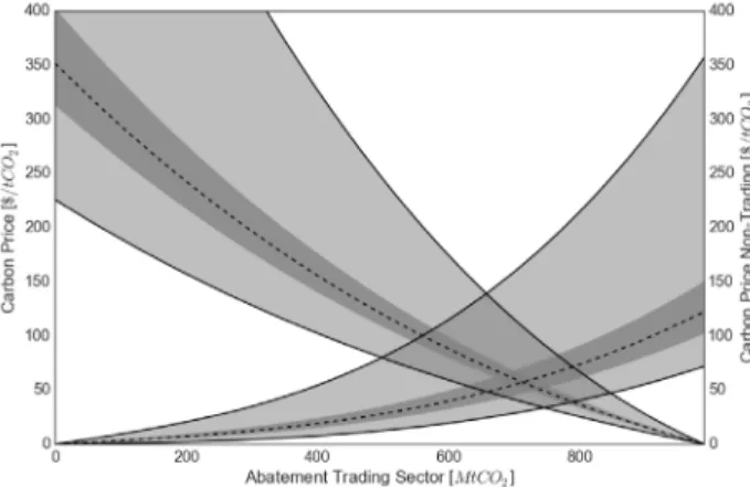
Thus, under a pure quantity approach the ex-ante opti-mal allocation factor λ∗ex-ante is chosen such that expected MACs among sectors are equalized. Given incomplete information about firms’ abatement costs and baseline emissions at the time the regulator chooses λ, in all like-lihood λ∗ex-ante ≠ λ∗ (ϵT , ϵN) which implies that MACs among sectors are not equalized ex post. Figure 1 illus-trates this situation by depicting ex-post sectoral MAC functions, λ∗ex-ante, and λ∗ (ϵT , ϵN)for a given environ-mental target. Total abatement costs are minimized if the abatement burden is partitioned according to the state-contingent policy functions λ∗ or P∗ . It is apparent from λ∗ex-ante ≠ λ∗ (ϵT , ϵN) that the realized carbon pric-es in sectors T and N, denoted, rpric-espectively, by PT and ex-ante PN differ. The excess abatement costs, i.e., change in abatement costs relative to a first-best policy with state-contingent instruments, are equal to the sum of the two gray-shaded areas in Figure 1.

Excess costs arise because of the uncertainty about firms’ abatement cost. Intuitively, ex-ante policy designs capa-ble of hedging against “too large” differences in ex-post sectoral MACs can reduce expected total abatement costs and may even lead to lower ex-post abatement costs when compared to pure quantity-based environmental regulation. This fundamental insight provides the start-ing point for investigatstart-ing hybrid policy designs. 2.4. Ex-post effects of price and abatement

bounds

To derive our results on ex ante optimal policy designs when the regulator can choose the allocation factor as

well as bounds on the permit price ({λ, P, P}) or on the level of abatement in the T sector ({λ, a, a}), it is help-ful to first develop some intuition for the possible ex-post outcomes. Consider first the case of price bounds. Given realizations of ϵT and ϵN , three cases are possible. First, if price bounds are not binding, the outcome under a hy-brid policy is identical to the one under a pure quanti-ty control. Second, the price floor binds. Given that the economy-wide emissions target is constant and has to be fulfilled, the emissions target in the T sector has to adjust downward thus shifting an equal amount of emis-sion allowances to the N sector. Third, the price ceiling binds, in which case the abatement requirement in the the T (N) sector has to decrease (increase). It is thus straightforward to see that the ex-post allocation factor is a function of the state variables ϵT and ϵN . The difference to a first-best policy is, however, that λ cannot be fully conditioned on ϵT and ϵN ; it can rather only be indirectly controlled through the ex ante choice of price bounds. To see why adding price bounds to a pure quantity-based control scheme can lower abatement costs in a sec-ond-best world, consider again Figure 1. Assume that the regulator has chosen λ∗ex-ante and a price floor P. Un-der pure quantity control (ignoring P) this would lead to the emissions prices PT and PN. If the price in the T sector realizes below the price floor (PT < P), the price bound binds with the consequence that abatement in the T sector needs to increase in order to increase the price. The abatement in the N sector therefore has to decline to ensure that the economy-wide emissions target holds, which is achieved by adjusting the allocation factor to λ.

As abatement in the N sector decreases, the carbon price in this sector declines from PN to PN. For the case depict-ed in Figure 1, the introduction of a price floor therefore moves sectoral carbon prices, and hence, sectoral MACs closer to the first-best, uniform carbon price P∗ (ϵT , ϵN). The hybrid policy therefore decreases the costs of sec-ond-best regulation by the light gray-shaded area. A sim-ilar argument can be constructed for any price ceiling above the first-best optimal emissions price.

If the regulator imposes a bound on the minimum amount of abatement, the ex post effect is similar to the one un-der a minimum permit price bound. To see this, consiun-der the case where the regulator have chosen a binding lower abatement bound such that a = e0

T λe. This triggers the same ex post adjustment in sectoral emissions budgets as with a binding price floor. Hence the savings in total abatement cost are identical. Following the same reason-ing, in Figure 1 a binding upper bound on abatement is similar to the case of a binding price ceiling.

Proposition 1. Consider an economy with polluting firms i that are partitioned in two sectors i ∈{T, N}. Sectoral abatement cost functions are strictly vex in abatement, and environmental policy is con-cerned with limiting economy-wide emissions at the level e. Each partition is regulated separately with respective targets eT and eN that are pre-determined given the allocation factor λ = eT /e. Then, intro-ducing bounds on the permit price or quantity of abatement weakly decreases economy-wide abate-ment costs

Figure 1: Abatement costs of partitioned environmental regulation under “first-best” [λ∗ (∈T ,∈N ), P∗ (∈T ,∈N )], “second-best”

(a) if the lower (upper) bound on the emissions price in one partition is smaller (greater) or equal to the optimal permit price P∗ , or

(b) if the lower (upper) bound on the amount of abatement in one partition is smaller (greater) or equal to the optimal abatement level e0

T − λ∗ e. Proof. See Appendix A.

Proposition 1 bears out a fundamental insight: under partitioned environmental regulation and given that the environmental target is fixed and always has to be met, economy-wide abatement costs cannot increase as long as the permit price floor (ceiling) is set below (above) or equal to the ex post optimal environmental tax. Consider the example of a price floor: if the initially chosen alloca-tion factor λ was too low, i.e. abatement in the ETS sector is sub-optimally high, then the permit price exceeds the optimal level but the price floor will not be binding. To-tal abatement costs will therefore not be not affected. If, however, the allocation factor was initially set too high, the ex post re-allocation of sectoral emissions targets following the introduction of a binding price floor will decrease total abatement cost. Importantly, Proposition 1 implies that in a policy environment with partitioned regulation, if the regulator has access to an estimate of the optimal permit price—or equivalently an optimal amount of abatement—in one of the sectors, a hybrid policy that introduces bounds on the permit price or on the permissible amount of abatement together with a mechanism that adjusts sectoral environmental targets under an economy-wide constant target decreases econ-omy-wide abatement costs.

2.5. Ex-ante optimal policies with price bounds

This section characterizes ex-ante optimal hybrid poli-cies with price bounds. It is useful to re-write total ex-pected abatement costs in (1) in a way that differentiates between situations in which emissions price bounds are binding or non-binding:10

(4)

where we introduced sector-specific allocation factors λi defined as λT := λ and λN = 1−λT (with equivalent defini-tions for λi and λi).

10 Throughout the analysis we assume an interior solution for λ.

The first line in (4) refers to the case when price bounds are non-binding. The second and third line refer to cases in which the price floor or ceiling is binding, respective-ly. For any ex-ante chosen λ and price bounds in sector T, there exist cutoff levels for realizations of sector T’s random variable, ϵ(λ, P) and ϵ(λ, P), at which the price floor and ceiling on the emissions price are binding. If either price bound is binding, the allocation factor has to adjust ex post to ensure that the economy-wide emissions target is achieved. These endogenous allocation factors are denoted λ(λ, P) and λ(λ, P), respectively.

The policy problem in (4) is equivalent to the one in (1) if price bounds are non-binding, i.e. the regulators could choose a price floor equal to zero and a sufficiently large price ceiling such that it never becomes binding. In such a case the expected total abatement cost function (4) is equivalent to the expected abatement cost function un-der pure quantity control (1). The regulator’s problem of choosing the policy {λ, P, P}thus includes the case of a pure quantity-based regulation.

Proposition 2. Expected total abatement costs un-der a hybrid environmental policy with emissions price bounds cannot be larger than those under pure quantity-based policy.

Proof. This follows from comparing the regulator’s policy design problems in (4) and (1) and noting that it is always possible to choose the price floor and ceiling such they are never binding. Thus, (4) is a relaxed problem of (1) and costs can never in-crease as compared to a pure quantity-based regu-lation scheme.

2.5.1. Cutoff levels and endogenous allocation factor

The hybrid policy only differs from a pure quantity control, if there exist states of the world in which price bounds are binding. We thus need to describe how the cutoff levels for the random variable in the ETS sector, ϵ(λ, P) and ϵ(λ, P), and the cutoff levels for the alloca-tion factor, λ(λ, P) and λ(λ, P) depend on policy choice variables. If the price floor is binding, cost-minimizing behavior of firms requires that marginal abatement costs equal the permit price at the bound. The lower cutoff lev-el for ϵT and λ are implicitly defined by:11

(5a)

(5b)

11 Upper cutoff levels for ∈ and λ are defined correspondingly but are not shown for reasons of brevity.

Partially differentiate (5a) and (5b) with respect to policy choice variables to obtain:12

(6a)

(6b)

(6c)

Equation (6a) reflects that a change in the (binding) price bound triggers a reallocation of abatement across sectors to hold the overall environmental target e. The magnitude of this effect depends, besides e, on the slope of the MAC curve with respect to abatement which we define as ωR > 0 or the reallocation effect. As MACs are strictly convex in abatement, it follows that ωR > 0. The steeper the MAC curve, the more the cutoff level chang-es, in turn implying a larger shift of emissions targets be-tween sectors.

Equation (6b) shows that the reaction of the cutoff lev-els for ϵ with respect to the price bounds depend on the slope of the MAC curve with respect to ϵ. Terms in brackets on the RHS indicate the change in the MAC as the threshold level changes due to affecting baseline emissions and abatement technology (i.e. through the first and second arguments of C(·)). We define the com-bined effect as the uncertainty effect, denoted by ωU . ωU is the larger, the less strongly MAC react to changes in E. The sign of ωU is ambiguous. If there is no technol-ogy uncertainty, ωU = ωR, and hence ωU > 0. With tech-nology uncertainty, and if > 0, ωU is the smaller the stronger emissions or technology uncertainty affect the MAC. A large influence of emissions uncertainty on the MAC does not necessarily mean that ωU is small as technology uncertainty can negatively impact the MAC (i.e. < 0).

Lastly, equation (6c) shows that changing λ affects the cutoff levels for ϵ in two ways. First, similar to the case 12 Changing λ has no impact on the cutoff level for λ as every change in the ex ante allocation factor is ceteris paribus compensated for by an offsetting change due to adjusting sectoral targets ex post. Thus, ∂λ/∂λ = ∂λ/∂λ = 0 is omitted from the equations below.

of a price bound, there exists an uncertainty effect. For a given change in λ, the impact on the cutoff level is the larger, the smaller is the slope of the MAC with respect to ϵ. Second, an additional reallocation effect arises because changing λ changes how the economy-wide emissions target e is allocated across sectors.

2.5.2. First-order conditions and interpretation

Expected total abatement costs are minimized when the partial derivatives in (4) with respect to λ, P, and P are zero, or when the following conditions hold:13

(7a)

(7b)

(7c)

Equation (7a) implicitly defines the ex-ante optimal fulfillment factor. Fundamentally, the optimal choice of λ still involves equating expected MACs between the two partitions. The difference compared to the case with a pure quantity control is, however, that expected margin-al costs now comprise additionmargin-al terms that reflect the marginal costs of changing λ when using price controls. The first terms on the LHS and RHS of equation (7a) rep-resent MAC for sector T and N, respectively, in the case that none of the price bounds are binding. The second and third terms reflect marginal costs from switching from an ETS system to a system of price controls.14

Proposition 3. The ex-ante optimal hybrid policy with price bounds under partitioned regulation al-locates the overall environmental target such that the expected marginal abatement costs across parti-tions differ in all likelihood in the range where price bounds are not binding.

13 See Appendix D for the derivations.

14 As for a given choice of {P, P}, the threshold levels for ∈ are known, the marginal costs under price controls are known for sector T while they are uncertain for sector N. This explains the use of expectation operators for the second and third summands on the RHS of equation (7a).

Proof. Follows from the first-order condition (7a) and noting that for a non-trivial hybrid policy, i.e. one under which there exist realizations for E such that ex-ante chosen price bounds are binding, the second and third terms on the LHS and RHS of (7a) are non-zero.

These additional terms on the LHS and RHS of equa-tion (7a) that reflect the marginal costs under a pure price-based regulation receive a higher weight if ωU /ωR ( ) is large. Intuitively, if price controls are not used, these terms (as well as the conditions in the expectation operators) drop out. Equation (7a) is then identical to the optimality condition under pure quantity control (equation (3)). With price bounds, the larger the change in the threshold levels induced by a change in the allocation factor, the higher is the weight on the margin-al cost of introducing the respective bound. The weight becomes high if the uncertainty effect is lower than the reallocation effect; by definition this implies that the change in the MAC cost due to technology uncertainty counteract the change caused by the emission uncertain-ty. In turn, there has to be a larger change in the thresh-old level implying a larger shift in the marginal cost of adjusting the allocation factor.

Equations (7b) and (7c) characterize the trade-off in choosing the optimal price floor and ceiling, respectively. Changing a price control has two effects. First, reallocat-ing abatement between sectors changes the MAC under the price regime change in both sectors (first term). The T sector’s MAC are given by the respective price control and the weighting term ωR evaluates the expected differ-ence between the price bound and the realized margin-al cost in the T sector. Second, a change in a price floor or ceiling causes a change in the threshold level. This is evaluated in the second term weighted with the marginal change of the threshold level (ωU).

2.6. Ex-ante optimal policies with abatement bounds

We now turn to the situation in which the regulator im-poses a lower (a) and upper (a) bound on the amount of abatement in the ETS sector. In this case, the objective function is similar as in the case with price bounds shown in (4).15 _{Cutoff levels for ϵ}

T and the allocation factor are again functions of policy choice variables with the differ-ence that these now depend on abatement bounds rather than on price bounds, i.e. ϵ(λ, a), ϵ(λ, a), λ(λ, a), and 15 Equation (B.5) in Appendix D states the regulator’s objective function for hybrid policies with abatement bounds.

λ(λ, a). Under a hybrid policy with abatement bounds, the cutoff levels are implicitly defined by:16

(8a)

(8b)

Taking partial derivatives of expressions for the cutoff levels for ϵ with respect to policy choice variables yields: ∂ϵ/∂λ = ∂ϵ/∂λ = e and ∂ϵ/∂a = ∂ϵ/∂a = 1. As base-line emissions uncertainty base-linearly affects abatement, a change in the allocation factor shifts the cutoff level by the same amount (taking into account that the alloca-tion factor is defined as share of the total emission level). Similarly, a change in the abatement bound changes the threshold level by the exact same amount. Policy vari-ables impact the the endogenous allocation factor as fol-lows: ∂λ/∂λ = ∂λ/∂λ = 0 and ∂λ/∂a = ∂λ/∂a = −e−1_. As in the price bound case, a change in the fulfillment factor does not affect the endogenous fulfillment factor as every change is balanced by the amount reallocated. Changing the abatement bound requires decreasing the allocation factor in order to hold the quantity balance.

Proposition 4. A hybrid policy with abatement bounds fails to exploit information on firms’ abate-ment technology when setting ex-ante minimum and maximum bounds on the permissible level of abatement.

Proof. In contrast to equations (6b)–(6c), equations (8a) and (8b) do not contain any information on the change of the MAC function.

While Proposition 4 summarizes a basic insight that is not very surprising—namely that policies aimed at tar-geting quantities rather than prices an ETS sector do not incorporate any information about the price and hence MACs of firms when determining abatement bounds—it bears out a strong implication and, in fact, foreshadows the main drawback of hybrid policies with abatement bounds when compared with policies with price bounds. Due to their ability to make use of information on firms’ (marginal) abatement costs, hybrid policies with price bounds are better suited to cope with technology uncer-tainty. While a policy with abatement bounds is able to address baseline emissions uncertainty, it is not effective in dealing with risks that affect firms’ abatement technol-ogy. In contrast, a hybrid policy with price bounds can hedge against both types of uncertainty.

16 Analogous definitions for the upper cutoff levels apply and are omitted here for brevity.

The first-order conditions for the ex-ante optimal hybrid policy with abatement bounds can be written as:17

(9a)

(9b)

(9c)

The interpretation of FOCs is similar to the case of a pol-icy with price bounds trading off the expected difference in sectoral MACs with the sum of sectoral cost changes created by introducing abatement bounds. A key differ-ence as compared to policies with price bounds is, how-ever, that as abatement bounds are not capable to infer information on the abatement cost functions and, conse-quently, do not include expected changes in the slopes of the MAC curves; all terms transporting information on firms’ abatement technology are missing.

3. Quantitative framework for

empirical analysis

We complement our theoretical analysis of hybrid poli-cies under partitioned environmental regulation with an empirical analysis of EU climate policy investigating the question to what extent introducing hybrid policies in the EU ETS could lower the costs of reaching EU’s emis-sions reductions goals. To this end, we develop and apply a stochastic policy optimization model with equilibrium constraints for the European carbon market that is cali-brated to empirically derived MAC curves.

This section describes how we operationalize the theo-retical framework presented in the previous section by (1) deriving MAC curves from a large-scale general equi-librium model of the European economy, (2) sampling MAC curves and baseline emissions for representative firms the ETS and non-ETS sectors to reflect different types of uncertainty in an empirically meaningful way, and (3) detailing our computational strategy to solve for optimal hybrid policies.

17 Appendix D contains the derivations.

3.1. Derivation of marginal abatement cost functions

Following established practice in the literature (see, for example, Klepper & Peterson, 2006; Böhringer & Rosendahl, 2009; Böhringer et al., 2014), we derive MAC curves from a multi-sector numerical general equilibri-um (GE) model of the European economy. The model structure and assumptions follow closely the GE model used in Böhringer et al. (2016).

The advantage of deriving MAC curves from a GE model is that firms’ abatement cost functions are based on firms’ equilibrium responses to a carbon price, thus reflecting both abatement through changing the input mix and the level of output while also taking into account endoge-nously determined price changes on output, factor, and intermediate input markets. By incorporating market responses on multiple layers, the derived MAC curves go beyond a pure technology-based description of firms’ abatement possibilities. The sectoral resolution further enables us to adequately represent the sectoral boundar-ies of the partitioned regulation to separately identify the MACs of sectors inside and outside of the EU ETS.

3.1.1. Overview of general equilibrium model used to derive MAC curves

We briefly highlight the key features of the numerical GE model here. Appendix C contains more detail along with a full algebraic description of the model’s equilibrium conditions. The model incorporates rich detail in ener-gy use and carbon emissions related to the combustion of fossil fuels. The energy goods identified in the model include coal, gas, crude oil, refined oil products, and elec-tricity. In addition, the model features energy-intensive sectors which are potentially most affected by carbon regulation, and other sectors (services, transportation, manufacturing, agriculture). It aggregates the EU mem-ber states into one single region.

In each region, consumption and savings result from the decisions of a continuum of identical households max-imizing utility subject to a budget constraint requiring that full consumption equals income. Households in each region receive income from two primary factors of production, capital and labor, which are supplied inelas-tically. Both factors of production are treated as perfectly mobile between sectors within a region, but not mobile between regions. All industries are characterized by con-stant returns to scale and are traded in perfectly com-petitive markets. Consumer preferences and production technologies are represented by nested constant-elastic-ity-of-substitution (CES) functions. Bilateral interna-tional trade by commodity is represented following the Armington (1969) approach where like goods produced at different locations (i.e., domestically or abroad) are

treated as imperfect substitutes. Investment demand and the foreign account balance are assumed to be fixed. A single government entity in each region approximates government activities at all levels. The government col-lects revenues from income and commodity taxation and international trade taxes. Public revenues are used to finance government consumption and (lump-sum) transfers to households. Aggregate government con-sumption combines commodities in fixed proportions. The numerical GE model makes use of a comprehensive energy-economy dataset that features a consistent rep-resentation of energy markets in physical units as well as detailed accounts of regional production and bilateral trade. Social accounting matrices in our hybrid dataset are based on data from the Global Trade Analysis Proj-ect (GTAP) (Narayanan et al., 2012). The GTAP dataset provides consistent global accounts of production, con-sumption, and bilateral trade as well as consistent ac-counts of physical energy flows and energy prices. We use the integrated economy-energy dataset to cali-brate the value share and level parameters using the stan-dard approach described in Rutherford (1998). Response parameters in the functional forms which describe production technologies and consumer preferences are determined by exogenous parameters. Table C.2 in Ap-pendix C lists the substitution elasticities and assumed parameter values in the model. Household elasticities are adopted from Paltsev et al. (2005b) and Armington trade elasticity estimates for the domestic to internation-al trade-off are taken from GTAP as estimated in Hertel et al. (2007). The remaining elasticities are own estimates consistent with the relevant literature.

3.2. Sources of uncertainty and sampling of marginal abatement cost curves

To empirically characterize uncertainty in firms’ abate-ment technology and baseline emissions, we adopt the following procedure for sampling MAC curves for the ETS and non-ETS sector.

3.2.1. Uncertainty in firms’ technology

Firms’ abatement costs depend on their production tech-nology. For each sector (or representative firm in a sec-tor), production functions are calibrated based on histor-ically observed quantities of output and inputs (capital, labor, intermediates including carbon-intensive inputs). To globally characterize CES technologies, information on elasticity of substitution (EOS) parameters are need-ed to specify second-and higher order properties of the technology. Given a calibration point, EOS parameters determine MAC curves. Unfortunately, there do not ex-ist useful estimates for EOS parameters in the literature that would characterize uncertainties involved. We

as-sume that EOS parameters for each sector are uniformly and independently distributed with a lower and upper support of, respectively, 0 and 1.5 times the central case value which we take from the literature (Narayanan et al., 2012). We then create a distribution of 10’000 MAC curves by using least squares to fit a cubic function to the price-quantity pairs sampled from 10’000 runs of the nu-merical GE model. Each run is based on a random draw of all EOS parameters from their respective distribution. For each draw, we impose a series of carbon taxes from zero to 150 $/tCO2.18

Following the design of the EU ETS, we consider electric-ity, refined oils, and energy intensive industries to be part of the trading system. All remaining sectors, including final household consumption, are subsumed under the non-trading sector. We carry out this procedure for each partition independently thereby assuming that technolo-gy shocks across sectors are uncorrelated.

3.2.2. Baseline emissions uncertainty

The distribution of baseline emissions for each sector is derived by applying the shock terms for the ETS and non-ETS sector on the respective “certain” baseline emis-sions (e0

i) as given by the numerical GE model. For our quantitative application, we have in mind the European economy around the year 2030. Assuming that baseline emissions grow with a maximum rate of ≈1% per year between 2015 and 2030, this would suggest about 15% higher emissions relative to e0

i .19

At the same time we want to allow for the possibility of reduced baseline emissions while discarding unrealisti-cally large reductions. Therefore, we assume that shocks in both sectors follow a joint truncated normal distri-bution with mean zero and a standard deviation of 5%. Lower and upper bounds for the truncation are set equal to ±15% of the baseline emissions. Shocks on sectoral baseline emissions are meant to capture both common GDP shocks, that equally affect both sectors, as well as sector-specific shocks. We thus consider alternative as-sumptions about the correlation between sectoral base-line emissions shocks; we consider three cases in which the correlation coefficient is ρ = 0, ρ = −0.5, and ρ = +0.5, respectively. Truncated normal distributions are sampled using 100’000 draws using rejection sampling (Robert & Casella, 2004).

18 We assume that the carbon revenue, net of what has to be retained to hold government spending constant in real terms, is recycled to households in a lump-sum fashion.

19 Absent any changes in energy efficiency and structural change, this would correspond to an annual average growth rate of European GDP of the same magnitude.

3.2.3. Combining uncertainties and scenario reduction

The two types of uncertainty are assumed to be indepen-dent, i.e. we assume that technology uncertainty is not af-fected by the baseline emissions uncertainty. We can thus combine the two types of uncertainty by simply adding each technology shock to any baseline emissions shock and vice versa. The size of the combined sample compris-es 1e5 _{× 1e}4 _{= 1e}9 _{observations.}

To reduce computational complexity, we employ scenar-io reductscenar-ion techniques to approximate the distributscenar-ions. Distributions for technology and baseline emissions un-certainty are approximated each using 100 points which reduces the total number of scenarios to 10’000. Approx-imation is done using k-means clustering (Hartigan & Wong, 1979) under a Euclidean distance measure and calculating centroids as means of the respective cluster. For the technology distributions, we cluster on the linear coefficient of the MAC curve and derive the mean of the higher order coefficients of the cubic MAC function af-terwards. The original and reduced distributions, along with histograms and kernel density estimates of the re-spective marginal distributions, are shown in Figures D.7 and D.8 in Appendix D.

3.3. Computational Strategy

States of the world (SOW), indexed by s, are represented by MAC curves for the ETS and non-ETS sectors, Cis, reflecting uncertainty both in firms’ abatement technolo-gy and baseline emissions. Let πs denote the probability for the occurrence of state s. Under all policies, the regu-lator minimizes expected total abatement costs

(10)

subject to an economy-wide emissions target e. ẽ0_{is ≥ 0} and eis ≥ 0 denote the level of emissions under “no inter-vention” and with policy, respectively.

3.3.1. Policies with pure quantity control The computation of first-best and second-best policies with pure quantity control is straightforward as it in-volves solving standard non-linear optimization prob-lems. Under a first-best policy, the regulator can condi-tion instruments on SOWs thereby effectively choosing ẽis. We can compute first-best policies by minimizing (10) subject to the following constraints

(11)

which ensure that the environmental target e is always met. Ps is the dual variable on this constraint and can be

interpreted as the (uniform) optimal first-best emissions permit price.

Under the second-best policy with pure quantity control, the regulator decides ex ante on the split of the econo-my-wide target between sectors, i.e. they choose sectoral targets ei ≥ 0 independent from s.

We compute second-best policies with pure quantity con-trol by minimizing (10) subject to following constraints:

(12a)

(12b)

(12a) ensures that the economy-wide target is met; the associated dual variable P is the expected permit price. (12b) ensures that emissions in each SOW are equal to the respective ex-ante chosen sectoral target. The asso-ciated dual variables are the ex-post carbon prices for each sector.

3.3.2. Hybrid policies with price and abate-ment bounds

The problem of computing ex-ante optimal hybrid pol-icies with bounds on either price or abatement falls outside the class of standard non-linear programming. The issue is that a priori it is unknown in what SOW the bounds will be binding. Cutoff levels, which define SOW in which bounds are binding, are endogenous functions of the policy choice variables. Hence, the integral bounds in the regulator’s objective function (4) are endogenous and cannot be known beforehand. We thus need to spec-ify an endogenous “rationing” mechanism that re-allo-cates emissions targets between sectors whenever one of the bounds becomes binding.

To this end, we use a complementarity-based formula-tion which explicitly represents “raformula-tioning” variables for lower and upper bounds denoted µs and µs , respectively. They appear in the following constraints s which ensure that ex-post emissions in each sector are aligned with the ex-ante emissions allocation:

(13)

where 1T(i) is an indicator variable which is equal to one if i = T and −1 otherwise.20

Condition (13) is similar to (12b) in the pure quantity con-trol case. The formulation as complementarity constraints is necessary here as it enables explicitly representing con-straint on dual variables (Pis). This allows us to formulate 20 We use the perpendicular sign ⊥� to denote complementarity, i.e., given a function F: n _{⟶ �} n_{, find z ∈�} n _{such that F(z) ≥ �0, z ≥ �0,} and zT _{F(z) = 0, or, in short-hand notation, F(z) ≥ �0 ⊥�z ≥ �0.}

policies in terms of dual variables which is needed to a rep-resentation of the hybrid policies investigated here. For the case of policies with price bounds, “rationing” variables µs and µs are determined by the following constraints:

(14a)

(14b)

As long as the price is strictly larger than the price floor, µs = 0. If the price floor becomes binding, complemen-tarity requires that µs > 0. In this case, the emissions budget in the T (N) sector decreases (increases), in turn increasing the price in the T sector.

For the case of abatement bounds, µs and µs are deter-mined by the following constraints:

(15a)

(15b)

The problem of optimal policy design can now be for-mulated as a Mathematical Program with Equilibrium Constraints (MPEC) minimizing expected abatement cost (10) subject to the emission constraints (12a), (13), and (14a) and (14b) for the case of price bounds or (15a) and (15b) for the case of abatement bounds. As MPECs are generally difficult to solve due to the lack of robust solvers (Luo et al., 1996), we reformulate the MPEC problem as a mixed complementarity problem (MCP) (Mathiesen, 1985; Rutherford, 1995) for which standard solvers exists.21 _{The MCP problem comprises} comple-mentarity conditions (13), (14a) and (14b) (for the case of price bounds), (15a) and (15b) (for the case of abate-ment bounds), and an additional condition,

(16)

which determines firms’ cost-minimizing level of abate-ment in equilibrium. To find policies that minimize (10), we perform a grid search over policy choice variables ei and (P, P) or (a, a), and compare total costs.22

21 We use the General Algebraic Modeling System (GAMS) software and the PATH solver (Dirkse & Ferris, 1995) to solve the MCP problem. We use the CONOPT solve (Drud, 1985) to solve the NLP problems when computing first-best and second-best pure quantity control policies.

22 We have used different starting values, ranges, and resolutions for the grid search to check for local optima. We find that total costs exhibit an U-shaped behavior over the policy instrument space which indicates the existence of a global cost minimum.

4. Simulation results

4.1. Policy context and assumptions underlying the simulation dynamics Our quantitative analysis seeks to approximate current EU Climate Policy. Under the “2030 Climate & Energy Framework” proposed by the European Commission (EC, 2013), it is envisaged that total EU GHG emissions are cut by at least 40% in 2030 (relative to 1990 levels). As there is still considerable uncertainty regarding the pre-cise commitment, and given that we do not model non-CO2 GHG emissions, we assume for our analysis a 30% emissions reduction target which is formulated relative to the expected value of baseline emissions.23

The “Effort Sharing Decision” under the “‘2030 Climate & Energy Package” (EC, 2008) defines reduction targets for the non-ETS sectors. We use this information to-gether with historical emissions data from the European Environment Agency to calculate an allocation factor of λˆ = .41 which determines the sectoral emissions targets under current EU climate policy.

4.2. Ex-ante assessment of alternative hybrid policy designs

We start by examining the ex-ante effects of hybrid poli-cies with price and abatement bounds under partitioned environmental regulation relative to pure quantity-based regulation. We analyze hybrid policies in the context of first-, second-, and third-best regulation. A first-best pol-icy enables choosing a state-contingent allocation factor whereas under a second-best policies an allocation factor has to be chosen ex-ante; in a third-best policy the al-location factor is exogenously given and cannot be set. We first focus on the impacts in terms of expected costs which represent the regulator’s objective. We then pro-vide insights into how alternative hybrid policies per-form under different assumptions about the type and structure of uncertainty. Finally, we analyze the potential of hybrid policies to lower expected costs in alternative third-best settings.

4.2.1. Impacts on expected costs

Table 1 presents a comparison of alternative policy de-signs under first-, second-, and third-best policy envi-ronments in terms of expected abatement costs, policy choice variables, and expected carbon prices.

Under a first-best policy which can condition the alloca-tion factor λ (or the uniform carbon price) on states of the world, the expected total abatement costs of reduc-ing European economy-wide CO2 emissions by 30% are 39.3 bill.$ with an expected carbon price of 86$/ton. 61% 23 Since we assume (∈i) = 0, (e0i + ∈i ) = e0i

of the total expected costs are borne by the ETS sector. Uncertainty increases the expected costs of regulation in second-or third-best best policy environments relative to a first-best policy: if an ex-ante optimal λ can be chosen, costs increase by 2.6 bill.$ or by about 7%; a third-best policy in which λ is exogenously given increases costs by 13.5 bill.$ or by about one third. Importantly, second-and third-best policies using a pure quantity-based approach based on λ, bring about a significantly larger variation in sectoral carbon prices as is evidenced by both lower min-imum and higher maxmin-imum ETS permit prices as well as larger standard deviations in expected carbon prices in the ETS and non-ETS sectors.

The expected excess costs of environmental regulation relative to a first-best policy are significantly reduced with hybrid policies. Under a second-best world, introducing ante optimal price bounds in the ETS reduces the ex-pected excess total abatement costs to 1.1 bill.$ which corresponds to a reduction of 56% (= (1.1/2.6 − 1) × 100) in expected excess costs relative to a first-best policy. In the third-best world, the cost reduction is particularly large. Here, a ex-ante optimal policy with price bounds reduces expected excess costs to 1.4 bill.$ which equals a 89% (= (1.4/13.5 − 1) × 100) reduction in expected

ex-cess costs relative to first-best regulation. The effects of a hybrid policies with abatement bounds on expected costs are of similar magnitudes.

The reason why second-best hybrid policies bring about sizeable reductions in expected costs of environmental regulation relative to pure quantity-based regulatory ap-proaches is that they work as a mechanism to prevent too large differences in MACs between the ETS and non-ETS sectors. This can be seen by noting that the minimum and maximum carbon prices in the ETS sector under hybrid policies in both second-and third-best cases de-scribe a more narrow range around the optimal first-best expected carbon price of 86. In addition, the standard deviation of the expected carbon price in the ETS sector decreases substantially.

In the third-best, the effectiveness of hybrid policies rests on an additional effect which stems from correcting the non-optimal allocation factor. A third-best allocation tor of λˆ = 0.41 compared to the second-best allocation fac-tor λ∗ = 0.34 means that there is too little abatement in the ETS sector (or, equivalently, an over-allocation of the emis-sions budget). By establishing a lower bound for the ETS price or the level of abatement in the ETS sector, hybrid Table 1: Comparison of expected abatement costs, allocation factor and bounds for alternative policy designs under first-, second-, and third-best policy environmentsa

First-best policy Second-best policies Third-best policies

λ∗ λ∗ λ∗ , P, P λ∗ , a, a ˆλ ˆλ, P, P ˆλ, a, a

Expected cost (bill. $/per year)

Total 39.3 41.9 40.5 40.6 52.8 40.8 40.7

ETS 24.2 25.4 24.3 24.7 11.8 24.1 24.3

Non-ETS 15.1 16.6 16.1 15.8 41.0 16.6 16.3

Ex-ante allocation factor _λ

optimal .34 .34 .33 .41 .41 .41

Carbon permit price ($/ton CO2) in ETS

min 37 21 77* 51 8 86* 54

max 197 278 101* 168 174 124* 165

Abatement (mill. ton CO2) in ETS

min 570 572 583 822** 372 617 839**

max 1’138 1’073 1’058 859** 874 997 853**

Probability that [lower,upper] price or abatement bound in ETS binds

– – [0.43,0.27] [0.35,0.5] – [0.95,0] [0.98,0]

Expected carbon price ($/ton CO2) and stdev (in parentheses)

ETS 86 (18) 89 (31) 87 (10) 88 (21) 50 (19) 86 (4) 87 (20)

Non-ETS 86 (18) 89 (37) 88 (37) 87 (32) 156 (51) 88 (41) 89 (34) Notes: λˆ denotes the “third-best” exogenous allocation factor reflecting the share of the ETS emissions budgets in total emissions based on

current EU climate policy (EC, 2008).

a _{Results shown assume negative correlation of baseline emissions shocks between sectors (ρ = −0.5).}

* Indicates ex-ante optimal floor and ceiling on ETS permit price.

polices effectively shift abatement from the non-ETS to the ETS sector. The lower price bound, set at 86$/ton, binds with a probability of 0.95; the lower bound on abatement binds with a similarly high probability of 0.98. As the mo-tive to correct the non-optimal emissions split under EU climate policy is particularly strong under the third-best case, hybrid policies work here effectively as a carbon tax. Finally, the expected costs under a third-best with price or abatement bounds are relatively close to a second-best pure quantity control policy (expected costs are only slightly lower under the second-best policy with about 1 bill.$). This result bears out an important policy impli-cation: if it is politically infeasible to correct policy deci-sions which have been taken in the past, manifested here through an exogenously given allocation factor, adding price or abatement bounds to the existing policy can achieve policy outcomes that are close to the optimum which could have been achieved under previous policy.

4.2.2. Impacts under different assumptions about uncertainty

In the absence of any uncertainty, there is no distinction between price and quantity controls, and hence no case for hybrid policies which combine elements of price and quantity control. To further investigate the performance of hybrid policies, we thus examine cases in which we switch off either type of uncertainty (i.e. baseline emis-sions or abatement technology uncertainty). In addi-tion, we analyze how the assumed correlation structure between sectoral baseline emissions shocks (ρ) affects results. Table 2 summarizes the performance of hybrid policies relative to a pure quantity control approach in terms of impacts on expected excess abatement costs24 24 See the note below Table 2 for the definition of expected ex-cess costs

for these alternative assumptions about uncertainty. Ex-pected excess abatement costs are defined as the differ-ence in expected costs relative to the first-best policy. Several insights emerge.

First, abatement bounds are completely ineffective when only technology uncertainty is present, reflecting the in-sight from Proposition 4. As ex-ante abatement bounds do not make use of firm’s marginal abatement costs, and hence information on firms’ technology, they cannot bring about reductions in expected excess abatement costs under a second-best case. It is important to un-derstand that this result only holds in the second best in which it is possible to choose an ex-ante optimal λ, in turn implying that there is no scope for abatement bounds to reduce expected costs from correcting λ. Under a third-best case, abatement bounds do indeed reduce expected costs—even if only baseline emission uncertainty is pres-ent—but this is due to correcting λˆ and not due to address-ing baseline emissions uncertainty per se. In contrast, a hybrid policy with price bounds brings about substantial cost reductions under both types of uncertainties under a second best case. If only baseline emissions uncertainty is present, price bounds, however, yield an reduction in ex-pected excess costs relative to abatement bounds because they loose their comparative advantage due to being able to address technology uncertainty.

Second, under third-best policies, price and abatement bounds yield virtually identical outcomes. The reason is simply that given a non-optimal third-best allocation factor λˆ, both types of bounds primarily work to correct λˆ. Table 2 suggests that this brings about larger reduc-tions in expected excess abatement costs than hedging against either type of uncertainty too prevent differences in sectoral MACs.

Table 2: Percentage reduction in expected excess abatement costs of hybrid policies relative to pure quantity-based regulation for alternative assumptions about uncertaintya

Second-best policies Third-best policies

(λ∗ , P, P) (λ∗ , a, a) ( ˆλ, P, P) ( ˆλ, a, a)

Correlation in sectoral baseline emissions shocks

ρ = −0.5 ρ = 0.5 ρ = −0.5 ρ = 0.5 ρ = −0.5 ρ = 0.5 ρ = −0.5 ρ = 0.5

Baseline emissions + technology uncertainty

56.4 10.2 50.3 0.2 89.3 76.1 89.8 75.1

Only baseline emissions uncertainty

63.4 0.4 63.4 0.4 93.6 78.9 93.6 78.7

Only abatement technology uncertainty

55.4 55.5 0 0 93.7 93.7 95.2 95.2 Notes: a _{Expected excess abatement costs are defined as the difference in expected costs relative to the first-best policy. Numbers above}