Probabilistic optimization of the management of corroding RC structures

HAL Id: hal-01008689

https://hal.archives-ouvertes.fr/hal-01008689

HAL is a multi-disciplinary open access archive for the deposit and dissemination of sci-entific research documents, whether they are pub-lished or not. The documents may come from teaching and research institutions in France or abroad, or from public or private research centers.

L’archive ouverte pluridisciplinaire HAL, est destinée au dépôt et à la diffusion de documents scientifiques de niveau recherche, publiés ou non, émanant des établissements d’enseignement et de recherche français ou étrangers, des laboratoires publics ou privés.

Probabilistic optimization of the management of

corroding RC structures

Emilio Bastidas-Arteaga, Franck Schoefs, Mauricio Sánchez-Silva

To cite this version:

Emilio Bastidas-Arteaga, Franck Schoefs, Mauricio Sánchez-Silva. Probabilistic optimization of the management of corroding RC structures. ASCE Structures Congress, 2011, Las Vegas, United States. �10.1061/41171(401)167�. �hal-01008689�

Probabilistic optimization of the management of corroding RC structures E. Bastidas-Arteaga1_{, F. Schoefs}1 _{and M. Sánchez-Silva}2

1_{Research Institute in Civil and Mechanical Engineering, UMR CNRS 6183,}

University of Nantes, Centrale Nantes. 2, rue de la Houssinière BP 92208 44322 Nantes Cedex 3, France; PH (+33)251125520; email: [email protected]

2_{Department of Civil and Environmental Engineering. Universidad de los Andes,}

Bogotá, Colombia ABSTRACT

This study presents a stochastic method to optimize the inspection of reinforced concrete structures subjected to chloride penetration. The strategy is oriented to find the time interval between two consecutive inspections that (1) minimize the costs of inspection, preventive and corrective repair; and (2) ensure a given level of safety. The optimal interval is therefore determined by using stochastic processes and decision theory. The chloride penetration phenomenon is represented by a Markov chain whose transition matrix is determined from simulations.

INTRODUCTION

Civil infrastructure deteriorates with time mainly as a result of environmental factors. Infrastructure deterioration may be progressive (e.g., as a result of chloride ingress), it may result from sudden events (shocks e.g., earthquakes) or as a combination of both. The cost-efficient design, management and operation of these systems depend, to a large extent, on the assumptions and quality of the deterioration models used for the analysis. Nowadays, design and management of infrastructure must consider economical, social and environmental constrains to reduce environmental impact, optimize resource allocation and decrease waste generation. This new tendency of design and management must also consider all the phenomena which affect the performance of structures. For RC structures, corrosion induced by chloride ingress generates important damage after 10 or 20 years of service (Rosquoet et al., 2006). Consequently, its inspection and maintenance are essential to ensure an optimal level of serviceability and safety during its lifespan.

The purpose of this paper is to develop a method to optimize the intervals of inspection of reinforced concrete structures subjected to chloride penetration. An optimal inspection interval minimizes the costs of inspection, preventive or corrective repair and failure. The method of optimization takes as starting point the work of Sheils et al. (2010) and is presented in the following section. Afterwards, the discussion focuses on the estimation of the transition matrices from a comprehensive model of chloride penetration and the cost modeling. Finally, the proposed methodology is illustrated with a numerical example.

STRATEGY OF INSPECTION AND MAINTENANCE

General description. Inspection can be carried out by using destructive and non-destructive methods. This study refers to RC structures subjected to chloride ingress and focuses on inspection/maintenance of major infrastructure such as ports and bridges. The requirements for the strategy of inspection/maintenance were defined within the framework of the European project FUI (2007-2010) MAREO1 with the

collaboration of public agencies, construction companies and research centers. In the strategy of inspection/maintenance considered herein, inspection is undertaken by analyzing the concentration of chlorides at the cover depth on concrete cores (destructive method). Afterwards, depending on inspection results, the repair technique consists of rebuilding the polluted concrete cover. The advantage of the proposed approach is that preventive repair ensures optimal levels of serviceability and safety during the lifespan of the project.

Inspection model. This approach requires that the structure is inspected periodically; i.e., every Δt years. The purpose of these inspections is to establish the real chloride concentration at the cover depth, C. This parameter provides information about the probability of corrosion initiation, and therefore, can be used by the owner/operator to decide if the structure must be repaired or not. The experimental test to determine the chloride profiles is based on the AFREM procedure (RILEM, 2002). Bonnet et al., (2009) found that there are significant differences between “theoretical” and “measured” chloride profiles. To take into account the influence of errors in measurement, the difference between measured Cˆ and real C values is usually

modeled by considering a noise η as follows:

η C

Cˆ= + [1]

It is supposed herein that the noise is independent of the real chloride concentration because there are several sources of error influencing the results of the inspection. This assumption has been validated from a series of measurements on metallic harbor structures (Schoefs et al. 2009).

Errors in measurement can lead to under or overestimations of chloride content, and consequently, to make erroneous decisions increasing the probability of failure or producing over-costs. From a probabilistic point of view, two measures can be defined to quantify these events:

• Probability of Good Assessment (PGA): determines the probability of detecting an event (crack, defect, concentration, etc.) given that it exists:

(

)

P ≥ ≥

= ˆ ˆ

PGA [2]

• Probability of Wrong Assessment (PWA): establishes the probability of detecting an event given that it does not exist:

(

)

P ≥ <

= ˆ ˆ

PWA [3]

where Crep represents the repair threshold. The equations presented above

assume that the noise and the signal follow a normal distribution –i.e. N[μη, ση] and

N[μ_C,σ_C].

Repair model. Chloride penetration into concrete may cause structural failure when no repair is carried out. The repair criterion considers that the polluted concrete is rebuilt when the chloride concentration measured during the inspection reaches a threshold value Cth. According to Duracrete (2000), the threshold value Cth can be

modeled by a normal distribution N[μ_Cth,σ_Cth]. Thus, the probability of corrosion initiation between the inspection intervals can be estimated as:

( )

TRANSITION MATRICES FOR MODELING CHLORIDE INGRESS

A discrete-time Markov process can be used for prediction by knowing the current state of a system. Towards this aim, the space of the variable of interest is discretized into M states. The Markov process is thus used to determine the probability that an

event belongs to a state j knowing that in a preceding state it belonged to a state i.

This probability, noted as aij=P(Xt+1= j | Xt =i), is called “transition probability”. It is

considered herein that aij is independent of t. The transition probabilities can be

grouped in a matrix of size M×M called transition matrix P. According to the

Chapman-Kolmogorov equations, by knowing an initial state, the probabilities of belonging to other states after t transitions, q(t), are (Ross, 2004):

t ini

t q P

q()= [5]

where the vector qini contains the probabilities of belonging to the states at an initial

time –i.e., t =0. In this study, the variable of interest is the concentration of chlorides

at the cover depth, C, which controls corrosion initiation. Therefore, the Markov

processes can be used to estimate the probability that C is in a given state at a given

time. If it is supposed that after construction t=0 the concentration of chlorides at the

cover depth is zero. Consequently, all the concentrations belong to the first state, qini

becomes qini=[1, 0, 0, … ,0] and equation [5] provides a vector containing the

probabilities of belonging to a state j at time t, q(t).

In several applications of Markov chains, the transition matrix is obtained from experimental data or expert judgment. However, given that the rate of chloride ingress into concrete is slow and that chloride ingress is influenced by several parameters (environment, material properties, etc.), it is proposed herein to numerically estimate q(t). The following sections will describe the adopted

probabilistic model of chloride penetration and the method proposed to estimate the transition matrix.

Chloride ingress model. Chloride ingress into concrete is controlled by a complex interaction between physical and chemical mechanisms that have been commonly modeled as a diffusion phenomenon. However, in this paper a more comprehensive

model is proposed; it considers the interaction between: (1) chloride penetration, (2) diffusion of moisture; and (3) heat transfer. The description of the formulation of the model is beyond the scope of this paper but can be found in Bastidas-Arteaga et al.,

(2011).

The management of uncertainties considers, first, the random variables presented in Table 1. The criteria for determining the characteristics of the random variables are dicussed in (Bastidas-Arteaga et al., 2011). Taking into account the

non-linearity and the complexity of the system of partial differential equations used to model chloride penetration, Monte Carlo simulations and Latin Hypercube sampling are employed herein.

Table 1. Probabilistic parameters of the random variables

Variable Units Distribution Mean COV

– Reference chloride diffusion coefficient,

Dc,ref

m2_{/s log-normal 3·10}-11 _0.20

– Activation energy of the chloride diffusion process, Uc

kJ/mol beta on [32;44.6] 41.8 0.10

– Aging factor, m beta on [0;1] 0.15 0.30

– Reference humidity diffusion coefficient, Dh,ref

m2_{/s log-normal 3·10}-10 _0.20

– Parameter representing the ratio

Dh,min/Dh,max, α0

beta on [0.025;0.1] 0.05 0.20 – Parameter characterizing the spread of

the drop in Dh, n

beta on [6;16] 11 0.10

– Thermal conductivity of concrete, λ W/(m°C) beta on [1.4;3.6] 2.5 0.20 – Specific heat capacity of concrete, cq J/(kg°C) beta on [840;1170] 1000 0.10

– Density of concrete, ρc kg/m3 Normal 2400 0.04

Estimation of the transition matrix from simulations. Transition matrices are estimated from Monte Carlo simulations of the probabilistic model of chloride penetration. In each simulation, the chloride concentration at cover depth during time is recorded. In all simulations, the frequency of belonging to a given state is determined. Thus, the probability of belonging to a state j at time t is obtained from:

N t n t q o j ) ( ) ( ˆ = [6]

where n0(t) is the number of observations in the state j measured at time t and N is

the number of simulations. Table 2 presents the possible states of the system and its corresponding boundaries (minimum and maximum); note that each state corresponds to a chloride concentration C. Taking into account this discretization,

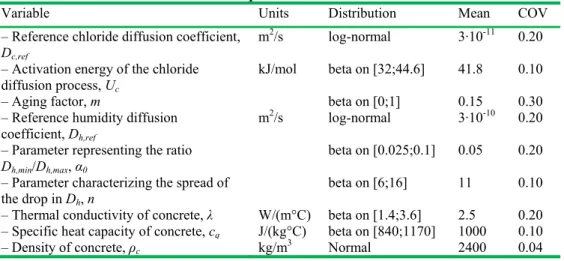
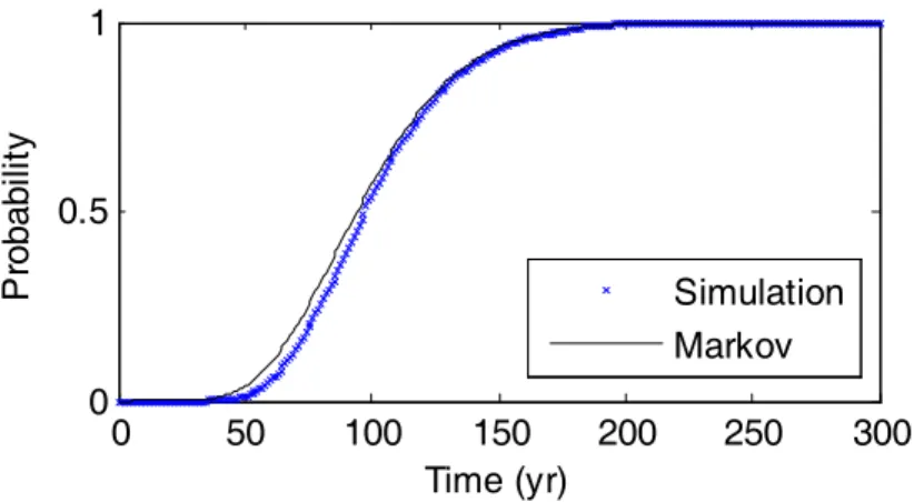
Figure 1 shows the variation in time of the probability of belonging to the last state

i=10 (qˆ t()) obtained from Monte Carlo simulations.

Table 2. States used for discretizing the problem.

State i 1 2 3 4 5 6 7 8 9 10

C minimum (kg/m3_{) 0.0 0.4 0.8 1.2 1.6 2.0 2.4 2.8 3.2 3.6}

Figure 1. Comparison between the probabilities computed from Monte Carlo simulations and Markov model for the last state.

Once the probabilities qˆ t() have been estimated, several methods can be used to compute the transition probabilities. The major difficulty in the assessment of P lies in the number of parameters aij to estimate. Various studies consider a Markov

matrix with two parameters for state (Pappas et al., 2001, Roelfstra et al., 2004). In

this case, the transition probabilities can be estimated from a non-linear regression. However, complex stochastic phenomena cannot be modeled by a transition matrix with two transition probabilities per state (Roelfstra et al. 2004). To solve this

problem, the proposed method searches the values aij that minimize the difference

between the probabilities estimated from simulations and the obtained from the Markov model (equation [5]). Since the kinematics of the time-dependent evolution of each state is similar, there are M functions to minimize:

(

)

∑

where a is a vector containing the transition probabilities (optimization parameters) and:

∑

where tana represents the analysis period used to perform the adjustment. This

multi-objective optimization problem has been solved by using the “optimization toolbox” of Matlab©. The selected optimization method minimizes the maximum value of a set of multi-variable functions from an initial value.

COST ANALYSIS

Two kinds of costs are usually considered in cost analysis: agency and user costs.

Agency costs encompass the direct costs incurred by the owner/operator during the life-cycle including initial construction costs and costs associated with inspection,

0 50 100 150 200 250 300 0 0.5 1 Time (yr) P roba bi lit y Simulation Markov

repair, rehabilitation, replacement and disposal. User costs represent the inconvenience and expenses incurred by users due to traffic disruption such as travel delay costs, ship operating costs and accident costs. According to Thoft-Christensen (2009), user costs should be included in the analysis to formulate a comprehensive strategy of maintenance management of infrastructure. However, given that the information to estimate user costs is hard to establish and find; this work is only based on agency costs.

In this study the direct costs incurred by the agency include only costs associated with maintenance (inspection, preventive repair, corrective repair and failure). The initial construction costs are not included in the analysis because it is assumed that it would be the same for all maintenance alternatives. Since it is not possible to determine the final use of the structure at the end of the life-cycle (deconstruction or demolition), the residual (or salvage) value is also not considered. This study considers costs estimated with standard and intergenerational discounting. In cycle cost analysis, the expected value of the total present value life-cycle cost E[CT] is computed as:

; for [9]

where m is the total number of interventions carried out within the time interval

[0,Tt], Cj(t) is the jth expenditure at time t (for instance in years), Tt is the life-cycle

length and W(t) is the weight used to discount Cj(t) to the present value. Cj(t)

depends on the properties of the original and repair materials; and on the characteristics of the maintenance strategy (i.e., inspection interval, inspection quality, repair threshold, etc.). The costs of inspection CI, preventive repair Cpr and

corrective repair Ccr are simply calculated as a fraction of the initial cost of

construction C0 as: I I C k C = ₀ [10] pr pr C k C = ₀ [11] cr cr C k C = ₀ [12]

where kI, kpr and kcr are weights used to compute the costs of inspection, preventive

and corrective repair as a fraction of C0, respectively.In conventional discounting, the

standard discount weight can be expressed as:

1/ 1 [13]

where rs is the standard discount rate. Sumalia and Walters (2005) and Prager and

Shertzer (2006) derived an intergenerational discount weight for computing net benefits from the use of environmental resources. In their formulation, they treat the benefits as accruing to the current generation (at standard discount rates) plus to each of the annual increments of new stakeholders who will have entered the stakeholder population by that future year divided by the generation length, G. Consequently, the

1 1

1 Δ

1 Δ

[14]

where rI is the intergenerational discount rate computed on an annual basis and Δ =

(1+rs)/(1+rI).

NUMERICAL EXAMPLE

Problem description. This example aims to determine an inspection interval that optimizes the maintenance costs of RC structures. Consider a structure placed in a marine environment with temperature ranging from 5 to 25 ºC and with relative humidity between 0.6 and 0.8. The stochastic climate model is described in (Bastidas-Arteaga et al., 2011). The structure is exposed to an average environmental chloride concentration Cenv=6 kg/m3. This concentration corresponds to the boundary

between high and severe corrosive environments (Weyers, 1994). According Duracrete, (2000), Cenv is modeled as a stochastic process generated by independent

numbers following a log-normal (log-normal noise) with a coefficient of variation of 0.2. To simplify the study, it is assumed that the repair material has the same characteristics that the construction material.

The determination of an optimal inspection interval is very sensitive to the cost models. Therefore, to obtain realistic results, the inspection, preventive repair and corrective repair coefficients (i.e., kI, kpr and kcr) were defined taking into

account the average expenditures for these items incurred by the port of Nantes Saint-Nazaire, France. These coefficients are presented in Table 3 and are used to estimate the costs of inspection, preventive and corrective repair on the basis of an initial construction cost of 1000 units. Given that it is supposed that repair is preventive, there is no failure cost and these coefficients are lower than 1. Whereas the coefficient of preventive repair only considers the cost related to cover rebuilding, the coefficient of corrective repair includes besides the costs of structural strengthening. Table 3 also includes the numerical values used to model inspection and repair.

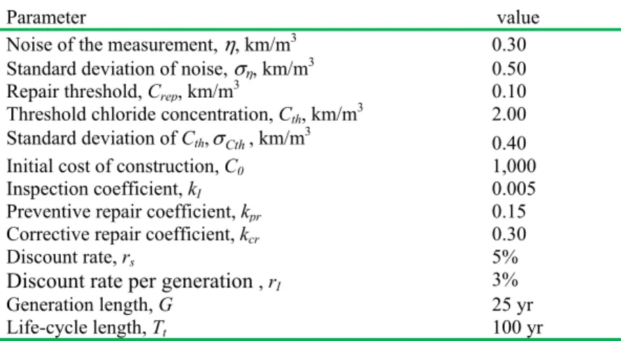
Table 3. Parameters used in the numerical example

Parameter value

Noise of the measurement, η, km/m3 _0.30

Standard deviation of noise,ση, km/m3 0.50

Repair threshold, Crep, km/m3 0.10

Threshold chloride concentration, Cth, km/m3 2.00

Standard deviation of Cth,σ , km/mCth 3 0.40

Initial cost of construction, C0 1,000

Inspection coefficient, kI 0.005

Preventive repair coefficient, kpr 0.15

Corrective repair coefficient, kcr 0.30

Discount rate, rs 5%

Discount rate per generation , rI 3%

Generation length, G 25 yr

Results. To estimate the Markov matrix, the problem is discretized into M = 10

states. The matrix P was obtained from 10,000 simulations for a concrete cover of 5cm.

Figure 1 compares the probability of belonging to the state 10 estimated by both simulations and the Markov model. Note that the phenomenon is well represented by the estimated P.

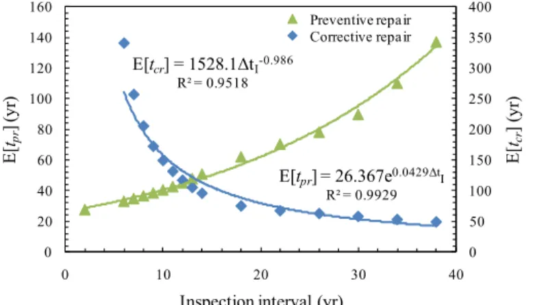
Figure 2 presents the expected times to preventive and corrective repair as a function of the length of the inspection interval. These results were obtained from the Markovian approach for a given repair technique to rebuild the concrete cover (formed concrete). As expected, the time to preventive repair, tpr, is lower when the

structure is periodically inspected. On the contrary, less inspection implies that the time to corrective repair, tcr, decreases. These times will be used to determine the

optimum inspection interval that minimizes costs. To simplify the computation, the results of simulation are adjusted to two analytical functions that will allow us to estimate tpr and tcr in terms of the length of the inspection interval ΔtI (Figure 2).

Figure 2. Determination of the expected value of the times to preventive and corrective repair

Figure 3 presents the expected costs for three cases: standard discounting, intergenerational discounting and without discounting. An intergenerational discount rate of rI = 3% (per generation) was used. The total cost is discriminated into the

costs of inspection, preventive and corrective repair. It is observed in all cases that the costs of inspection and preventive repair decrease and the cost of corrective repair increases for larger inspection intervals. This behavior is explained by the fact that when the inspection interval is greater, most inspections detect the component’s failure. On the contrary, when the structure is inspected regularly, repair is preventive, and therefore, the corrective repair expenditures diminish.

The results showed that the expected total cost is optimal when the structure is inspected every 20 years for the standard discounting case and every 15 years for the intergenerational case. However, the optimum expected cost is different for all cases because the future flows for the intergenerational and undiscounted cases are important in comparison to the standard case for the life-cycle length Tt. The

differences between the optimum inspection intervals imply that the intergenerational and undiscounted cases give more importance to preventive maintenance.

E[tpr] = 26.367e0.0429ΔtI

R² = 0.9929 E[tcr] = 1528.1ΔtI-0.986 R² = 0.9518 0 50 100 150 200 250 300 350 400 0 20 40 60 80 100 120 140 160 0 10 20 30 40 E[ tcr ] (y r) E[ tpr ] (y r)

Inspection interval (yr)

Preventive repair Corrective repair

(a) (b)

Figure 3. Expected costs for the cases (a) standard and (b) intergenerational discounting

The discount rate per generation can be defined in different ways. For instance Sumalia and Walters (2005) state that the simplest way to fix rI is to select a

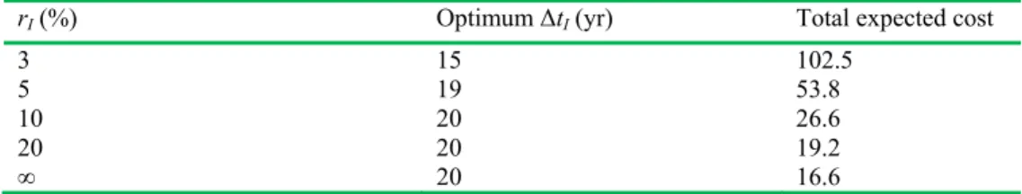
value equal to the standard discount rate. It can also be defined from a discussion with the community or it can be used the internal rate of return for educating people to the Ph.D. level in a given country. The influence of this parameter on the length of the optimum inspection interval and on the total expected cost is studied in Table 4. Therefore, for small discount rates per generation, the structure should be inspected more frequently and the total expected cost is larger. On the contrary, when rI → ∞,

the optimum result converges to the result obtained when intergenerational discounting is neglected.

Table 4. Influence of ri on the optimum inspection interval and on the total expected costs

rI (%) Optimum ΔtI (yr) Total expected cost

3 15 102.5 5 19 53.8 10 20 26.6 20 20 19.2 ∞ 20 16.6 CONCLUSIONS

This paper presents a stochastic method for optimizing the inspection/repair of RC structures subjected to chloride penetration. The inspection technique measures the concentration of chlorides at the cover depth. Afterwards, based on the inspection results, the structure is repaired by replacing the polluted concrete with new material. The inspection/maintenance strategy chosen is modeled using decision theory and Markov processes. It is also proposed a methodology for determining the transition matrix from simulations of a chloride penetration model. The proposed method is

10 20 30 40 0 20 40 60 80 100 Inspection Preventive Corrective Total Optimum

Inspection interval (yr)

Expected cost 10 20 30 40 0 50 100 150 200 Inspection Preventive Corrective Total Optimum

Inspection interval (yr)

illustrated with an example where it is showed that there is an inspection interval that minimizes the costs of inspection, preventive and corrective repair.

ACKNOWLEDGEMENTS

The authors acknowledge financial support of the MAREO project – contact: [email protected].

REFERENCES

Bastidas-Arteaga E., Chateauneuf A., Sánchez-Silva M., Bressolette P., Schoefs F. (2011). “A comprehensive probabilistic model of chloride ingress in unsaturated concrete.” Engineering Structures, In pres.

Bonnet S., Schoefs F., Ricardo J., Salta M. (2009). “Effect of error measurement of chloride profiles on reliability assessment.” Proceedings of I.C.O.S.S.A.R.,

Osaka, Japan.

Duracrete, (2000). Statistical quantification of the variables in the limit state functions. The European union, BriteEuRam III, contract BRPR-CT95-0132,

Project BE95-1347.

Pappas Y.Z., Spanos P.D., Kostopoulos V. (2001). “Markov chains for accumulation of organic and ceramic composites”. Journal of Engineering Mechanics, vol

127, pp. 915-926.

Prager, M.H. and Shertzer, K.W. (2006). Remembering the future: A commentary on “Intergenerational discounting: a new intuitive approach”. Ecological

Economics, 60:24-26.

RILEM TC178-TMC, (2002). “Analysis of chloride content in concrete.” Materials and Structures, v. 35, p. 583-585.

Roelfstra G., Hajdin R., Adey B., Brühwiler E. (2004). “Corrosion evolution in bridge management systems and corrosion-induced deterioration.”, Journal of Bridge Engineering, vol 9, pp. 268-277.

Ross S.M. (2000). Introduction to Probability models, Academic Press.

Schoefs F., Clément A., Nouy A. (2009). “Assessment of spatially dependent ROC curves for inspection of random fields of defects”, Structural Safety, v. 31,

pp. 409-419.

Sheils E., O’Connor A., Breysse D., Schoefs F., Yotte S. (2010). “Development of a two stage inspection process for the assessment of deteriorating infrastructure”, Reliability Engineering and System Safety, vol. 95, pp.

182-194.

Sumalia, U.R. and Walters, C. (2005). Intergenerational discounting: a new intuitive approach. Ecological Economics, 52:135-142.

Thoft-Christensen, P. (2009). Life-cycle cost-benefit (LCCB) analysis of bridges from a user and social point of view. Structure and Infrastructure Engineering,

5:49–57.

Weyers R.E. (1994). Concrete Bridge Protection and Rehabilitation: Chemical and Physical Techniques - Service Life Estimates. SHRP-S-668.