HAL Id: hal-00538529
https://hal.archives-ouvertes.fr/hal-00538529v2
Submitted on 1 Dec 2010
HAL is a multi-disciplinary open access
archive for the deposit and dissemination of sci-entific research documents, whether they are pub-lished or not. The documents may come from teaching and research institutions in France or abroad, or from public or private research centers.
L’archive ouverte pluridisciplinaire HAL, est destinée au dépôt et à la diffusion de documents scientifiques de niveau recherche, publiés ou non, émanant des établissements d’enseignement et de recherche français ou étrangers, des laboratoires publics ou privés.
Optimal Maintenance and Replacement Decisions under
Technological Change
Thi Phuong Khanh Nguyen, Bruno Castanier, Thomas Yeung
To cite this version:
Thi Phuong Khanh Nguyen, Bruno Castanier, Thomas Yeung. Optimal Maintenance and Replacement Decisions under Technological Change. European Safety and Reliability 2010 (ESREL 2010), Sep 2010, Greece. pp.1430-1437. �hal-00538529v2�
1 INTRODUCTION
One of the most important objectives for the main-tenance managers is to balance the mainmain-tenance ac-tion costs with the investment cost. There is an in-tensive research to provide the most appropriate strategies for organizing a set of maintenance actions generally based on complex degradation models to optimize a decision criterion. These models usually consider different maintenance actions from the “as good as new” replacement by an identical item, im-perfect maintenance which restores the item to an acceptable condition and minimal or “as bad as old” repair. They do not allow us to take into account the appearance of new technology with lower operating and maintenance costs, smaller failure rates, higher quality and output rates. This information is impor-tant for managers to decide the replacement invest-ment plan. On the other side, the models devoted to the optimization of the investment planning with the introduction of the technological change (TC) are generally based on the observations of the economi-cal performance of the maintenance process. The proposed models do not consider the diversity of maintenance decisions tackled by the deterioration-based maintenance models.
These reasons motivate us to provide an appropri-ate model to meet the operational and strappropri-ategic re-quirements. This model is developed to organize both the maintenance and replacement decisions for
a continuously deterioration system, under technolo-gical evolution.
Most of the references considering the influence of technology change are strictly economical-oriented (Bethuyne 2002, Bean et al. 1994, Elton et al. 1976, Goldstein et al. 1986, Goldstein & Mehrez 1996, Hritoneko & Yatsenko 2007, 2008a, b, 2009, Huisman & Kort 2004Nair 1995, 1997, Ott et al. 1995, Smith et al. 2003, 2007, Rajagopalan 1999). Their approach are based more on the modeling of the maintenance process through cost functions such as evolution of the operating-maintenance cost in-stead of the traditional failure indicators such as the degradation or failure rate models. Thanks to these models, the managers can decide the best time for replacement investment of equipment under tech-nological evolution but do not consider the mainten-ance strategies as well as the impact of technology change on it.
The present work continues in the direction intro-duced by articles (Borgonovo et al. 2000, Clavareau & Labeau 2009a, b, Dogramaci & Fraiman 2004, Hopp & Nair 1994, Karsak & Tolga 1998, Michel et al. 2004, Mercier 2008) that take into account the failure characteristics of the equipment in the re-placement problem under technological develop-ment. We construct a model that allows us to decide whether to imperfectly maintain, to replace with a higher technology model currently available on the
Optimal Maintenance and Replacement Decisions under Technological
Change
P.Khanh Nguyen Thi, Thomas G. Yeung & Bruno Castanier
Ecole des Mines de Nantes/IRCCyN, 44307 Nantes, France
ABSTRACT: The requirement of equipment improvement in order to satisfy the safety and reliability of sys-tem motivates the development of technology. The presence or expectation of technologically better equip-ment will influence managerial decisions on whether to invest in the maintenance of current equipequip-ment, invest in replacement with an equivalent model, replacement with a higher technology model currently available on the market, or wait for a potentially even better technology to appear in the near future. Hence, the considera-tion of technological change is a very important aspect for maintenance and replacement decisions. This paper aims to define a model that allows us to gain insight into how maintenance/replacement policies will be influ-enced by the expectation of future technology. We then use stochastic dynamic programming (i.e., Markov decision process) to solve for the optimal maintenance and replacement policy of the equipment as a function of performance and cost. Finally, we illustrate the problem through several numerical examples.
market, or wait for a potentially even better technol-ogy to appear in the near future. The technoltechnol-ogy evo-lution is modeled by a non-homogenous Poisson process and the effect of a new technology is mea-surable through the degradation characteristics. We also consider that performance of equipment in use will stochastically degrade over time due to deteri-oration while its accrued profit and maintenance cost will stochastically decrease and increase respective-ly. The objective of this paper is to maximize nue over a given planning period horizon. The reve-nue is defined here as the difference of the incomes and the outcomes. The incomes are the profit, a function of the associated degradation level, and the salvage value in case of replacement which is in-creasing in the expected mean residual life and pro-portional to the purchase price of new identical item. The outcomes are the different maintenance costs and the purchase price in case of replacement with a new technology. A discrete time non-stationary Markov Decision Process (MDP) formulation is proposed to determine the optimal action plan.
This paper is structured as follows: In Section 2, a related literature is presented to motivate the present work. Section 3 is devoted to the mathematical for-mulation. In Section 4, the performance of our mod-el is discussed through numerical examples. Finally, a conclusion and future work are discussed in Sec-tion 5.
2 RELATED LITERATURE
There are few articles that consider the maintenance – replacement problem under technological devel-opment with degradation performance. The articles of Clavareau & Labeau (2009a, b), Michel et al. (2004), Mercier (2008) examine preventive, correc-tive replacement strategies of N identical compo-nents. However, because of the complexity of the system, they must simplify the technological evolu-tion model. They consider a single new technology that has already appeared on the market with deter-ministic parameters. These assumptions are very li-mited because the technology develops rapidly and continuously. In addition, they are interested only in finding the optimal policy to replace obsolete equipments by new type, without considering whether the replacements is necessary. In our model, to attach special importance to both the continuation and the flexibility of technological change, we sim-plify the model by examining single equipment such as articles (Borgonovo et al. 2000, Hopp & Nair 1994, Dogramaci & Fraiman 2004).
We formulate a discrete time non-stationary Mar-kov Decision Process to determine the optimal main-tenance – replacement policy. The similar model
with non-stationary technological appearance’s probability in time was proposed by Nair (1995, 1997). However, in these papers, the author only considers replacement problem, not examining deci-sion to maintenance as our model. Karsark & Tolga (1998) integrate overhaul policy into replacement problem. With geometric technological evolution model, they formulate a discrete time Markov deci-sion process to determine an optimal overhaul-replacement policy which maximizes the expected present worth over a finite horizon time. But they al-so study this problem from manager’s point of view, not taking into account failure rate or deterioration process of machines. Considering of parametric per-formance represented by a Markovian deterioration process, Hopp & Nair (1994) also utilize MDP algo-rithm to dealing the equipment replacement problem under technological change. However, recall that they only consider the equipment replacement prob-lem while our work also examines the decision of maintenance. On the other hand, unlike Hopp & Nair (1994) reviewing unique challenger, we study a technological sequence.
To model sequential technological evolution, we combine the geometric model and uncertain appari-tion model of technology. The geometric technologi-cal evolution model is presented by Borgonovo et al. (2000), Smith et al. (2003), Karsak & Tolga (1998), Hritoneko & Yatsenko (2007, 2008a, b), Bethuyne (2002). But except Borgonovo et al. (2000), the rest study the problem without parametric degradation. They utilize the geometric model to form the cost functions in vintage equipment or in time. Unlike these articles, we present technology change by the improvement of the expected deterioration rate. Moreover, our profit or maintenance cost functions are only dependent on degradation state. As the ex-pected degradation rate of equipments is improved over technology generation, accrued profit and main-tenance cost will be dependent on technology gener-ation.
In addition, we also consider non-stationary like-lihood of new technology’s apparition over time. Thereby, we overcome the disadvantages of the geometric model proposed by Borgonovo et al. (2000). In that article, the failure rate decreases ex-ponentially over time, i.e. at any time, a machine can be replaced by new one which operates better with its reliability parameters determined at that time. In reality, this assumption is unreasonable because technical characteristics of the equipment can’t al-ways be changed over time. It changes only at the concurrent instant of a new technological generation. Recall that Nair (1995, 1997) also considers the non-stationary probability of the appearance of new tech-nologies. But in his model, Nair focuses on the prob-lem of capital investment decisions due to technolo-gical change rather than physical deterioration of equipment. To simplify its exposition, he also don’t
consider salvage values while we establish the rea-sonable salvage value function which depends on its mean residual life and the purchase price of identical technology at this time.
3 MODEL FORMULATION 3.1 Maintenance problem
Consider a repairable machine that operates conti-nuously from the new state, X = 0, until a failure threshold, ζ. A machine is characterized by its ex-pected deterioration rate. In the failure state, denoted m, the machine continues to operate but unprofita-bly. To reveal the deterioration level, periodic in-spections are performed. The inspection inter-val, τ, defines the decision epochs.
We assume that only one new technology can ap-pear in a decision interval, τ. We introduce 11
k i
p , the non stationary probability that technology k+1 ap-pears in the interval τ given the latest available tech-nology at decision epoch i is k. The difference in the technologies k and k+1 is modeled by an improve-ment factor on the expected instantaneous deteriora-tion rates.
Let (x, k, j) be the system state at the beginning of the ith decision epoch with observed deterioration level x when technology j is used and the technology k, k ≥ j, is available. Then, the maintenance decisions are restricted to:
1) Do nothing (DN): The machine continues to deteriorate until next decision epoch and gene-rates a profit g(x). Note that g(x) is the accrued profit within a period, depends only on the deteri-oration state at the beginning of that period. This assumption is not very restrictive in case where the decision period is sufficiently small and the decreasing rate of the profit function in deteriora-tion state is not very fast.
2) Maintain (M) which allows to restore the ma-chine in a given deterioration level, max(0, x-d) where d models the maintenance efficiency. An increasing maintenance cost in the deterioration, cM(x), is incurred and as we assume that the
main-tenance time is negligible, then, in the next deci-sion interval, the machine deteriorates from the level x-d and generates a profit g(x-d).
3) Replace (R) the equipment with the latest available technology k. The replacement time is also negligible. The cost of such a replacement is given by the difference between the purchase price of the new machine ci,k and the salvage value
bi,j(x). The purchase price is an increasing function
of technology and decreasing over time. The sal-vage value is proportional to the purchase price of technology j and decreasing in the remaining life-time. In the ith decision period after the
replace-ment, the new machine generates a profit g(0). Note that as the deterioration rates of new tech-nological machine, the purchase price can be es-timated. This is realistic in case where the tech-nical parameters and specifications of futures designs may be know beforehand.
In case of failure, the do nothing action is still al-lowed but the profit in the next decision epoch is as-sumed to be negative g(m) < 0.
3.2 Decision criteria formulation
In this paper, we use a non-stationary MDP formula-tion to find the optimal maintenance-replacement policy to maximize the expected discounted value-to-go over the finite horizon time denoted by Vπ(s). If the last decision period is N, at decision epoch N+1, we do not make any decision and the maxi-mum expected discounted value-to-go from the deci-sion epoch N+1 over the infinite horizon is VN+1(s) =
0 (sS: state space of system).
Let Vi(x,k,j) denote the maximum expected
dis-counted value from the decision epoch i, (k ≤ i) to the last epoch N. Then, V1(s) = Vπ(s).
(x,k,j)} R (x,k,j) DM (x,k,j) {DN (x,k,j) Vi max i , i , i (1) where DNi, Mi, Ri are alternately choice to do
noth-ing, to maintain and to replace at decision epoch ith. We have: '{ , 1) '[ , ] 1 )] , ' , ' ( ) , , | , ' , ' ( [ ) ( ) , , ( k k k x x i i i j k x V j k x j k x p x g j k x DN (2) ) , }, , 0 (max{ ) ( ) , , (x k j c x DN x d k j Mi M i (3) ) , , 0 ( ) ( ) , , (x k j c, b, x DN k k Ri ik i j i (4) λ: discount factor; λ [0, 1]. 3.3 Transition probabilities
To compute the transition probabilities, we propose to discretize the deteriorating state of machine as fol-lows. Let z denote the discrete deterioration state at the beginning of the current decision period. z is the first value of NX discrete intervals of length l on [0,
ζ] (which ζ is the failure threshold of the machine). That is to say, if the deterioration state (x) at the be-ginning of current decision period belongs to the in-tervals ([0, l[, [l, 2l[, [2l, 3l[, ..., [(NX - 1)l, ζ[), we
approximate x by z {0, l, 2l, 3l ... (NX-1)l} and
when the deterioration state (x) at the beginning of current decision period is exceed the failure thre-shold (x ≥ ζ), we use m to present failure state of the
machine. The deterioration state of the machine (x) is approximated by z, z {0, l, 2l, 3l ... (NX-1)l, m}.
Then, after preventive maintenance, the deterioration state is reduced by a determined amount of deteriora-tion units d. The transideteriora-tion probability is:
' 1 ) |' ( ) , , |' , ' , ' ( j ik i x k j x k j p x x p p (5) where x’ {z, z+l, …, (NX-1)l, ζ}; k’ {k, k+1}
Recall that the deterioration state of the machine at the next decision epoch depends only on its dete-rioration state at the current epoch decision and the technological generation of this machine, denoted by pj(x’|x); and
' 1
k i
p is the appearance probability of the next technological generation (k+1) at the next deci-sion epoch (i+1) with k’ = k+1 or inversely, it is the non-appearance probability with k’= k.
dy y f x x p z z l z z j j( |' ) ( ) ' '
(6) with z, z’ {0, l, 2l, 3l … (NX-1)l} and fj(y) is theprobability density function of the deterioration process of the machine’s generation jth
within the decision period τ. Similarly,
dy y f x m p z j j( | )
( ) (7) 4 NUMERICAL EXAMPLESIn this section, we present numerical examples to il-lustrate the performance of our model.
4.1 Input parameters
4.1.1 The appearance probability of new technology We define the appearance probability of new tech-nology k+1 at decision epoch i+1, given the latest available technology at decision epoch i is k, as a time increasing function:
) 1 ( 1 1 k i k i p (8) δ is the factor that reflects the non-appearance prob-ability of next generation (k+1) at next decision epoch (i+1) when the latest available technology at the current epoch i is k and k i. The smaller δ is, the greater appearance probability is. And ε is the factor characterized the increasing rate of the ap-pearance probability of new technology over time; ie. if the technological generation k+1 is not appear at decision epoch i+1, then it can appear at the next decision epoch (i+2) with probability 1 - δε given the appearance probability of (k+1) at (i+1) is 1 - δ. We
have: δ, ε [0, 1].
4.1.2 Deterioration process
We consider the machine whose degradation process is modeled by the Gamma distribution: Gamma processes are often used to model the equipment’s degradation (Van der Weide et al. 2007, Van Noort-wijk. 2009).
In any decision period, the increments of deteri-oration Xj(i + 1) – Xj(i) are independent, identical,
and follow the stationary Gamma distribution with shape parameter αjτ (recall that τ is length of a
deci-sion period) and scale parameter β. The probability density function of the deterioration process of the machine’s generation j in decision period τ is:
x j j j j x x e f 1 ) ( ) ( (9) where β is a constant and a discussion for the im-provement of αj is given in the next paragraph.
4.1.3 Impacts of the technological evolution
As we have assumed, the technological evolution aims to improve degradation characteristics, and specifically the expected degradation rate. In case of stationary gamma processes, this expected degrada-tion rate is directly propordegrada-tional to the shape parame-ter αj. We model the impact of the technological
evolution with the following decreasing exponential geometric function: b ae j j ( 1) (10) where κ, a, b are constants; j ≥ 1.
Due to technological development, the deteriora-tion rate of the machine is improved. It is convergent to the critical value, b, but the deterioration could not be excluded. We choose arbitrarily κ, a, b such as values in Table 1.
Additionally, under technological evolution, the purchase price of a new machine is assumed to be decreasing over time and normally increasing over technological generation: 1 1 1 , 1 , i k k i c v u c (11) where c1,1 is the purchase price the first of
technolo-gical generation at the first decision epoch; v is a constant, characterizing the decrease of purchase price over time (v ≤ 1) and u is constant, characteriz-ing the change of the purchase price over technolo-gical generation. We choose arbitrarily c1,1, v, u such
as values in Table 1, then ci,k is given in Table 2.
We assume the salvage value is a function of the current purchase price of this technology at this deci-sion epoch, and the Mean Residual Lifetime (MRL).
According to the degradation assumptions, if x is the observed state, we define the MRL(x) as the expected number of decision epoch from the current decision epoch until the failure. In case of stationary gamma processes, the mean deterioration rate on a decision epoch is constant and equals to αjτ/β. Hence, we
have: ) ( ) (x x MRL j . (12) Then, we propose the following function for the sal-vage value, x ϵ [0, ζ] ))] ( exp( 1 [ ) ( , , x hc rMRL x bi j i j hc, [1 exp( r ( x))] j j i (13) h, r are constant.
4.1.4 The profit and maintenance cost function We know that the machine will operate less effi-ciently when its deterioration state is greater. There-fore, the expected accrued profit function in a deci-sion period τ is decreasing by deterioration state and the greater the deterioration state is, the faster the decreases of the profit function is. To reflect this na-ture, we use a decreasing concave function of deteri-oration state x to characterize the accrued profit.
) exp( ) ( 1 0 r r x g x g g (14) x ϵ [0, ζ]; g0, rg are constant.
On the contrary, the greater the deterioration state is, the faster the increase of the maintenance cost function is. Therefore, we use an increasing convex maintenance cost function.
) exp( ) ( 1 0 r r x c x cM c (15) x ϵ [0, ζ]; c0, rc are constant.
Table 1. The input parameters for the Example 1 Appearance
prob-ability
δ ε
0.8 0.96 Profit & Discount
factor g0 rg λ 213.2 1.2 0.8 Maintenance & Failure threshold d c0 rC ζ 1.4 3.322 0.178 20 Deterioration process β a b κ NX 2.22 3 0.4 0.4 100 Salvage value &
Purchase price
h r c1,1 v u
0.8 0.4 100 0.98 1.05
Table 2. The purchase price for the Example 1 of the technolo-gy k at decision epoch i, N = 5.
i ci,1 ci,2 ci,3 ci,4 ci,5
1 100
2 98 102.9
3 96.04 100.84 105.88
4 94.12 98.83 103.77 108.95
5 92.24 96.85 101.69 106.78 112.11
4.2 Analysis from numerical experiments 4.2.1 Basic properties of the optimal policy.
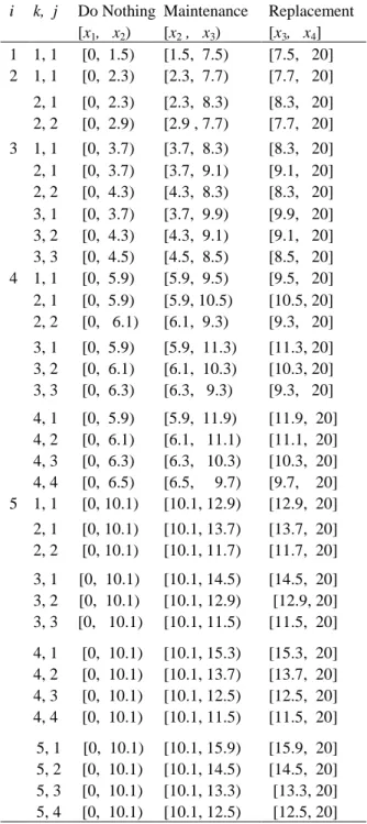
The optimal policy for the Example 1 is given in Ta-ble 3. For each decision epoch i, with the used tech-nology j, given the generation k is the latest available technology, the decision matrix defines the optimal maintenance decision according to the current dete-rioration x: Do nothing if x ϵ [x1, x2), maintain if x ϵ
[x2, x3) and replace with the new technology if x ϵ
[x3, x4].
Table 3. The optimal policy in Example 1, N = 5
i k, j Do Nothing [x1, x2) Maintenance [x2 , x3) Replacement [x3, x4] 1 1, 1 [0, 1.5) [1.5, 7.5) [7.5, 20] 2 1, 1 [0, 2.3) [2.3, 7.7) [7.7, 20] 2, 1 2, 2 [0, 2.3) [0, 2.9) [2.3, 8.3) [2.9 , 7.7) [8.3, 20] [7.7, 20] 3 1, 1 [0, 3.7) [3.7, 8.3) [8.3, 20] 2, 1 2, 2 [0, 3.7) [0, 4.3) [3.7, 9.1) [4.3, 8.3) [9.1, 20] [8.3, 20] 3, 1 3, 2 3, 3 [0, 3.7) [0, 4.3) [0, 4.5) [3.7, 9.9) [4.3, 9.1) [4.5, 8.5) [9.9, 20] [9.1, 20] [8.5, 20] 4 1, 1 [0, 5.9) [5.9, 9.5) [9.5, 20] 2, 1 2, 2 [0, 5.9) [0, 6.1) [5.9, 10.5) [6.1, 9.3) [10.5, 20] [9.3, 20] 3, 1 3, 2 3, 3 [0, 5.9) [0, 6.1) [0, 6.3) [5.9, 11.3) [6.1, 10.3) [6.3, 9.3) [11.3, 20] [10.3, 20] [9.3, 20] 4, 1 4, 2 4, 3 4, 4 [0, 5.9) [0, 6.1) [0, 6.3) [0, 6.5) [5.9, 11.9) [6.1, 11.1) [6.3, 10.3) [6.5, 9.7) [11.9, 20] [11.1, 20] [10.3, 20] [9.7, 20] 5 1, 1 [0, 10.1) [10.1, 12.9) [12.9, 20] 2, 1 2, 2 [0, 10.1) [0, 10.1) [10.1, 13.7) [10.1, 11.7) [13.7, 20] [11.7, 20] 3, 1 3, 2 3, 3 [0, 10.1) [0, 10.1) [0, 10.1) [10.1, 14.5) [10.1, 12.9) [10.1, 11.5) [14.5, 20] [12.9, 20] [11.5, 20] 4, 1 4, 2 4, 3 4, 4 [0, 10.1) [0, 10.1) [0, 10.1) [0, 10.1) [10.1, 15.3) [10.1, 13.7) [10.1, 12.5) [10.1, 11.5) [15.3, 20] [13.7, 20] [12.5, 20] [11.5, 20] 5, 1 5, 2 5, 3 5, 4 [0, 10.1) [0, 10.1) [0, 10.1) [0, 10.1) [10.1, 15.9) [10.1, 14.5) [10.1, 13.3) [10.1, 12.5) [15.9, 20] [14.5, 20] [13.3, 20] [12.5, 20]
5, 5 [0, 10.1) [10.1, 11.7) [11.7, 20]
We find that the optimal policy for Example 1, given in Table 3 has some basic properties:
1) The maintenance threshold (x2), i.e. the first
time where the optimal policy prescribes to main-tain across deterioration state x, depends only on the technological generation of the used machine j. Consider, for example, at decision epoch i = 3, the used technology j = 1, for which the optimal policy prescribes maintenance from the deteriora-tion state x2 = 3.7 despite the latest available
technology k = 1, 2, or 3. Moreover, the greater the used technology is, the higher the threshold is, because deterioration rate is improved under technological development. For example, at i = 3, k = 3, this threshold is: x2 = 3.7; 4.3; 4.5 for the
used technology j = 1, 2, 3 respectively.
2) The replacement threshold (x3) is
non-decreasing in the difference between the latest available technology and the used technology be-cause the purchase price is increasing over tech-nological generation. For example, at decision epoch i = 3, when the latest available technology is k = 3, the replacement threshold is 9.9; 9.1; 8.5 for the technology used is j = 1, 2, 3 respectively. Certainly, this threshold depends also on used technological generation (j). It is non-decreasing in the used technology j. For example, at the deci-sion epoch i = 3, when the used technology (j) is also the latest technology available (k), the re-placement threshold is 8.3; 8.3; 8.5 for j = k = 1, 2, 3 respectively.
These properties are maintained even if the finite horizon N is large enough. Consider, Example 2 with the input parameters as Example 1: the optimal poli-cy for the first three decision epochs in planning ho-rizon N = 20 is given in Table 4.
Table 4. The optimal policy for the first three decision epochs in planning horizon N = 20. i k, j Do Nothing [x1, x2) Maintenance [x2 , x3) Replacement [x3, x4] 1 1, 1 [0, 1.5) [1.5, 7.3) [7.3, 20] 2 1, 1 [0, 1.5) [1.5, 7.1) [7.1, 20] 2, 1 2, 2 [0, 1.5) [0, 1.7) [1.5, 7.3) [1.7, 7.1) [7.3, 20] [7.1, 20] 3 1, 1 [0, 1.5) [1.5, 7.1) [7.1, 20] 2, 1 2, 2 [0, 1.5) [0, 1.7) [1.5 7.1) [1.7, 7.1) [7.1, 20] [7.1, 20] 3, 1 3, 2 3, 3 [0, 1.5) [0, 1.7) [0, 1.9) [1.5, 7.5) [1.7, 7.5) [1.9, 7.3) [7.5, 20] [7.5, 20] [7.3, 20]
4.2.2 Influence of the technological improvement pa-rameter on the optimal policy
Recall that technological development is characte-rized by the improvement of the deterioration rate and the change of the purchase price ci,k. Now, we
consider the influence of these parameters on the op-timal maintenance-replacement policy.
Note that the characterization of purchase price is represented by equation: ci,k = c1,1vi-1uk-1 where u is
parameter that reflects directly the change of pur-chase price under technological development. When u > 1, the purchase price is increasing in technologi-cal generation, inversely, u < 1 this is the case where the technological improvement contributes to reduce the purchase price, and u = 1 is the case where the technological change does not influent on the pur-chase price.
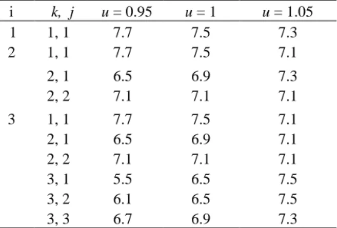
As illustrated by the numerical examples in plan-ning horizon N = 20, with u = 0.95, 1 and 1.05, con-sider the first three decision epochs (Table 5), we find that at the first decision epoch, the smaller u is, the higher the replacement threshold (x3) is. x3 = 7.7;
7.5; 7.3 respectively. The firm tends to keep the ma-chine used for waiting the appearance of new tech-nology. In the case where the new technology was available on the market, the firm tends to replace earlier when u is smaller. For example, at decision epoch i = 2, given j = 1 and k = 2, the replacement threshold is 7.3, 6.9, 6.5 for u = 1.05, 1, 0.95 respec-tively.
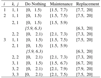
Specially, in the obsolete case, when the firms decide to replace early, the optimal policy can be non-monotone with respect to the DN and DM across deterioration x for given k, j. For example, with u = 0.95, at decision epoch i = 2, for k = 2, j = 1, the optimal policy prescribes do nothing until x = 2.5, maintain from x = 2.5 to 4.7 and then do noth-ing again at x = 4.7 until 6.5 (Table 6).
Table 5. The replacement threshold for the first three decision epochs in planning horizon N = 20 with u = 0.95; 1; 1.05
i k, j u = 0.95 u = 1 u = 1.05 1 1, 1 7.7 7.5 7.3 2 1, 1 7.7 7.5 7.1 2, 1 2, 2 6.5 7.1 6.9 7.1 7.3 7.1 3 1, 1 7.7 7.5 7.1 2, 1 2, 2 6.5 7.1 6.9 7.1 7.1 7.1 3, 1 3, 2 3, 3 5.5 6.1 6.7 6.5 6.5 6.9 7.5 7.5 7.3
Table 6. The optimal policy for the first three decision epochs in the planning horizon N = 20 with u = 0.95
i k, j Do Nothing Maintenance Replacement
1 1, 1 [0, 1.5) [1.5, 7.7) [7.7, 20] 2 1, 1 [0, 1.5) [1.5, 7.7) [7.7, 20]
2, 1 2, 2 [0, 2.5) [4.7, 6.5) [0, 1.9) [2.5, 4.7) [1.9, 7.1) [6.5, 20] [7.1, 20] 3 1, 1 [0, 1.5) [1.5, 7.7) [7.7, 20] 2, 1 2, 2 [0, 3.1) [4.1, 6.5) [0, 1.9) [6.9, 7.1) [3.1, 4.1) [1.9, 6.9) [6.5, 20] [7.1, 20] 3, 1 3, 2 3, 3 [0, 5.5) [0, 6.1) [0, 2.1) --- --- [2.1, 6.7) [5.5, 20] [6. 1, 20] [6.7, 20]
Now, we will consider how the improvement of the deterioration rate influences the optimal policy. Recall that the shape parameter of stationary Gamma function of deterioration process is represented by the decreasing exponential geometric function (equa-tion 10); where κ characterizes directly the im-provement of the deterioration rate.
We implement numerical examples in planning horizon N = 20 with κ = 0.4, 1, 1.5 and obtain the results in Table 7. We find that when j = k, the re-placement threshold is non decreasing in κ. Special-ly, at the first decision epoch, the replacement thre-shold is increasing in κ, because the firms tend to replace later for waiting the new technology when the improvement of deterioration rate is more effi-cient (κ is increasing). Consider, at i = 1, the shape parameter of the first technological generation is the same as in the case where κ = 0.4, 1, 1.5, then, the replacement threshold is 7.3, 7.5, 7.7, respectively. The case where the obsolete problem appears (j < k) is more complex. The replacement threshold is non-monotonic in κ. For example, at i = 3, the replace-ment threshold is decreasing in κ, for (k = 2, j = 1) or for (k = 3, j = 1), but it is increasing in κ for (k = 3, j = 2).
Moreover, this parameter (κ) influences also on the maintenance policy such as: the increase of the maintenance threshold (x2) in j > 1 and the
appear-ance of the non-monotone property with respect to the DN and DM across deterioration x for given k, j. As illustrated by Table 8, with κ = 1.5, at decision epoch i = 2, for k = 2, j = 1, the optimal policy pre-scribes do nothing until x2 = 1.5, maintain from x =
1.5 to 5.9 and then do nothing again from x = 5.9 to 6.3.
Table 7. The dependence of the replacement threshold on κ in planning horizon N = 20 i k, j κ = 0.4 κ =1 κ =1.5 1 1, 1 7.3 7.5 7.7 2 1, 1 7.1 7.5 7.5 2, 1 2, 2 7.3 7.1 6.5 7.3 6.3 7.3 3 1, 1 7.1 7.3 7.5 2, 1 7.1 6.5 6.3 2, 2 7.1 7.1 7.3 3, 1 3, 2 3, 3 7.5 7.5 7.3 6.9 7.7 7.5 6.7 7.9 7.5
Table 8.The optimal policy for the first three decision epochs in the planning horizon N = 20 with κ = 1.5
i k, j Do Nothing Maintenance Replacement
1 1, 1 [0, 1.5) [1.5, 7.7) [7.7, 20] 2 1, 1 [0, 1.5) [1.5, 7.5) [7.5, 20] 2, 1 2, 2 [0, 1.5) [5.9, 6.3) [0, 2.1) [1.5, 5.9) [2.1, 7.3) [6.3, 20] [7.3, 20] 3 1, 1 [0, 1.5) [1.5, 7.5) [7.5, 20] 2, 1 2, 2 [0, 1.5) [5.9, 6.3) [0, 2.1) [1.5, 5.9) [2.1, 7.3) [6.3, 20] [7.3, 20] 3, 1 3, 2 3, 3 [0, 1.5) [0, 2.1) [0, 2.1) [1.5, 6.7) [2.1, 7.9) [2.1, 7.5) [6.7, 20] [7.9, 20] [7.5, 20] 5 CONCLUSION
In this paper, we proposed a model that allows us to consider both the investment and the maintenance problem of the stochastic deterioration system under the technological development. It determines the maintenance strategy from the operator’s point of view, based on parametric performance of system. In addition, it allows the manager to take into account the necessary information of technology change to decide the best time for replacement investment of equipment as well as to consider the impact of tech-nological evolution on the maintenance strategies. We have considered a lot of assumptions and pa-rameters in our model to tackle the complexity of the decision environment for the maintenance managers. We have assumed that technological evolution is stochastic and the impact of a new technology can be measured not only from an economical point of view but also on the system deterioration performance. This high number of parameters is also due to our choice of integrating a quite well-advanced mainten-ance strategy (condition-based repair and replace-ment policy) to ensure the “local” optimality, i.e. in-dependently on the technical change opportunity, in the strategic decision context.
We then used stochastic dynamic programming (i.e., discrete non-stationary Markov decision process) to solve for the optimal maintenance and replacement policy of the equipment as a function of performance and cost. And finally, we presented numerical examples to illustrate performance of our model and to consider the influence of the parame-ters characterized the technological development on the optimal maintenance-replacement policy.
Some proposed assumptions can be seen as limita-tions of our model. The uncertainty in the technolo-gical evolution, e.g., is just considered in the time of appearance of a new generation but the associated purchase cost and the deterioration improvement are deterministic. In fact, these can be stochastic and dif-ficult to capture.
The future work could reflect the stochastic cha-racterization of these parameters. Furthermore, the stochastic efficiency of the imperfect maintenance action could also be included in our model or the conception of technology horizon N such that the initial optimal decision would be invariant even if more than N technologies wear to appear in future, could be consider .
6 REFERENCES
Bean, J.C; Lohmuann, J.R & Smith, R.L. 1994. Equipment re-placement under Technological change. Naval research
lo-gistics 41: 117-128.
Bethuyne, G. 2002. The timing of technology Adoption by a cost-minimizing firm. Journal of Economics 76: 123-154. Borgonovo, E; Marseguerra, M & Zio, E. 2000. A Monte Carlo
methodological approach to plant availability modeling with maintenance, aging and obsolescence. Reliability
Engineer-ing and System Safety 67: 61-73.
Clavareau, J & Labeau, P.E. 2009a. A Petri net-based modeling of replacement strategies under technological obsolescence.
Reliability Engineering and System Safety 94: 357- 369.
Clavareau, J & Labeau, P.E. 2009b. Maintenance and replace-ment policies under technological obsolescence. Reliability
Engineering and System Safety 94: 370-381.
Dogramaci, A & Fraiman, N.M. 2004. Replacement decisions with maintenance under uncertainty: an imbedded optimal control Model. Operations Research 52: 785-794.
Elton, E.J & Gruber, M.J. 1976. On the optimality of an equal life policy for equipment subject to technological improve-ment. Opl Res Q., Pergamon Press 27: 93-99.
Goldstein, T; Ladany,S.P & Mehrez, A. 1986. A dual machine replacement model: A Note on planning horizon procedures for machine replacements. Operations Research 34 (6): 938-941.
Goldstein, Z & Mehrez, A. 1996. Replacement of technology when a new technological breakthrough is expected. Eng.
Opt 27: 265-278.
Hopp, W.J & Nair, S.K. 1994. Maintenance and replacement policies under technological obsolescence. Reliability
Engi-neering and System Safety 94: 370-381.
Huisman, J.M & Kort, P.M. 2004. Strategic technology adop-tion taking into account future technological improvements: A real options approach. European Journal of Operational
Research 159: 705-728.
Karsak, E.E & Tolga, E. 1998. An overhaul-replacement model for equipment subject to technological change in an infla-tion-prone economy. Int. J. Production Economics 56-57: 291-301.
LoveJoy, W.S. 1987. Some monotonicity results for partially observed Markov decision processes. Operations Research 50: 796-809.
Mauer, D.C & Ott, S.H. 1995. Investment under Uncertainty: The case of replacement investment decisions. The journal
of financial and quantitative analysis 30: 581-605.
Mercier, S. 2008. Optimal replacement policy for obsolete components with general failure rates submitted to obsoles-cence. Applied Stochastic Models in Business and Industry 24: 221-235.
Michel, O; Labeau, P.E & Mercier, S. 2004. Monte Carlo op-timization of the replacement strategy of components sub-ject to technological obsolescence, Proc. of PSAM 7,
Sprin-ger 6: 282-297.
Nair, S.K. 1995. Modeling strategic investment decisions under sequential technological change. Management Science 41: 282-297.
Nair, S.K. 1997. Indentifying technology Horizons for the stra-tegic investment decisions. IEEE Transactions on
Engi-neering management 44: 227-236.
Natali, H & Yatsenko, Y. 2007. Optimal equipment replace-ment without paradoxes: A continous analysis. Operations
Research Letters 35: 245-250.
Natali, H & Yatsenko, Y. 2008b. The dynamics of asset life-time under technological change. Operations Research
Let-ter 36: 565-568.
Natali, H & Yatsenko, Y. 2008a. Properties of optimal service life under technological change. Int. J. Production
Econom-ics 114: 230-238.
Natali, H & Yatsenko, Y. 2009. Integral equation of optimal replacement: Analysis and algorithms. Applied
Mathemati-cal Modeling 33: 237-274.
Puterman. M.L. 2005. Markov decision processes – Discrete
stochastic dynamic programming. Wiley. U.S
Rajagopalan, S. 1999. Adoption timing of new equipment with another innovation anticipated. IEEE Transactions on
engi-neering management. 46: 14-25.
Schochetman, I.E & Smith, R.L. 2007. Infinite horizon opti-mality criteria for equipment replacement under technologi-cal change. Operations Research Letters 35: 485-492. Torpong, C & Smith, R.L. 2003. A paradox in equipment
re-placement under technological improvement. Operations
Research Letters 31: 77-82.
Van der Weide, J.A.M; Kallen, M.J & Pandey, M.D. 2007. Gamma process and peaks-over-threshold distributions for time-dependent reliability. Reliability Engineering and
Sys-tem Safety 92: 1651-1658.
Van Noortwijk, J.M. 2009. A survey of the application of gamma processes in maintenance. Reliability Engineering