HAL Id: hal-01100573
https://hal.archives-ouvertes.fr/hal-01100573
Submitted on 9 Jan 2015
HAL is a multi-disciplinary open access
archive for the deposit and dissemination of
sci-entific research documents, whether they are
pub-lished or not. The documents may come from
teaching and research institutions in France or
abroad, or from public or private research centers.
L’archive ouverte pluridisciplinaire HAL, est
destinée au dépôt et à la diffusion de documents
scientifiques de niveau recherche, publiés ou non,
émanant des établissements d’enseignement et de
recherche français ou étrangers, des laboratoires
publics ou privés.
extension in spatial variability -updating through
Bayesian network
Ndrianary Rakotovao Ravahatra, Thomas de Larrard, Frederic Duprat, E
Bastidas-Arteaga, Franck Schoefs
To cite this version:
Ndrianary Rakotovao Ravahatra, Thomas de Larrard, Frederic Duprat, E Bastidas-Arteaga, Franck
Schoefs. Sensitivity analysis of simplified models of carbonation extension in spatial variability
-updating through Bayesian network. Proceedings of the 2nd International Symposium on Uncertainty
Quantification and Stochastic Modeling, Jun 2014, Rouen, France. �hal-01100573�
SENSITIVITY ANALYSIS OF SIMPLIFIED MODELS OF CARBONATION
-EXTENSION IN SPATIAL VARIABILITY - UPDATING THROUGH
BAYESIAN NETWORK
N. Rakotovao Ravahatra1,2, T. de Larrard1, F. Duprat1, E. Bastidas-Arteaga2, F. Schoefs2
1University of Toulouse, UPS, INSA, LMDC (Laboratoire Materiaux et Durabilite des Constructions), 135 Avenue de Rangueil, F-31077 Toulouse Cedex 4, France
2LUNAM University, University of Nantes,Research Institute in Civil and Mechanical Engineering (GeM),UMR CNRS 6183, 2 rue de la Houssiniere, BP 92208, 44322 Nantes cedex 3, France
Abstract. The aim of this work is to handle simplified models of carbonation in a probablistic approach in order to propose an optimized maintenance strategy against steel corrosion. First of all, a synthesis of existing simplified models is presented. Three categories of models have been highlighted. Then a sensitivity analysis is proposed for a ranking of input parameters. Elasticity, linear correlation coefficient of Pearson, impact on the mean and the standard deviation of the models response are the indicators used. Given that corrosion concerns overall a structure surface, a methodology to take into account spatial variability through these models is described in this paper. The method used for describing spatial variability is Karhunen Loeve expansion. When inspections are carried out on the strucure, new data are available. Therefore, an updating process of the spatial variability parameters through bayesian network has been tested in this work. Results show that the updating process works correctly.
Keywords. Maintenance, carbonation, sensitivity, random field, Bayesian network 1 INTRODUCTION
Corrosion of steel is known as one of the phenomena that reduce significantly life-cycle of reinforced concrete. In order to optimize buildings profitability, setting up a preventive maintenance strategy against this pathology is necessary. This is the main objective of the ANR-EVADEOS project within which this work has been carried out. Corrosion onsets when the passive film of the steels is destroyed. This could be caused by concrete carbonation or chloride ingress into concrete. This paper focuses on the first phenomenon.
The preventive part concerns the prediction thanks to carbonation simplified models of the destruction of the passive film of reinforcement bars. These models were selected because they are user-friendly for the building managers. NDT techniques are used to provide physical quantities which may partly be the models input data as well as their outputs. Among the available models (relatively numerous in the literature), it is appropriate to retain those which can integrate these quantities so that the updating process is accurate.
Uncertainties affect involved the phenomena, the input supply, and representativeness of the models. This requires that the models choice must be established in a probabilistic context. Moreover, maintenance against corrosion concerns overall a concrete structure surface. It is therefore appropriate to also include in the models choice criteria their ability to take into account the spatial variability (2D) when they consider only one direction (1D) transfer.
The process of models selection is thus based on a models sensitivity analysis to the physical parameters of the concrete supplied by NDT and the estimation of their ability to integrate spatial variability.
First, a sensitivity analysis of the models collected in this work is proposed in order to a rank input parameters but also to visualize the models ability to transfer uncertainties. The indicators used are: elasticity, the linear correlation coefficient of Pearson, the impact on the mean and standard deviation of the response. Updating through Bayesian network will then be presented. Parameters describing the spatial variability of physical parameters of concrete on a structure surface will be integrated into the network.
2 SYNTHESIS OF SIMPLIFIED MODELS OF CARBONATION
In simplified carbonation models, carbon dioxide pressure is supposed to vary linearly from the exposed surface to the ingress depth where it is equal to zero, due to assumed instantaneous dissolution of hydrates. These models can be written with the following standardized expression:
x(t) =pkEkCkPDCO2
p
t (1)
x(t) [m] is the carbonation depth at the duration t [s] of exposure, kCthe factor which takes into account the cure
conditions, kP the factor which introduces the phenomena that could influence the diffusion coefficient of the carbon
dioxide into concrete porosity DCO2[m2/s]. In some models, kPcan be decomposed as follow:
where kP,Mis associated to material properties and kP,Eto environmental conditions. Models are distinguished from one
another by expression of kP, kE, kC. The simplified models of carbonation can be classified into three groups according to
the approach that has been adopted:
• Approach which mainly takes into account exposure conditions. Can be cited the models of Ying-Yu and Qui-Dong [1987] and Petre-Lazar [2001].
• Approach which mainly takes into account the materials contents which can be carbonated. These quantity can be assessed overall as it is in models DURACRETE [2000], Bakker [1993], CEB [1997] or by considering each hydrates contents such as in Miragliotta [2000] and Papadakis et al. [1991] models.
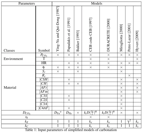
• Approach which is intermediate between the two previous ones. This is the case for the Hyvert [2009] model. Table1 presents the inputs parameters of the simplified concrete carbonation models collected in this work. These parameters are classified into two types: environmental and material parameters. Differences in complexity are observed according to the number of parameters considered in each model.
PCO2 (Pa) is the carbone dioxide pressure on the concrete surface, T (K) is the temperature, HR (%) the concrete
relative humidity,φ the concrete porosity, Sr(%) the saturation degree, Rcthe compressive strength, and[Species] is the
species content into the concrete.
Parameters Models
Classes Symbol Ying-Y
u and Qui-Dong [1987] P apadakis et al. [1991] Bakk er [1993] CEB code CEB [1997] DURA CRETE [2000] Miragliotta [2000] Petre-Lazar [2001] Hyv ert [2009] Environment PCO2 ⇥ ⇥ ⇥ ⇥ ⇥ ⇥ ⇥ ⇥ T ⇥ ⇥ ⇥ HR ⇥ ⇥ ⇥ ⇥ ⇥ ⇥ ⇥ Material φ ⇥ ⇥ ⇥ ⇥ ⇥ ⇥ Sr ⇥ ⇥ ⇥ Rc ⇥ [CSH] ⇥ ⇥ ⇥ [CH] ⇥ ⇥ ⇥ ⇥ [AFt] ⇥ ⇥ [AFm] ⇥ ⇥ [C3S] ⇥ ⇥ [C2S] ⇥ ⇥ [C3A] ⇥ [C4AF] ⇥ ⇥ DCO2 DYu a D Pa ⇥ ktD(t0t)σ ktD(t0t)σ ⇥ ⇥ t0 ⇥ ⇥ kE 1 1 1 ke ke 1 γ2 ke kC 1 1 1 kc kc 1 1 kc
Table 1: Input parameters of simplified models of carbonation
aD
Yu= exp(105.66φ − 0.877)
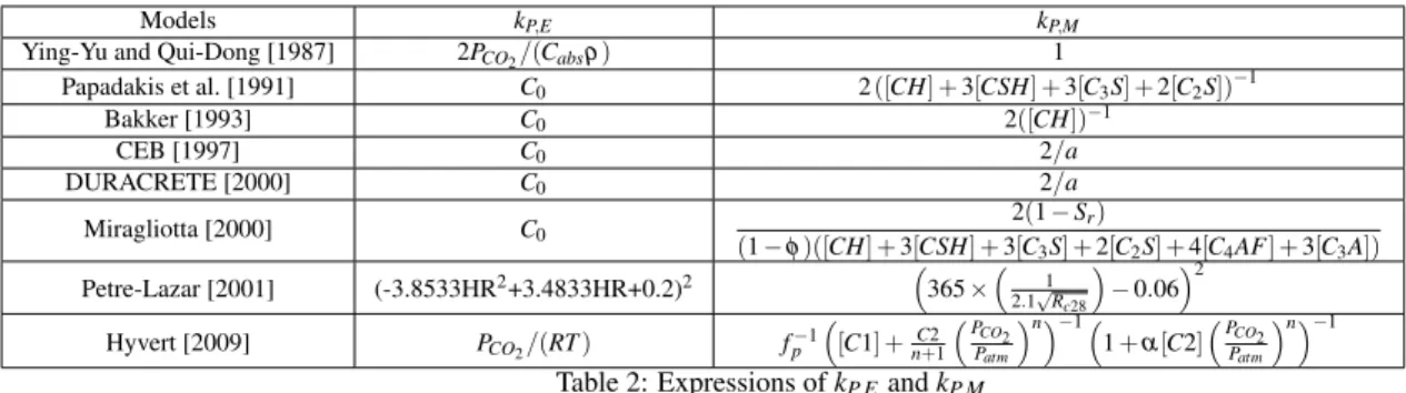
Details about kP,Mand kP,E are given in table 2
3 SENSITIVITY ANALYSIS 3.1 Indicators for sensitivity analysis
For the sake of probabilistic approach, simplified models of carbonation shall be expressed as:
Y= f (t, Z) (3)
Models kP,E kP,M
Ying-Yu and Qui-Dong [1987] 2PCO2/(Cabsρ) 1
Papadakis et al. [1991] C0 2([CH] + 3[CSH] + 3[C3S] + 2[C2S])−1 Bakker [1993] C0 2([CH])−1 CEB [1997] C0 2/a DURACRETE [2000] C0 2/a Miragliotta [2000] C0 2(1 − Sr) (1 − φ)([CH] + 3[CSH] + 3[C3S] + 2[C2S] + 4[C4AF] + 3[C3A]) Petre-Lazar [2001] (-3.8533HR2+3.4833HR+0.2)2 ⇣365⇥⇣ 1 2.1pRc28 ⌘ − 0.06⌘2 Hyvert [2009] PCO2/(RT ) fp−1 ⇣ [C1] + C2 n+1 ⇣P CO2 Patm ⌘n⌘−1⇣ 1+ α[C2]⇣PPCO2 atm ⌘n⌘−1
Table 2: Expressions of kP,Eand kP,M
3.1.1 Elasticity
The elasticity criterion is based on a deterministic approach. It is calculated as follows:
ei=
∆ f (Z,t) ∆zi
(4) where ∆ziand ∆ f(Z,t) are the proportional variations of input ziand model output respectively. An infinite value of ei
means that the model is very sensitive with respect to the variation of the considered parameter, while a value close to zero indicates a low sensitivity. A value of 1 means that a change of zicauses the same variation on yj(case of a linear
model).
3.1.2 Pearson’s correlation coefficient
Pearson’s coefficientρcorestimates the linear correlation between two random variables. It is the ratio of the covariance
between two variables by the product of their standard deviation. In a sensitivity analysis of model parameters, the Pearson’s coefficient is computed between each input parameter and the output. The effect of zion yjat time t is assessed
by the Pearson’s correlation coefficientρcoras follows :
ρcor(t) =
∑(zi− ¯zi)(yj− ¯y)
p∑(zi− ¯zi)2(yj− ¯y)2
(5)
It ranges from -1 to 1. A result close to 1 (in absolute value) indicates a strong correlation between the two parameters while a result approaching zero indicates a low linear correlation. A positive sign means similar trend of variations for both considered variables while a negative one indicates an opposite trend. This indicator is significant in highlighting the physical meaning of the model. This indicator can also be used to rank input parameters according to their influences. However, Pearson’s coefficient is meaningful only if a linear relationship between inputs and output is excepted to exist. 3.1.3 Impact on the output mean value
The previous sensitivity indicators aimed to emphasize the effect of the variability of input parameters upon the model output in terms of proportionality (elasticity coefficient) and statistical dependency (correlation coefficient). The global weight of a parameter can also be estimated by the bias imposed on the output mean value when it remains constant as the other parameters are randomly varying. This is assessed by the bias factor as subsequently explained.
• Firstly, the global mean ¯y of the output is computed: ¯
y(t) ' E( f (t,Z)) (6)
Then, the parameter ziis set at its mean value ¯zi, and the ithcomponent of the input vector Z, now noted Zi0, is no
longer random.
• The bias factor regarding ziis expressed as:
bzi= ¯y(t) − E[ f (t,Zi0)] (7)
3.1.4 Impact on the output’s standard deviation
The standard deviation of the carbonation depth, as well as its coefficient of variation, is an essential information to be acquired in a preventive maintenance or inspection procedure for concrete structures. It is thus of utter importance to examine how the standard deviation of the output model depends on the variability of input parameters. An efficient and simple way is to compute the output standard deviation considering only one random input parameter and setting the others at their mean value. The influence of input zion the output y is evaluated as follows:
σzi/y(t) =
q
3.2 Results for sensitivity analysis
Data with respect to variability of the quantity of hydrates ([CH], [CSH]), unhydrates ([C3S], [C2S], [C4AF], [C3A]),calcium
([C1], [C2]) and cement paste ( fp) are difficult to supply. The variability of these parameters is hence introduced through
the hydration degreeα and the cement content c. The concretes considered in this study are supposed to be exposed to at-mospheric conditions. Thus variability with respect to carbon dioxide content (C0) or pressure (PCO2) are not considered.
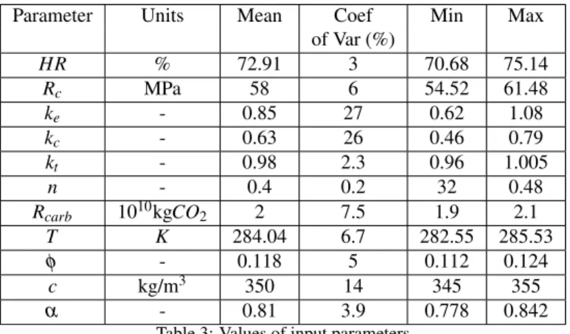
In this paper, results according to one concrete is presented. Ranges of parameter values are reported on table 3. The main objective when fixing range bounds values is to estimate for the considered concrete each input parameter’s range of variation.
Parameter Units Mean Coef Min Max of Var (%) HR % 72.91 3 70.68 75.14 Rc MPa 58 6 54.52 61.48 ke - 0.85 27 0.62 1.08 kc - 0.63 26 0.46 0.79 kt - 0.98 2.3 0.96 1.005 n - 0.4 0.2 32 0.48 Rcarb 1010kgCO2 2 7.5 1.9 2.1 T K 284.04 6.7 282.55 285.53 φ - 0.118 5 0.112 0.124 c kg/m3 350 14 345 355 α - 0.81 3.9 0.778 0.842
Table 3: Values of input parameters
Results for each models are presented in Table 4. Elasticity and Pearson’s coefficient highlighted that the influences remain constant along time. The mean and standard deviations of the response show an evolution of the influences with time, however, the rank of each parameter influence does not change. Therefore only results at 50 years are shown.
Globally, the most influential parameters are those which give informations about the porous media. These are: relative humidity HR which is linked to saturation degree, the cure condition kcand the porosityφ itself. The access of
the carbon dioxide into the concrete bulk depends entirely on these parameters. Therefore, the evolution of carbonation depth is completely dependant on these factors. This explains their prominence. When probabilistic approach is required, considering variability of these parameters seems to be necessary.
The following influential parameters are those which introduce the quantity of species to be carbonated: the cement content c and the hydration degreeα. When c and α are important, at each units of depth, the quantity of species to be carbonated is important. Consequently, kinetic of the carbonation depth evolution is slow. This implies that values of elasticity and Pearson’s coefficient are negative. With respect to updating proceduresα appears to be relevant. Indeed, in addition to its quite important influence, this parameter increases with time. Despite the fair importance of c (as forα), this parameter could be considered as constant. It is theoretically constant and describing variability with respect to this parameter in a real structure is difficult.
Elasticity is an indicator of local sensitivity analysis. The selected disturbance on any input is a 10 % deviation from the mean value. This could not be realistic for some parameters and hence causes bias on results. Generating the variability into realistic intervals is therefore necessary. It has been observed that the influence of each parameters remain constant along time with respect to elasticity.
The Pearson’s correlation coefficient is fruitful to rank input parameters according to their influences. It also allows the distinction between inputs whose increase produces decrease of the output and those which produce the opposite effect. However, this coefficient is meaningful when a linear relationship exists between the input and output. The influences of each parameter do not change with time.
Computing the deviation from global average of the response allows to estimate the attributable variability to each input parameter. The values are generally low for all models. It can be noticed that the values of influences change with time. However the rank of each parameter according to the importance of its influence does not change.
Finally, the standard deviation of the response provides informations on the effect of the variability of a given input on the variability of the output. The main tendencies of the models with respect to input parameters are described. Although evolution with time of influences is observed, the rank of each parameter according to the importance of influence remains. 4 GAUSSIAN RANDOM FIELD
A scalar random field H(x, ω) is a collection of random variable indexed of a continuous parameter x2 B, when B is an open set of Rddescribing the geometry of the physical system (generally d=1, 2, 3). For a given x02 B, H(x0, ω) is a
random variable, and for a given outcomeω02 ω, H(x,ω0) is a realization of the field.
This work focusses on Gaussian random fields, whose realizations are generated thanks to the Karhunen-Loeve ex-pansion: H(x, ω) = µH+ σH n
∑
1 p λiξifi(x) (9)Models Param E P M Std DuraCrete Rcarb -0.47 -0.12 1 3.27 ke 0.49 0.37 1.02 11.84 kc 0.49 0.35 1.02 11.37 kt 0.49 0.04 1 1 n -1.45 -0.85 1.13 27.56 CEB Rcarb -0.47 -0.05 -0.09 1 ke 0.49 0.25 1 5.44 kc 0.49 0.24 0.95 5.22 n -2.29 -0.93 -13.50 21.47 Oxand HR -1.77 -0.44 1 1 fc28 -11.52 -0.88 -0.28 2.07 Ying-Yu HR -2.92 -0.68 -0.08 8.08 α -0.53 -0.15 0.01 1.78 Sr 1.09 0.71 -3.038 8.41 φ 0.89 -0.16 1 4.13 c -0.77 -0.09 -0.01 1 Mv -0.91 -0.16 -0.37 6.27 Miragliotta HR -2.92 -0.55 -0.10 20.73 α -0.12 -0.05 -0.01 1 Sr -0.98 -0.58 1 31.45 φ 2.06 0.61 -0.38 22.78 c -1.2 -0.12 -0.06 4.20 Papadakis HR -2.92 -0.79 -2.97 19.01 α -0.12 -0.04 -0.07 1 c -1.17 -0.17 -1.17 3.77 φ 1.39 0.62 1 14.67 Hyvert HR -4.3 -0.7 -0.26 53.30 T -0.47 -0.1 -0.003 1 kc 0.49 0.66 1 49.73 φ 0.68 0.17 0.11 13.55 c -1.3 -0.1 -0.03 7.75 α -1.2 -0.2 -0.14 15.99
Param = parameter, E = Elasticity, P = Pearson’s coefficient, M = deviation from global mean⇥106, Std = Standard deviation of output⇥104
whereµH is the mean value of the stochastic field H, σH is the standard deviation of H, n is the retained number of
terms in the truncated expansion,ξiis a set of centred reduced Gaussian random variables,λiand fiare respectively the
eigenvalues and eigenfunctions of the covariance functionρ(∆x). This function describes the spatial correlation structure of the random field. The following exponential form for this function is considered:
ρ(∆x) = exp ✓ −∆x b ◆ (10)
where ∆x is the distance and b> 0 is a dimensional parameter.
In this work, the construction of ρ(∆x) is made by meshing the geometry of the studied system. Regarding the estimation of b, two major procedures have been reported in the literature. First, the procedure reported by Li [2004], the Maximum Likelihood Estimation method (MLE) is used, in which different values for the model parameter of the proposed ACF (Auto Correlation Function) model is assumed and the value that maximizes the corresponding MLE is taken as the model parameter. In the second procedure, proposed by Vanmarcke [1983], a proposed ACF model (here exponential form) can be adjusted to provide the best fit to the actual sample correlation coefficients thereby providing estimation of the corresponding model parameter. In this work, b will be identified through bayesian network, therefore a range of values is needed which minimum and maximum bounds are respectively: the distance between the two closest points, and the length of the structure.
5 UPDATING PROCESS THROUGH BAYESIAN NETWORK
The physical parameter which spatial variability is analysed is carbonation depth. Measured data of carbonation depth are supposed to be available on some limited numbers of points on a concrete structure surface through inspection with destructive or non destructive test. Carbonation depths are also predicted by physical models reported on section 2 (predicted data) and at the same points where measured data are available. These predictions are used for the learning process of the bayesian network. It is to be remembered that a bayesian network is a probabilistic graphical model that involves a set of random variables which are interconnected to one another by conditional dependencies.
5.1 Learning process
The parents nodes are: the mean valueµHand the standard deviationσHof the field, and the parameter b. The mean
range bounds are the minimum and the maximum of mean values at each points of measurement. So is it for the standard deviation. As it was previously mentioned, the bounds of the b values are the distance between the two closest points, and the length of the structure.
Children nodes are the values generated at each point of measurement/prediction. 100 triplets(µH, σH, b) are
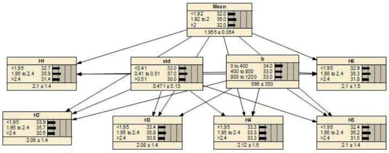
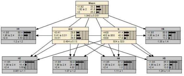
ran-domly generated using latin hypercube sampling from their respective ranges. For each triplet, 100 values are generated using Karhunen Loeve expansion at each point. Therefore at each point, 10000 values are available and the distribution histogram is established. Using Netica of the Norsys software Corp, the conditional probabilistic tables are computed automatically. Figure 1 presents an example with 6 points of measurement/prediction (H1 to H6).
5.2 Validation process
In real case, with some limited measurements, the random field parameters are identified through the network. In order to check the compliance of the network, a validation process was achieved. With a given triplet of parent nodes, 100 values at each point of measurement were generated. Those values are entered at each corresponding children nodes. Then, the parent nodes are identified. If the right triplet is identified, it can be concluded that the network is valid for the considered case.
Numerous cases have been tested. Figure 2 and 3 represent examples of results, using the triplet t1(1.95, 0.6, 600) and
t2(2, 0.41, 300) respectively. t1gives values near of the middle of each considered state while t2presents values close to
states bounds.
With respect to t1, mean and standard deviation are identified at more or less 40% of probability (39.6 and 41.6 for
mean and standard deviation respectively). So is it for b (40.8 %). However, for this latter, it is less than the probability of one wrong state (¡400). This could be explained that this wrong state has already presented the highest probability during the learning process (see figure 1). Therefore, it could be assumed that the identification is successful.
Regarding to t2, identification seems to be more tricky. With respect to the mean value, 2 is exactly a boundary state.
Therefore, the identification should give equivalent probabilities on both 2 sides of the boundary. However, given that the state 1.92 to 2 has presented higher probability (36%) during the learning process (figure 1), the identification tends to this state. So is it for the standard deviation which is on the boundary state (0.41). Privilege is given to the state (0.41 to 0.51). Only b is clearly identified (48.9%) which is relatively far from boundary state (300).
Figure 2: Validation test for the triplet t1
6 COMMENTARY AND CONCLUSIONS
Sensitivity analysis has been carried out in order to visualise these models ability to transfer uncertainties. Moreover hand, it allows to quantify the relative importance of each input parameter. Within the project framework, input parameters are preferably supplied through non destructive tests. Therefore, models for which prominent input parameters could be assessed with that test method, would be privileged.
The following indicators are used for the sensitivity analysis: elasticity, Pearson’s linear correlation coefficient, impact on the mean and standard deviation of the response.
The use of several indicators enriched the sensitivity analysis. Indeed, all indicators do not provide the same level of information, thus main tendencies are quite well described.
The parameters which describe the porous media appear to be the most influential ones. These are HR which is linked to saturation degree, kcwhich gives an assessment of the quality of the firsts centimetres from the exposed surface, and the
porosityφ . The access of carbon dioxide depends entirely on these parameters. When probabilistic approach is needed, considering the variability of these parameters seems to be necessary.
The next important parameters are those which introduce the quantity that can be carbonated: the hydration degreeα and the cement content c.
The next step of the project is to analyse the ability of the simplified model to take into account spatial variability. Indeed, maintenance strategy against corrosion are to be applied to a structure surface. The analysis is supposed to be led in two steps:
• updating through bayesian network the spatial variability parameters of carbonation depth predication by mod-els, with measured data. It has been shown within this study that this process provides relatively correct results.
Figure 3: Validation test for the triplet t2
However, other cases are be tested to enrich the result.
• through models inversion, the input parameters are determined and their spatial variability will be described. The results will be compared to spatial variability of measurements of these input parameters. Deviations will be anal-ysed thereby new comparison of models could be achieved. This step is not yet completed. As it is shown in section 2, simplified models of carbonation are time dependant. Therefore, for a correct inversion, the number of dates at which data are available should be at least equal to the number of input parameters of the studied model.
These processes are conceived in order to advise the building manager for the choice of the appropriate model with respect to his needs, his constraints and available data.
7 ACKNOWLEDGEMENTS
This study has been carried out in the framework of the research project EvaDeOS (French National Research Agency - ANR 2011-VILD-002-01)
REFERENCES
R. Bakker. Model to calculate the rate of carbonation in concrete under different climatic conditions. Technical report, CMIJ bv Laboratorium, Imuiden,, The Netherlands, 1993.
CEB. New approach to durability design: an example for a carbonation induced corrosion. Bulletin 238, CEB, 1997. DURACRETE. Duracrete - final technical report - general guidelines for durability design and redesign. Technical Report
BE95-1347/R9, The European Union - Brite Euram III, 2000.
N. Hyvert. Application de l’approche probabiliste de la durabilite des produits prefabriques en beton. These de genie civil, Universite de Toulouse III-Paul Sabatier, 2009.
Y. Li. Effect of spatial variability on maintenance and repair decisions for concrete structures. PhD thesis, Delft Univer-sity, Delft, Netherlands., 2004.
R. Miragliotta. Modelisation des processus physico-chimiques de la carbonatation des betons prefabriques - Prise en comptes des effets de paroi. PhD thesis, Universite de la Rochelle, 2000.
V.G. Papadakis, C.G. Vayenas, and M.N. Fardis. Fundamental modelling and experimental investigation of concrete carbonation. ACI Materials Journal, 4(88):363–373, 1991.
I. Petre-Lazar. Evaluation du comportement en service des ouvrages en beton arme soumis a la corrosion des aciers. Phd civil engineering, Universite Laval, Quebec, 2001.
E. Vanmarcke. Random fields: analysis and synthesis. Technical report, MIT Press, Cambridge, Mass; London., 1983. L. Ying-Yu and W. Qui-Dong. The mechanism of carbonation of mortars and the dependence of carbonation on pore
RESPONSIBILITY NOTICE