New methods for the multi-skills project scheduling problem

(1)

HAL Id: tel-00789769

https://tel.archives-ouvertes.fr/tel-00789769

Submitted on 18 Feb 2013

HAL is a multi-disciplinary open access

archive for the deposit and dissemination of sci-entific research documents, whether they are pub-lished or not. The documents may come from teaching and research institutions in France or abroad, or from public or private research centers.

L’archive ouverte pluridisciplinaire HAL, est destinée au dépôt et à la diffusion de documents scientifiques de niveau recherche, publiés ou non, émanant des établissements d’enseignement et de recherche français ou étrangers, des laboratoires publics ou privés.

New methods for the multi-skills project scheduling

problem

Carlos Eduardo Montoya Casas

To cite this version:

Carlos Eduardo Montoya Casas. New methods for the multi-skills project scheduling problem. Au-tomatic Control Engineering. Ecole des Mines de Nantes, 2012. English. �NNT : 2012EMNA0077�. �tel-00789769�

(2)

Thèse de Doctorat

Carlos Montoya

Mémoire présenté en vue de l’obtention du

grade de Docteur de l’École des mines de Nantes

sous le label de l’Université de Nantes Angers Le Mans

Discipline : Informatique

Spécialité : Recherche Opérationnelle Laboratoire : IRCCyN

Soutenue le 13 decembre 2012 École doctorale : 503 (STIM) Thèse n° : 2012 EMNA 0077

New methods for the Multi-Skill Project

Scheduling Problem

JURY

Rapporteurs : M. Christian ARTIGUES, Directeur de Recherche, LAAS, CNRS, Toulouse

M. Jacques CARLIER, Professeur, Université de Technologie de Compiègne Examinateurs : M. Pierre DEJAX, Professeur, Ecole des Mines de Nantes

M. Boris DETIENNE, Maître de Conférences, Université d’Avignon

M. Emmanuel NÉRON, Professeur, Université François-Rabelais de Tours Directrice de thèse : MmeChristelle JUSSIEN-GUÉRET, Professeur, Université de Angers

(3)

(4)

Acknowledgements

I would like to express my thanks to all the people who have been very helpful to me during the whole phD experience. I have to outline also that the work done during my phD took place in the Ecole des Mines Nantes and the IRCCyN.

In the first place I would like to thank Christelle Jussien-Guéret who was the first person to consider me as a potential phD student. Thereafter, thanks to that initial support I was able to start this amazing journey, in which I had the opportunity to experience a new life experience in a different country and culture.

I would like also to thank my supervisors Odile Bellenguez-Morineau and David Rivreau for their valuable suggestions, feedback, patience, guidance and support all along this last three years. I would like to thank as well Eric Pinson, for his valuable help and contri-bution in the work done during my phD. Thanks is owed also to the project LigéRO for funding my phD thesis.

Subsequently, I want to thank Christian Artigues and Jacques Carlier for accepting to be the reviewers of my thesis and therefore for their remarks and suggestions allowing me to enforce certain perspectives that could lead to interesting findings in my research subject.

I want to thank as well Emmanuel Néron, Boris Detienne and Pierre Dejax for partici-pating as members of the jury of my thesis and for their feedback and perspectives on the work done during my phD.

Finally I would like to thank all the good friends that I have the opportunity to met and cross by during this last three years, allowing me to have a lot of nice experiences and memories that I will always keep and treasure.

(5)

(6)

List of Tables

2.1 Required skills description . . . 6

2.2 Number of workers required per activity (bi,k) per skill . . . 7

2.3 List of skills mastered per worker (M Sm,k) . . . 7

2.4 Average number of variables and constraints for each ILP . . . 23

2.5 Makespan performance of each ILP . . . 24

2.6 Linear relaxation performance of each ILP . . . 24

2.7 Global performance of each ILP . . . 24

3.1 Linear relaxations comparison between CG1and the time indexed models 53 3.2 Comparison between CG approaches proposed . . . 54

4.1 Branching strategies performance . . . 66

4.2 Performance comparison between the proposed B&P approaches . . . 66

4.3 Performance comparison between the proposed B&P approaches for in-stances solve to optimality . . . 67

4.4 B&PTW computational time performance measures . . . 67

4.5 Performance strategies for pruning nodes . . . 68

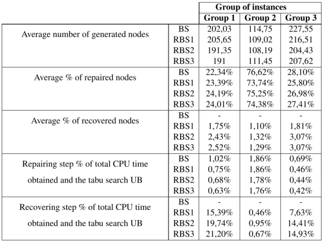
4.6 Performance comparison between the proposed beam search approaches . 81 4.7 Repairing and recovering steps performance comparison between the pro-posed beam search approaches . . . 83

4.8 Impact of the weight definition criteria and the total completion time con-straint in the recovering beam search ILP . . . 84

5.1 Summary of the obtained lower bounds results . . . 103

5.2 Summary obtained results of the two-phase solution approach . . . 103

5.3 Performance measures of the two-phase solution approach . . . 104

5.4 Summary obtained results . . . 105

7.1 Liste des compétences . . . 121

7.2 Besoins des activités . . . 122

7.3 Compétences maitrisées par chaque personne (M Sm,k) . . . 122

7.4 Comparaison entre TIMWS, CG et CGLR . . . 132

7.5 Comparaison de performance entre B&PTW et B&PCB . . . 137

7.6 Comparaison de performance entre B&PTW et B&PCB pour les instances pour lesquelles la solution optimale a été obtenue . . . 138

7.7 Comparaison des performances entre BS et RBS . . . 142

(11)

(12)

List of Figures

2.1 Precedence relations Graph G . . . 7

2.2 Gantt chart of an optimal solution . . . 8

3.1 Precedence relations Graph G . . . 32

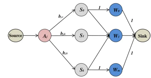
3.2 Graph Fcskills assignment for activity Ai. . . 38

4.1 Example of the dichotomic time-windows branching strategy. . . 58

4.2 Graph Fa skills assignment for the candidate activity Aj without consid-ering an assignment cost for each worker. . . 60

4.3 Representation of the Recovering Beam Search. . . 72

5.1 Two-phase approach for solving the MSPSP. . . 90

5.2 Processing among time of activities A6, A7and A8 . . . 94

5.3 Workers assignment for each activity Ai. . . 95

5.4 Processing of activities in I . . . 97

5.5 Procedure for identifying subset I . . . 98

5.6 Processing among time of activities in I . . . 99

5.7 Procedure for generating an overlapping subsets cut . . . 101

7.1 Graphe G . . . 122

7.2 Exemple d’une solution optimale . . . 123

7.3 Graphe Fc: Affectation des compétences pour l’activité Ai. . . 131

7.4 Example of the dichotomic time-windows branching strategy. . . 134

7.5 Graph Fa skills assignment for the candidate activity Aj without consid-ering an assignment cost for each worker. . . 135

7.6 Approche en deux phases pour résoudre le MSPSP. . . 144

7.7 Procédure pour identifier le sous-ensemble I . . . 148

(13)

(14)

1

Introduction

Resource management plays an important role for enhancing the competitiveness of a company. Particularly, the correct management of human resources represents an impor-tant issue for organizations. Furthermore, defining the schedule and assignment of tasks among the available resources are important duties that take place in a normal daily basis in any organization. In the most of planning and scheduling tasks the hardest constraints are caused by restricted resources. This is why resource allocation is an important com-ponent of many real-life planning and scheduling tasks. From algorithmic point of view it can be considered either as a part of the planning or a part of the scheduling. A mixed ap-proach is also used. Thereby, the methods used to perform such duties must be oriented in giving a good use to resources considering their capacity, cost and availability. There are several scheduling environments that deal with the aspects previously mentioned, thus, in this thesis we focus in a particular one, which involves the management of scarce re-sources in a Project Scheduling environment. Moreover, these issues are addressed by the Resource Constrained Project Scheduling Problem (RCPSP) [22] which is a classical scheduling problem that received major attention in the last years.

The RCPSP deals with a given number of activities that have to be scheduled on a set of resources. It also takes into account precedence relation between activities and limited resource availability. The interest in extending the practical applications of the RCPSP encouraged researchers to work on different extensions that capture several variants and features related to specific real life situations [22, 83, 93, 2, 64]. Different optimization criteria have been addressed for the RCPSP, from which minimization of the makespan is among the most popular ones. Although, other time-based objectives based on lateness, tardiness, and earliness present a particular importance as well. Additionally, there are other objectives based on costs assignment related to resources and/or activities and/or time. Also, the concept of cash flow has been taken into account for maximizing the net present value of a project [22].

(15)

In this context, it is important to notice that scheduling the activities of a project is partially conditioned by the constraints and specifications of the available resources. Sub-sequently, we can define such constraints and specifications by identifying the different types of resources that are normally considered [64] in a project:

– Renewable resources: Such a type of resources can be used whenever they are available in each period with its full capacity.(e.g staff members, machines and equipment). – Non-renewable resources: This type of resources is available only in a given amount

for the entire project duration (such as money). A good example would be a predefined budget for the project.

– Doubly constrained resources: They are limited both for each period and for the whole project. Money, can be an example if both the budget and the per-period cash flow of the project are limited.

– Partially renewable resources: They allow to define capacity limitations over arbitrary subsets of periods. This type of resources permits for example to represent workers for which their working hours are limited by the contract duration.

Furthermore, when dealing with human resources, we can also identify that particularly in service firms like health care enterprises, call centers and also in different manufacturing environments the utilization of staff members with multiple skills is commonly required. Thus, in order to consider such a feature, we also have to distinguish the resources that are able to fulfill a unique kind of requirement (mono-skilled) from the ones that are capable to satisfy several ones (multi-skilled) [65]. This concept can also be extended to a scheduling environment in which the resources are multi-purpose machines, that can be able to perform several types of tasks [23].

Thereafter, given its practical importance, the notion of skills has been addressed by several authors. More precisely, in the field of personnel scheduling and assignment there are several problems that deal with multi-skilled resources [45]. In this thesis we aim at considering the assignment of several resources with different skills to the same task (activity) under a Project Scheduling environment. More precisely, besides using multi-skilled resources, we consider that a given activity might have several skill requirements.

Furthermore, we focus on one particular extension of the RCPSP, which is known as the Multi-Skill Project Scheduling Problem (MSPSP). This problem was originally proposed by Néron and Baptista [93]. It mixes both the classical RCPSP and the Multi-Purpose Machine model. The aim is to find a schedule that minimizes the makespan. Practical applications can be related to call centers, construction of buildings, production and soft-ware development planning. A specific example of a real life application, with similar features to the MSPSP can be found in the work of Cordeau et al. [31]. They proposed a solution method for the technician and task scheduling problem arising in a large telecom-munications company. Valls et al. [112] deal also with a real-life problem that comes up in the daily management of service centers.

(16)

In this work, we intend to propose several methods for solving the MSPSP. We give a particular importance to exact methods with the purpose of obtaining optimal solutions for small and medium sized instances. Best results obtained so far were achieved by Bellenguez-Morineau and Néron [17] by means of a heuristic approach. In addition, these last mentioned authors also founded strong lower bounds for the different available instances, obtaining that there are still several small and medium sized instances for which optimality is still to be proven.

This thesis is organized as follows: Chapter 2 presents the detailed description of the Multi-Skill Project Scheduling Problem, followed by an example based on a real life application. Afterwards, we propose a review of related problems for identifying and understanding differences and similarities. Thereafter, we introduce the previous work done on the MSPSP and other approaches for problems with similar features to the ones treated in this thesis. Hence, we explain and introduce all the instances that are used as benchmark for the MSPSP. More precisely, we introduce five different integer linear programming (ILP) models, which help us to represent the MSPSP from different per-spectives. Thereby, we discuss their efficiency and limits, based on several computational experiments carried out on instances taken from the literature.

Subsequently, in chapter 3 we proposed different procedures for obtaining makespan lower bounds based on a Column Generation (CG) approach. Hence, we introduce several mathematical formulations and different resolution techniques. Thereby, we present the respective results, and then, we compare the obtained makespan lower bounds with the linear relaxations values of the ILP models.

Thereby, in chapter 4 we introduce both, exact and heuristic approaches for solving the MSPSP, based on the utilization of the Column Generation (CG). Therefore, initially, with the purpose of obtaining an integer optimal solution, we developed a Branch-and-Price (B&P) procedure. Subsequently, we describe the different branching and node filtering techniques, along with the methods we used for getting a makespan upper bound. There-after, we present the respective results and conclusions. Furthermore, with the purpose of solving big size instances, we introduce a recovering beam search (RBS) approach that exploits the structure of the branch and price procedures discussed in a previous section and integrates the resolution of different mathematical models. Hence, we introduce and analyze the obtained results.

Finally, in chapter 5 we explore a two-phase procedure, in which new constraints (cuts) are generated iteratively until ensuring an optimal schedule. The first phase involves the definition of the starting times of the activities of the project. Subsequently, in the second phase we focus on finding a feasible assignment of workers that allows the execution of the activities according to the starting times defined in the first phase. Thereby, we present and analyze the obtained results.

(17)

(18)

2

Problem definition and formulation

This chapter presents the detailed description of the Multi-Skill Project Scheduling Prob-lem (MSPSP). All the related notations and specifications of the probProb-lem are explained, then, we present an example based on a real life application. We also describe the features of the expected solution after doing the schedule of the project presented in the example. Afterwards, we introduce the literature review of related problems in order to identify and understand differences and similarities. Thereby, we introduce the previous work done on the MSPSP and other approaches for solving problems that deal with the scheduling and assignment of multi-skilled resources.

2.1 Problem presentation

The Multi-Skill Project Scheduling Problem (MSPSP) is a known project scheduling problem, which is mainly composed by three elements: Activities, resources and skills. These elements are detailled below:

Activities

A project is composed by a set of activities A = {A0, . . . , AN}. Within this set, we

also define two dummy activities A0 and AN to represent respectively the beginning and

termination of the project. Activities are submitted to precedence relations, which implies that certain activities have to be finished before others can start [64]. Thus, each activity Ai has a corresponding set of successors Ei+ and predecessors E

−

i . This is handled by

depicting the project as a directed graph (G) where an activity is represented by a node and the precedence relation between two activities is represented by a directed arc (Ai, Aj)

where Aj ∈ Ei+ [83]. This arc also represents the minimal duration time between the

starting time of Ai and the beginning of any of its direct successors. Thereafter, such a

(19)

All the activities must be scheduled in order that the total duration time of the project (makespan) is minimized. Given that the starting time of an activity Ai is denoted by ti,

its completion time will be given by ti+ pi, since preemption is not allowed.

Resources and skills

In a classical MSPSP context, the resources we focus on for performing all the activities of a project are staff members. Thus, we can ensure that we deal only with a renewable type of resources. Due to the nature of the treated problem, we consider a set W of M workers and a set S of K skills. Each single resource Wm (Wm ∈ W ) is able to carry

out a given subset of skills. The distribution of skills in the workforce is denoted by a parameter M Sm,k which takes the value of one if worker Wm masters skill Sk, or zero

otherwise.

Furthermore, a given number of workers must be assigned to each one of the required skills to perform a given activity. This implies that a single activity might need the uti-lization of several skills. The constraints linked to the notion of skills are described as follows [93]:

– A total number of bi,k workers that master each skill Skmust be assigned to activity Ai.

If Skis not required by Ai, we set bi,k = 0.

– A worker Wmcan be assigned only for using a skill he masters, i.e M Sm,k = 1.

– A worker Wmcan only use one skill on one activity at a given time t.

– All the workers assigned to a specific activity Ai must work simultaneously during its

whole processing time ([ti, ti+ pi[).

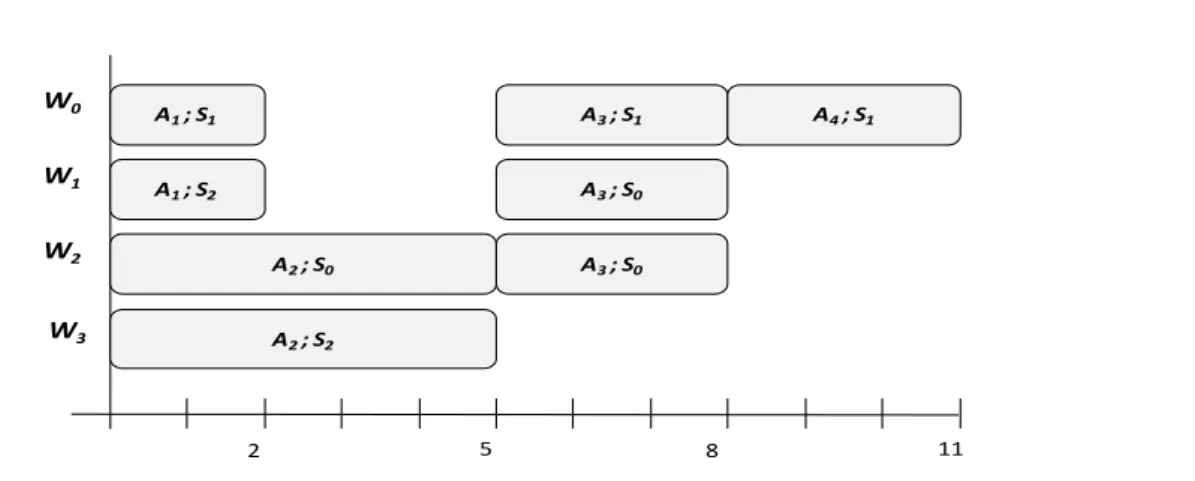
Thereby, we present all the features described above with an example, which is based on a real life application for the development of software products. Here we consider a small project of three activities, four workers and three skills. Table 2.1 shows the description of each skill. Table 2.2 gives the skills requirement of each activity. Table 2.3 shows the description of the staff members in terms of the skills. Figure 2.1 presents the graph of the project with the processing times of the activities. Figure 2.2 shows a Gantt chart of a feasible solution that fulfills all the constraints.

S0 Programmer

S1 Data Base Designer

S2 Webmaster

Table 2.1: Required skills description

From this table it can be noticed that W0 masters S1 and S2, while W2only masters S0.

This table shows for instance that A3 requires two workers that masters S0 and one

(20)

S0 S1 S2

A1 - 1 1

A2 1 - 1

A3 2 1

-A4 - 1

-Table 2.2: Number of workers required per activity (bi,k) per skill

S0 S1 S2

W0 - 1 1

W1 1 - 1

W2 1 -

-W3 1 - 1

Table 2.3: List of skills mastered per worker (M Sm,k)

From this table we can see that W0 masters S1and S2, while W2only masters S0.

A0 A1 A2 A3 A4 A5 0 0 5 2 3 3 Ai Aj pi

Figure 2.1: Precedence relations Graph G

Notice that A0 and A5are additional dummy activities which represent the beginning and

termination of the project respectively. Arcs weight represents the processing times of each activity.

It is important to notice from figure 2.2, that once A1 and A2 are scheduled at time

zero, A3 cannot start at time two, due to the fact that at that moment there are not enough

available workers that masters S0 to fulfill all the requirements of such an activity. In

addition, the fact that A3 is scheduled at time five implies that W0, who is the only one

that masters S1, will not be available until time eight. Thus A4 can start only until that

moment.

Finally, according to the known fact that the RCPSP is already an N P-Hard optimiza-tion problem, thus the MSPSP is also N P-Hard in the strong sense [2]. Thereby, these two problems are equivalent if each worker master only one skill.

(21)

W0 W1 W2 W3 A1 ; S1 A1 ; S2 A2 ; S0 A2 ; S2 A3 ; S1 A3 ; S0 A3 ; S0 A4 ; S1 5 8 11 2

Figure 2.2: Gantt chart of an optimal solution

2.2

2.3 Job Shop Scheduling Problem

The Resource constrained Project Scheduling Problems are considered as a generalization of the JSSP, thus we start by giving an overview of its most important features. The Job Shop Scheduling Problem (JSSP) is a well-known disjunctive scheduling problem which can be described as follows:

– The problem consists of a set J of n jobs and set M of m machines. – Each job j ∈ J must be processed exactly once on each machine.

– Each job defines an order in which it should be processed on the machines. For a job j ∈ J let j(k), πj(k)1 ≤ k ≤ m, denote the kth machine for j.

– The processing of job j ∈ J on machine πj(k) is called an operation, and denoted oj,k.

An operation oj,k has an duration of pj,k and cannot be preempted, i.e., the processing

of an operation cannot be interrupted and then resumed at a later point in time. – Each operation of a job must occur one after the other.

– Only one operation may be in progress at a time on each machine.

– The objective is to minimize the project makespan, i.e., the total time needed to com-plete all operations.

– The JSSP is N P-Hard for |M | ≥ 2 and |J | ≥ 3 (see Garey et al. [54]).

The JSSP is from a modeling point of view very simple, yet general enough to model many real-life situations, such as a factory floor, where there is no choice of which ma-chine to be used for a given operation, and each mama-chine can only perform a single oper-ation at a time.

(22)

It is important to mention that there are other extensions of the JSSP that share some similarities with Resource constrained Project Scheduling Problems. Particularly, we out-line the FJSSP, which deals with the assignment of several machines that can be assigned to the same operation (mono-skilled resources). More precisely, another extension of the JSSP suitable with some of the features of the MSPSP is the Multiprocessor Job Shop Scheduling [75], which considers that each operation may require the utilization of sev-eral resources simultaneously.

2.4 The Cumulative Scheduling Problem

Another scheduling problem encountered in the literature is the Cumulative Scheduling Problem (CuSP) which is N P-Hard ([6]). This problem introduces the concept of cu-mulative resources, which is an important resource feature considered in the Resource Constrained Project Scheduling Problems. The CuSP can be described as follows:

– A set A of activities must be performed on a single resource which has a constant capacity R.

– Each activity Ai ∈ A has a processing time pi (non-preemptive), and requires bi units

of the resource while it is in progress.

– Each activity Ai ∈ A, is associated with a release time tri and due date tdi, and the

activity must be performed in the interval [tr

i, tdi]. Let T be a set of time steps.

– Usually, the aim is to find a feasible schedule, which minimizes the makespan.

The notion of cumulative resources plays an important role in Resource Constrained Project Scheduling Problems. It allows us to identify different features of the resources used in a given Project Scheduling environment.

2.5 Resource Constrained Project Scheduling Problem

As we discussed before, the MSPSP is considered as an extension of the RCPSP. Hence, we give a little overview of the main features of such a problem [22]. For keeping the similarity with the MSPSP, next description only considers renewable resources. Never-theless, notice that there are other types of resource that can be considered such as: non-renewable resources, doubly constrained resources and partially non-renewable resources.

A project consists of a set of activities A = {A0, . . . , AN} and a set R of resources,

where activities A0and AN are dummy activities representing the start and completion

of the project, respectively. Each activity Ai has a processing time of pi, and during

its non-preemptive processing it requires bi,k units of resource Rk ∈ R. Each resource

Rk ∈ R, has capacity Bk in each time period. Activities must follow a precedence

relation, which implies that certain activities have to be finished before others can start [64]. Thus, each activity Aihas a corresponding set of successors Ei+.

(23)

Due to the N P-Hardness of these project scheduling problem exact methods fail on large instances [2], but there are many constructive heuristics and local search techniques avail-able to find good quality solutions. For an overview of these solution approaches the reader is referred to [83].

An importance thing to notice, is that despites that the scheduling of the RCPSP is entirely defined by the starting times of the activities, for the MSPSP it is mandatory to determine the assignment of workers according to their skills.

2.6 Multi-Mode Resource Constrained Project

Schedul-ing Problem

Another interesting generalization of the RCPSP is the Multi-Mode Resource Constrained Project Scheduling Problem, which is also an N P-Hard problem. Thereafter, we define it as follows [22]:

– – – –

– A project consists of a set of activities A = {A0, . . . , AN} and a set R of resources,

where activities A0and AN are dummy activities representing the start and completion

of the project, respectively.

– Each activity Ai can be performed in a number of different modes Mi = 1, ..., |M j|,

each representing an alternative way of performing the activity. – Each resource Rk∈ R, has capacity Bkin each time period.

– When an activity Ai is scheduled in mode m ∈ Mi, it has a processing time of pi,m

(non-preemptive) and requires bi,k,munits of resource Rk ∈ R in each time period.

– Activities must follow a precedence relation, which implies that certain activities have to be finished before others can start [64]. Thus, each activity Ai has a corresponding

set of successors E_i+.

For keeping similarity with the features of our studied problem, in the previous description we considered only renewable resources. There are several approaches that have been used for solving this problem, thus the reader is referred to [64].

The MSPSP can be seen as a Multi-Mode RCPSP [2]. In the context our problem, the Multi-Mode approach would require representing all the feasible combinations of workers to execute an activity [93].

For illustrate the previous statement, let us remember the described example for the MSPSP (see section 2.1).If we want to define the modes of execution of A2, we would

have to consider seven modes to perform such an activity, given by the next combina-tion of workers: (W0, W1); (W0, W2); (W0, W3); (W1, W2); (W1, W3); (W2, W3). Each

combination could represent more than one mode according to how skills are distributed among the respective couple of workers. For example in the combination (W1, W3) both

(24)

this case there are two modes of skills assignment between both workers: (i) W1 uses S0

and W3 uses S2or (ii) W1uses S2 and W3 uses S0. In such situation, both modes implies

that during the execution of A2 the two workers will not be available.

If we consider bigger projects the number of modes could be really huge, making im-possible to implement the existing methods related to the resolution of the Multi-mode RCPSP [2].

2.7 Multi-purpose machine model

Now, for including the notion of multi-skilled resources in the RCPSP, we introduce The Multi-purpose machine model [23], which also has a N P-Hard complexity.

The general features of this problem are described as follows: – There are m different machines, distinguish from M1 to Mm.

– There are N jobs that must be scheduled.

– Each job j must be executed by a machine selected from a subset of machines that are able to carry it out during a constant processing time pj.

– Each machine is able to perform a subset of jobs.

This problem allows us to put in context the notion of resources that are able to perform different operations (multi-skilled) as it occurs with the MSPSP.

The Multi-purpose machine model differs from the MSPSP in the fact that jobs have an unitary requirement, thus the related solution methods cannot be directly applied for solv-ing the MSPSP, considersolv-ing that in our problem we have to deal with the synchronization of certain resources for executing a single activity.

2.8 Multi-skilled personnel assignment background

After introducing different problems with similar features to the ones of the MSPSP, we established the importance of multi-skilled resources for determining the difference with other RCPSP problems. Thus, we aim on identifying how the notion of skills have been considered in personnel scheduling and assignment problems that deal particularly with multi-skilled resources.

Different papers related to scheduling and personnel assignment considers the notion of skills. On one hand, we have several problems that deal with multi-skilled resources, but only one resource can be assigned to a task. For example, the Home Health Care problem (HHC) considers the utilization of nurses with several qualifications or skills that has to be assigned into a set of jobs. Usually in this type of problem a single nurse is assigned to a job, but such nurse must have the set of skills required for the job. Related to this matter, Begur et al. [13] proposed a spatial decision support system for scheduling and routing

(25)

home-health-care nurses, while Bertels and Fahle [18] proposed a combination of linear programming, constraint programming, and meta-heuristics. Another interesting problem with similar features is the Skilled Workforce Project Scheduling Problem (SWPSP), for which Valls et al. [112] proposed a hybrid genetic algorithm that combines local searches with genetic population management techniques to solve it.

On the other hand, some problems consider the assignment of several workers with different skills to the same task. For instance, Eveborn et al. [47] worked on an extension to the HHC problem and proposed a set partitioning model, and as a solution method they developed a repeated matching algorithm. More recently, Cordeau et al. [31] de-veloped a construction heuristic and an adaptive large neighborhood search heuristic for the Technician and Task Scheduling Problem (TTSP) in a large telecommunications com-pany. Another problem with similar features, which was solved using column generation [44] is the Manpower Allocation Problem with time-windows, job-teaming constraints and a limited number of teams (m-MAPTWTC). This problem deals with the assignment of a set of teams into a set of tasks, restricted by time-windows. Additional assistance be-tween teams might be required to perform a task, thus all cooperating teams must initiate execution simultaneously. The goal of this approach is to maximize the total number of assigned tasks. Li and Rodrigues [85] proposed construction heuristics used with simu-lated annealing to solve also the MAPTWTC.

Furthermore, the Synchronized Vehicle Dispatching problem (SVDP) as presented by Rousseau et al. [104] is a dynamic vehicle routing problem similar to the MSPSP. In SVDP, the visits of the vehicles may require additional assistance from other vehicles or special teams, thus vehicles and the special teams have to be synchronized. They proposed a constraint programming based greedy procedure with post-optimization using local search. Another vehicle routing extension is the Vehicle Routing Problem with Split Deliveries with time-windows (VRPTWSD), which allows a customer to be visited by several vehicles, each fulfilling some of the demand. For example Ho and Haugland [68] proposed a Tabu Search approach to solve such problem.

2.9 Multi-skilled resources in Project Scheduling

back-ground

Despite the fact that the notion of skills plays an important role in the field of person-nel assignment [77], it is not often considered in the project scheduling field. Thus, re-garding the Multi-Skill Project Scheduling Problem, it can be outlined the work done by Bellenguez-Morineau and Néron [15, 16, 17], who developed and implemented different procedures to determine lower and upper bounds for the makespan. For instance, Cordeau et al. [31] developed a construction heuristic and an adaptive large neighborhood search heuristic for the Technician and Task Scheduling Problem (TTSP) in a large telecommu-nications company. For solving also this last mentioned problem, more recently, Firat and Hurkens [50] developed a solution methodology that uses a flexible matching model as a core engine based on a underlying mixed integer programming model.

(26)

Additionally, we would like to mention that there are interesting methodologies in the literature of project scheduling with multi-skilled human resources. For example, Heimerl and Kolisch [65] proposed a mixed integer linear program to solve a multi-project problem where the schedule of each project is fixed. They also considered, multi-skilled human workforce with heterogeneous and static efficiencies. Li and Womer [85] developed a hybrid algorithm based on mixed integer modeling and constraint programming for solv-ing a project schedulsolv-ing problem with multi-skilled personnel, taksolv-ing into consideration an individual workload capacity for each worker. In this approach a worker may be able to perform multiple skills, but only one at a time. Gutjahr et al. [63] proposed a greedy heuristic and a hybrid method using priority-based rules, ant colony optimization and ge-netic algorithm to solve the so-called “Project Selection, Scheduling and Staffing with Learning Problem". More recently, Correia et al. [33] presented a mixed-integer linear programming formulation and several sets of additional inequalities for a variant of the resource-constrained project scheduling problem in which resources are flexible, i.e., each resource has several skills.

2.10 Selected instances

The available MSPSP instances were generated by Bellenguez-Morineau [15] and are based on precedence graphs already studied in the project scheduling domain. More precisely, a part of the available instances are based on graphs taken from the PSPlib [82, 84]. These graphs have a density indicator named “Network Complexity", which rates between 1,5 and 2,1. Such an indicator covers the average number of successors per activity, which is the parameter used for generating different graphs in the PSPlib. Thus, a part of the studied MSPSP instances were build considering representative instances from the previous mentioned library, taking into account different values of the ‘Network Complexity". Nevertheless, it is important to notice that such an indicator doesn’t allow to entirely determine the structure of the graph.

Furthermore, other instances were generated considering graphs from Baptiste et al. [5], which have a lower density indicator. Additionally, RCPSP instances proposed by Patterson et al. [100] and Néron [93] were also considered, given the fact that they were generated based on real project scheduling problems.

The available MSPSP instances, are divided in three groups:

– Group 1: Considers the precedence graphs proposed by Baptiste et al. [5], Patterson et al. [100] and Néron [94]. There are 185 instances from this group, with a number of activities that ranges between 8 and 50. The number of skills was randomly generated between 3 and 8. The number of workers varies between 5 and 22.

– Group 2: Considers 174 instances based on precedence graphs created for the classical RCPSP and taken from the PSPlib [82] and from Kolisch and Sprecher [84]. Regarding this group of instances, generated graphs consider 30, 60 and 90 activities. The number of skills was randomly generated between 9 and 18. The number of workers oscillates between 5 and 30.

(27)

– Group 3: Considers the precedence graphs created for the Multi-mode RCPSP and taken from the PSPlib [82] and from Kolisch and Sprecher [84]. There are 198 instances that correspond to this group, which considers 12, 14, 16, 18, 20, 22, 32, 62 and 92 activities. The number of skills is fixed between 3 and 12. The number of workers varies between 4 and 15.

It is important to mention that in the work done by Bellenguez [15], it is also outlined that there is not an specific criteria that measures the level of difficulty of each of the three groups of studied instances.

2.11 Integer linear programming models

In this section we introduce five different integer linear programming (ILP) models, which help us to represent the MSPSP from different perspectives. Therefore, we discuss their efficiency and limits, based on several computational experiments carried out on instances taken from the literature. It is important to mention that the time horizon (T ) was set equal to an upper bound computed with the Tabu Search procedure developed by Bellenguez-Morineau and Néron [17].

2.11.1 Time indexed model (TIM)

First, we present a time indexed model proposed by Bellenguez-Morineau and Néron [16]. This ILP follows the time indexed notion considered by Pritsker et al. [102] for solving the RCPSP. Originally, this model considers a binary decision variable that takes the value of one if a given activity starts at given time point, or takes the value of zero otherwise. In addition, resource conflicts are avoided by formulating a linear constraint for each time-point. The reformulation proposed by Bellenguez-Morineau and Néron [16] extends this time indexed notion in the MSPSP context, in which it is important to identify which worker is assigned to a given activity and which skill he uses to perform it. Therefore, the decision variables governing the target model are defined by:

Variables xt

i,m 1 if worker Wmstarts activity Aiat time t , 0 otherwise;

yk_i,m 1 if worker Wmuses skill Skto performs activity Ai, 0 otherwise;

Model Formulation

Now, to facilitate the comprehension of the model, we fix the starting time of an activity Ai as:

(28)

ti = P m∈W P t∈[0,T ](xti,m· t) P k∈Sbki ∀i ∈ A (2.1)

Hence, the associated mathematical formulation can be stated as:

Z[T IM ] : M in Cmax = tN (2.2) S.t. ti+ pi ≤ tj ∀i ∈ A, ∀j ∈ Ei+ (2.3) esi ≤ ti ≤ lsi ∀i A (2.4) X t∈[0,T ] xt_i,m ≤ 1 ∀i ∈ A, ∀m ∈ W (2.5) X i∈A X d∈[t−pi+1,t] xd_i,m ≤ 1 ∀t ∈ [0, T ] ∀m ∈ W (2.6) X t∈[0,T ] (xt_i,m· t) ≤ P h∈W P t∈[0,T ](x t i,h· t) P k∈Sb k i ∀i ∈ A, ∀m ∈ W (2.7) yk_i,m≤ M Sk m ∀i ∈ A, ∀m ∈ W, ∀k ∈ S (2.8) X m∈W y_i,mk = bk_i ∀i ∈ A, ∀k ∈ S (2.9) X t∈[0,T ] xt_i,m =X k∈S y_i,mk ∀i ∈ A, ∀m ∈ W (2.10) xt_i,m ∈ {0, 1} ∀i ∈ A, ∀m ∈ W, ∀t ∈ [0, T ] (2.11) yk_i,m∈ {0, 1} ∀i ∈ A, ∀m ∈ W, ∀k ∈ S (2.12) The objective (2.2) is to minimize the completion time (makespan) of the project, which is defined by the starting time of the dummy activity AN. Constraint set (2.3) represents

the precedence relation between the activities, which implies that the finishing time of an activity must be less or equal than the starting time of its successors. Constraint set (2.4) ensures that the starting time of each activity must be within a predefined time-window. Constraint set (2.5) ensures that a worker can start an activity at most once during the whole planning horizon. Constraint set (2.6) guarantees that a worker cannot perform more than one activity at a time. Constraint sets (2.7) ensures that workers assigned to a specific activity must work simultaneously during its whole processing time. Constraint set (2.8) states that a worker can only use a skill that he can carry out. Constraint set (2.9) guarantees for each activity the fulfillment of the skill requirements. Constraint set (2.10) ensures that a worker must use exactly one skill for each assigned activity. Finally, constraint sets (2.11) and (2.12) define the decision variables as binary.

Regarding constraint (2.4), it is important to notice that esi (resp. lsi) denotes a lower

bound (resp. upper) for the starting date associated with activity Ai. Such a time-window

is for instance simply induced by the precedence graph using recursively Bellman’s con-ditions, and a given upper bound (UB) for the makespan. Hence, the time-windows of each activity Ai ∀i ∈ A are initially defined as follows:

(29)

The earliest starting times (esi) are calculated in the following way:

es0 = 0

esi = max∀j∈E−_i {esj+ pj} ∀i ∈ A

The latest starting times (lsi) are stated as next:

lsN = U B

lsi = min∀j∈E+

i {lsj− pi} ∀i ∈ A

Let us remind, that E_i−and E_i+represents the set of predecessors and successors of activ-ity Ai.

Furthermore, considering the number of activities (N ), workers (M ), skills (K) and the planning horizon (T ), the spatial complexity of the TIM, in terms of the number of constraints and decision variables is defined as follows.

The spatial complexity for each decision variable involved is stated by:

xt_i,m N · M · T (2.13)

y_i,mk N · M · K (2.14)

Subsequently, setting N_i+ as equal to the number of direct successors of an activity Ai,

the spatial complexity in terms of the number of constraints is given by: N · ((3 · M ) + K + (2 · M · K) + (M · T )) + (M · T ) +X

i∈A

N_i+ (2.15)

2.11.2 Time indexed model with starting times (TIMWS)

This model is also based on a time indexed perspective. The main difference between this new model and the previous one (TIM), relies in the inclusion of a new decision variable (zt

i). Hence, this new ILP, keeps a similar structure to the one of the original

model proposed by Pritsker et al. [102]. Additionally, here, we have to include different constraints for linking the three decision variables. Furthermore, the new decision variable is defined as follows:

Variables zt

(30)

Model Formulation

Given the utilization of z_itwe can represent the starting time of an activity Ai as:

ti =

X

t∈[0,T ]

(z_it· t) ∀i ∈ A (2.16)

Furthermore, the resulting mathematical formulation is given by:

Z[T IM W S] : M in Cmax = tN (2.17) S.t. ti+ pi ≤ tj ∀i ∈ A, ∀j ∈ Ei+ (2.18) esi ≤ ti ≤ lsi ∀i A (2.19) X t∈[0,T ] xt_i,m ≤ 1 ∀i ∈ A, ∀m ∈ W (2.20) X i∈A X d∈[t−pi+1,t] xd_i,m ≤ 1 ∀t ∈ [0, T ], ∀m ∈ W (2.21) xt_i,m ≤ zt i ∀i ∈ A, ∀m ∈ W, ∀t ∈ [0, T ] (2.22) xt_i,m+ 1 ≥ zt_i +X k∈S yk_i,m ∀i ∈ A, ∀m ∈ W, ∀t ∈ [0, T ] (2.23) y_i,mk ≤ M Sk m ∀i ∈ A, ∀m ∈ W, ∀k ∈ S (2.24) X m∈W y_i,mk = bk_i ∀i ∈ A, ∀k ∈ S (2.25) X t∈[0,T ] xt_i,m =X k∈S y_i,mk ∀i ∈ A, ∀m ∈ W (2.26) z_it ∈ {0, 1} ∀i ∈ A, ∀t ∈ [0, t] (2.27) xt_i,m ∈ {0, 1} ∀i ∈ A, ∀m ∈ W, ∀t ∈ [0, T ] (2.28) y_i,mk ∈ {0, 1} ∀i ∈ A, ∀m ∈ W, ∀k ∈ S (2.29) As we stated before the objective (7.2) is to minimize the makespan of the project. Con-straint set (7.3) represents the precedence relation between the activities. ConCon-straint set (7.4) ensures that the starting time of each activity must be within a predefined time-window. Constraint set (7.5) ensures that a worker can start an activity at most once during the whole planning horizon. Constraint set (7.6) ensures that any operator can carry out at most one activity at a given time. Constraint sets (7.7) and (7.8) ensure the synchronization of the starting times of all the workers assigned to an activity. Constraint set (7.9) states that a worker can only use a mastered skill. Constraint set (7.10) guaran-tees the fulfillment of the skill requirements for each activity. Constraint set (7.11) ensures that a worker must use exactly one skill for each assigned activity. Finally, constraint sets (7.12), (7.13) and (7.14) define the decision variables as binary.

As it can be seen, this model (TIMWS) differs from the previous one (TIM) mainly due to the utilization of zt

i for representing the starting time of the activities (see equations

(31)

Moreover, considering the number of activities (N ), workers (M ), skills (K) and the planning horizon (T ), the spatial complexity of this ILP, in terms of the number of con-straints and decision variables is defined as follows.

z_it N · T (2.30)

xt_i,m N · M · T (2.31)

y_i,mk N · M · K (2.32)

the spatial complexity in terms of the number of constraints is given by:

N · ((2 · M ) + (3 · M · T ) + (2 · M · K) + T ) + (M · T ) +X

i∈A

N_i+ (2.33)

2.11.3 Modified time indexed model with starting times (MTIMWS)

This model has a similar structure than the TIMWS, since it uses the same decision vari-ables and almost the same formulation for all the constraints. The only difference between this two models, lays in the modeling of the precedence relations constraints, which are represented in a disaggregated manner. Hence, in this new ILP, one linear constraint is formulated for stating the precedence relations between activities at each time period. Notice, also that this disaggregated approach was originally considered by Christofides et al.[29] for solving the RCPSP. Therefore, we might obtain better results at least in terms of the linear relaxation lower bounds, considering that theoretically the resulting mathematical formulation should be stronger [2]. Furthermore, we introduce directly the associated mathematical formulation as follows:

Z[M T IM W S] : M in Cmax= tN (2.34) S.t. X d∈[pi,t] z_jd− X d∈[0,t−pi] z_id≤ 0 ∀i ∈ A, ∀j ∈ E+ i , ∀t ∈ [pi, T − pj] (2.35) zj,t = 0 ∀i ∈ A, ∀j ∈ Ei+, ∀t ∈ [0, pi] (2.36) zi,t = 0 ∀i ∈ A, ∀j ∈ Ei+, ∀t ∈ [T − pi− pj, T ] (2.37) esi ≤ ti ≤ lsi ∀i A (2.38) X t∈[0,T ] xt_i,m ≤ 1 ∀i ∈ A, ∀m ∈ W (2.39) X i∈A X d∈[t−pi+1,t] xd_i,m ≤ 1 ∀t ∈ [0, T ], ∀m ∈ W (2.40) xt_i,m ≤ zt i ∀i ∈ A, ∀m ∈ W, ∀t ∈ [0, T ] (2.41)

(32)

xt_i,m+ 1 ≥ z_it+X k∈S y_i,mk ∀i ∈ A, ∀m ∈ W, ∀t ∈ [0, T ] (2.42) y_i,mk ≤ M Sk m ∀i ∈ A, ∀m ∈ W, ∀k ∈ S (2.43) X m∈W y_i,mk = bk_i ∀i ∈ A, ∀k ∈ S (2.44) X t∈[0,T ] xt_i,m =X k∈S y_i,mk ∀i ∈ A, ∀m ∈ W (2.45) z_it∈ {0, 1} ∀i ∈ A, ∀t ∈ [0, T ] (2.46) xt_i,m ∈ {0, 1} ∀i ∈ A, ∀m ∈ W, ∀t ∈ [0, T ] (2.47) y_i,mk ∈ {0, 1} ∀i ∈ A, ∀m ∈ W, ∀k ∈ S (2.48)

The objective (2.34) is again to minimize the makespan of the project. Constraint sets (2.35), (2.36) and (2.37) represent the precedence relation between the activities. Con-straint set (2.38) ensures that the starting time of each activity must be within a predefined time-window. Constraint set (2.39) ensures that a worker can start an activity at most once during the whole planning horizon. Constraint set (2.40) guarantees that any operator can carry out at most one activity at a given time. Constraint sets (2.41) and (2.42) ensure the synchronization of the starting times of all the workers assigned to an activity. Constraint set (2.43) states that a worker can only use a mastered skill. Constraint set (2.44) guaran-tees the fulfillment of the skill requirements for each activity. Constraint set (2.45) ensures that a worker must use exactly one skill for each assigned activity. Finally, constraint sets (2.46), (2.47) and (2.48) define the decision variables as binary.

Furthermore, considering the number of activities (N ), workers (M ), skills (K) and the planning horizon (T ), the spatial complexity of this ILP, in terms of the number of constraints and decision variables is defined as follows.

z_it N · T (2.49)

xt_i,m N · M · T (2.50)

y_i,mk N · M · K (2.51)

the spatial complexity in terms of the number of constraints is given by:

N · ((2 · M ) + (3 · M · T ) + (2 · M · K) + T ) + (M · T ) +X

i∈A

(N_i+· (T + pi))

(2.52)

2.11.4 Order indexed model(OIM)

This model is based on a formulation proposed by Kesen et al. [81] for a Flexible Job Shop problem. It uses a different perspective from the one used in the time indexed models. In

(33)

the OIM, instead of defining in which time point a worker starts a given activity, we focus on fixing the order in which each worker will carry out each one of the activities that he might perform. Hence, for each worker Wm we define a set Lm which represents the set

of activities that he could process. Thereafter, the corresponding decision variables are given by:

Variables xl

i,m 1 if Wmperforms Aion the order l, 0 otherwise;

yk

i,m 1 if worker Wmuses skill Skto performs activity Ai, 0 otherwise;

ti Starting time of activity Ai;

ol

m Starting time of an activity performed by a worker Wm on an order l.

Model Formulation

Furthermore, the related mathematical formulation is stated as follows:

Z[OIM ] : M in Cmax = tN (2.53) S.t. ti+ pi ≤ tj ∀i ∈ A, ∀j ∈ Ei+ (2.54) esi ≤ ti ≤ lsi ∀i A (2.55) ol_m+ (pi· xli,m) ≤ o l+1 m ∀i ∈ A, ∀m ∈ W, ∀l ∈ Lm (2.56) X l∈Lm xl_i,m ≤ 1 ∀i ∈ A, ∀m ∈ W (2.57) X i∈A xl_i,m ≤ 1 ∀m ∈ W, ∀l ∈ Lm (2.58) ti+ (T · (1 − xli,m)) ≥ o l m ∀i ∈ A, ∀m ∈ W, ∀l ∈ Lm (2.59) ol_m+ (T · (1 − xl_i,m)) ≥ ti ∀i ∈ A, ∀m ∈ W, ∀l ∈ Lm (2.60) yk_i,m ≤ M Sk m ∀i ∈ A, ∀m ∈ W, ∀k ∈ S (2.61) X m∈W y_i,mk = bk_i ∀i ∈ A, ∀k ∈ S (2.62) X l∈Lm−1 xl_i,m =X k∈S y_i,mk ∀i ∈ A, ∀m ∈ W (2.63) ti ≥ 0 ∀i ∈ A (2.64) ol_m ≥ 0 ∀m ∈ W, ∀l ∈ Lm (2.65) xl_i,m ∈ {0, 1} ∀i ∈ A, ∀m ∈ W, ∀l ∈ Lm (2.66) yk_i,m ∈ {0, 1} ∀i ∈ A, ∀m ∈ W, ∀k ∈ S (2.67) The objective (2.53) is to minimize the makespan of the project. Constraint set (2.54) represents the precedence relation between the activities. Constraint set (2.55) ensures that the starting time of each activity must be within a predefined time-window. Con-straint set (2.56) defines a precedence relation between the activities assigned to a single worker. Constraint set (2.57) ensures that a worker can start a given activity at most once.

(34)

Constraint set (2.58) ensures that a worker cannot perform more than one activity at a time. Constraint sets (2.59) and (2.60) ensure that the set of workers assigned to a specific activity must work simultaneously. Constraint set (2.61) states that a worker can only use a mastered skill. Constraint set (2.62) guarantees the fulfillment of the skill requirements for each activity. Constraint set (2.63) ensures that a worker must use exactly one skill for each assigned activity. Finally, constraint sets (2.64) and (2.65) define ti and olm as

positive, while (2.66) and (2.67) fix the remaining decision variables as binary.

Furthermore, considering all the parameters involved, the spatial complexity of the OIM in terms of the number of constraints and decision variables is defined as follows.

The spatial complexity for each decision variable is stated by:

ti N (2.68)

ol_m M · Lm (2.69)

xl_i,m N · M · Lm (2.70)

y_i,mk N · M · K (2.71)

Subsequently, the spatial complexity in terms of the number of constraints is given by:

X m∈W Lm· ((4 · N ) + 2) + N · ((2 · M ) + (2 · M · K) + K + 1) + X i∈A N_i+ (2.72)

2.11.5 Flow based model(FIM)

This model is based on the classical VRP mathematical formulation [110]. It uses a dif-ferent perspective to the ones explored in the previous models. In the FIM, main decision variables aim to defining if an activity Ai is scheduled before an activity Aj. Thus, we

establish a set Om

i of activities that can be performed by a worker Wmafter doing an

activ-ity Ai. Additionally, we introduce another set Ijm of activities that can be processed by a

worker Wmbefore the performance of an activity Aj. Thereby, we describe the associated

decision variables as next:

Variables xm

i,j 1 if Wmperforms Aj after processing activity Ai, 0 otherwise;

yk_i,m 1 if worker Wmuses skill Skto performs activity Ai, 0 otherwise;

ti Starting time of activity Ai;

om

i Starting time of an activity Ai performed by a worker Wm.

(35)

Thereafter, the related mathematical formulation is presented as follows: Z[F IM ] : M in Cmax = tN (2.73) S.t. ti+ pi ≤ tj ∀i ∈ A, ∀j ∈ Ei+ (2.74) esi ≤ ti ≤ lsi ∀i A (2.75) om_i + pi− omj ≤ T · (1 − x m i,j) ∀i ∈ A, ∀m ∈ W, ∀l ∈ O m i (2.76) X j∈Om i xj_0,m ≤ 1 ∀m ∈ W (2.77) X i∈Im j xj_i,m= X i∈Om j xi_j,m ∀i ∈ A, ∀m ∈ W (2.78) ti+ (T · (1 − X j∈Om i xj_i,m)) ≥ om_i ∀i ∈ A, ∀m ∈ W (2.79) om_i + (T · (1 − X j∈Om i xj_i,m)) ≥ ti ∀i ∈ A, ∀m ∈ W (2.80) y_i,mk ≤ M Sk m ∀i ∈ A, ∀m ∈ W, ∀k ∈ S (2.81) X m∈W y_i,mk = bk_i ∀i ∈ A, ∀k ∈ S (2.82) X j∈Om i xj_i,m =X k∈S yk_i,m ∀i ∈ A, ∀m ∈ W (2.83) ti ≥ 0 ∀i ∈ A (2.84) om_i ≥ 0 ∀i ∈ A, ∀m ∈ W (2.85) xj_i,m ∈ {0, 1} ∀i, j ∈ A, ∀m ∈ W (2.86) y_i,mk ∈ {0, 1} ∀i ∈ A, ∀m ∈ W, ∀k ∈ S (2.87)

The objective (2.73) is to minimize the makespan of the project. Constraint set (2.74) represents the precedence relation between the activities. Constraint set (2.75) ensures that the starting time of each activity must be within a predefined time-window. Constraint set (2.76) defines a precedence relation between the activities assigned to a single worker. Constraint sets (2.77) and (2.78) ensures that a worker cannot perform more than one activity at a time. Constraint sets (2.79) and (2.80) ensure that the set of workers assigned to a specific activity must work simultaneously. Constraint set (2.81) states that a worker can only use a mastered skill. Constraint set (2.82) guarantees the fulfillment of the skill requirements for each activity. Constraint set (2.83) ensures that a worker must use exactly one skill for each assigned activity. Finally, constraint sets (2.84) and (2.85) define ti

and ol_m as positive, while (2.86) and (2.87) both fixes the corresponding binary decision variables.

Moreover, considering all the parameters involved, the spatial complexity of this ILP in terms of the number of constraints and decision variables is defined as follows.

(36)

ti N (2.88)

om_i N · M (2.89)

xj_i,m N · N · M (2.90)

y_i,mk N · M · K (2.91)

Subsequently, the spatial complexity in terms of the number of constraints is given by:

N · ((5 · M ) + (2 · M · K) + K + 1 + (N · M )) + M +X

i∈A

N_i+ (2.92)

2.11.6 Computational results

In order to have a first insight into the hardness of our benchmark instances, compu-tational experiments were performed using the solver Gurobi OptimizerVersion 4.5 and considering a time limit of thirty minutes. We selected a subset of the available instances for the MSPSP according to their size in terms of number of activities, skills and number of workers. In general terms, the computational results shown in this section corresponds to a subset of 70 instances, which consider between: 20 and 35 activities, 2 and 6 skills, and 2 and 10 workers. We also tested instances with bigger sizes, nevertheless, we were not able to obtain optimal solutions beyond the sizes previously mentioned.

Initially, we have that table 2.4 shows that the time indexed models (TIM, TIMWS and MTIMWS) have the highest number of variables. Despite the similarities between such models, the TIMWS and MTIMWS consider additional binary variables related to the starting time of activities. Related to the number of constraints, the TIMWS, MTIMWS and OIM present the higher values. In addition, in the time indexed models, the mag-nitudes of the processing times and of the time horizon (T ) influences the number of variables and constraints. On the other hand, in the OIM and FIM, the number of binary variables and constraints is mainly influenced by the number of activities.

TIM TIMWS MTIWS OIM FIM

Av. # of variables per instance 10351 15138 15138 2311 2186 Av. # of binary variables per instance 10351 15138 15138 2173 2034 Av. # of constraints per instance 1296 15186 19171 6560 2475

Table 2.4: Average number of variables and constraints for each ILP

Furthermore, table 2.5 shows that the TIM, TIMWS, MTIMWS, OIM and FIM, found feasible solutions (FS) in 9, 21, 17, 4 and 12 instances, respectively. Additionally, the TIMWS outperforms the other models in terms of number of optimal solutions reached. Since we consider a time limit of thirty minutes, for 30 instances it was not possible to find at least a feasible solution with any of the five models.

(37)

TIM TIMWS MTIMWS OIM FIM

# of optimal solutions 13 19 16 4 7

# of feasible but non optimal solutions 9 21 17 4 12

Table 2.5: Makespan performance of each ILP

From the 7 instances in which the FIM founded optimal solutions, only 1 was proven as optimal by the solver. The solutions of the remaining 6 instances were confirmed as optimal, because all of them were either equal to the best known lower bounds (BLB) [16] or to the respective optimal solution found by any of the other models. Thus with the FIM, in 5 instances the algorithm stops until the thirty minutes limit is reached, since their solutions were considered as feasible but not proven as optimal by the solver. Such explanation does not apply for the TIM and OIM, since all of their best solutions were proven as optimal before the time limit. Regarding to TIMWS and MTIMWS only for two and one instances respectively, the related solution was not proven as optimal by the solver, but later on we prove that it was equal to the corresponding BLB.

Thereby, table 2.6 compares the linear relaxations (LR) obtained with each model against the best known lower bounds (BLB) obtained by Bellenguez-Morineau and Néron [16] and the critical path(CP ). Deviations were calculated by: (DevBLB = LR − BLB)/BLB) and (DevCP = LR − CP )/CP ).

Average DevBLB -31,34% -33,45% -29,45% -42,65% -42,65%

Average DevCP 222% 222% 222% 0% 0%

Table 2.6: Linear relaxation performance of each ILP

Results show that the OIM and FIM models do not present good linear relaxations, which is justified by the fact that for this two models the linear relaxation values are always equal to the critical path values(CP). On the other hand, the time indexed models (TIM,TIMWS and MTIMWS), present better linear relaxations that are greater than the critical path values and are closer to the best known lower bounds.

Finally, table 2.7 presents performance measures related to computational times and expanded nodes.

LR average CPU time per instance(sec) 0,95 9,36 8,23 1,87 0,46 Average CPU time for instances 1479,27 1424,07 1427,2 1702,34 1624,8 Average # of explored nodes(millinodes) 386,18 243,04 83,397 1366,86 10126,56

Table 2.7: Global performance of each ILP

First row shows that the time indexed models spend more time to calculate the linear relaxations values than the other two models. From the second row can be concluded

(38)

that the OIM and FIM are the ones that take more CPU time until proving optimality or reaching the time limit of thirty minutes. Also, it is important to clarify that the high magnitude in the computational times are justified by the fact that in average none of the introduced models was capable of finding optimal solutions for more than the 30% of the tested instances. The last row shows that in average the time indexed models (TIMW, TIMWS and MTIMWS) explored less nodes until the algorithm stops. The other two models (OIM and FIM) expanded a greater number of nodes, due, among other reasons, to the poor linear relaxations values obtained with such models.

2.11.7 Conclusion

In this section we presented five ILP models, obtaining better results in terms of the number of optimal solutions, with the TIMWS. Overall, the time indexed models out-performed OIM and FIM in terms of the linear relaxation values, number of explored nodes and computational times. Regarding the time indexed models, we can outline that the the disegragation of the precedence relations at each time period considered by the MTIMWS, indeed, enhanced a better linear relaxation behavior. Nevertheless, this last model was outperformed by the TIMWS in terms of the number of optimal solutions found within thirty minutes. Subsequently, another important issue related to the time indexed models, is that their respective number of variables and constraints will increase depending on the estimation of time horizon (T ) and on the magnitude of the processing times. It is also important to mention that the implementation of the proposed ILP models gave us also an idea of the complexity of the MSPSP, motivating the search of alterna-tives methods that could allows us to reach the optimal solution for a larger number of instances.

(39)

(40)

3

Column Generation Lower Bounds

In the previous chapter we proposed several ILP formulations for the MSPSP. Now, before exploring new methods for solving to optimality instances of bigger sizes to the ones solved in the previous chapter, we aim on considering new approaches that could lead us to stronger linear relaxations. Hence, in this chapter we study and propose a Column Generation (CG) approach, which is a procedure that consists in solving iteratively a linear program (RMP) until reaching a certain stopping criteria. More precisely, in CG we decompose the problem into several sub-problems that contain less constraints, which can be solved more efficiently and independently from each other [10]. Subsequently, we propose and compare different CG approaches. Finally, we perform several computational experiments, in which we compare the linear relaxation that results from applying CG with the linear relaxation obtained by the ILP models introduced in the previous chapter.

3.1 Column Generation

3.1.1 Column Generation background

So far, Column Generation (CG) had not been used to solve specifically the Multi-Skill Project Scheduling Problem (MSPSP). Although, it has been used in combination with other optimization techniques for solving Project Scheduling Problems. Particularly, Brucker and Knust [22] implemented a destructive approach for finding tight lower bounds for the RCPSP by using both constraint propagation techniques and CG. Afterwards, au-thors extended their work for solving the Multi-Mode RCPSP with minimal and maximal time-lags [24]. Additionally, Van den Akker et al. [113] presented a destructive lower bound based on a Column Generation approach, for certain extensions of the RCPSP. In this approach, authors used a simulated annealing approach to find a schedule for each resource, also enforced by a time-indexed integer programming formulation.

New methods for the multi-skills project scheduling problem

HAL Id: tel-00789769

https://tel.archives-ouvertes.fr/tel-00789769

New methods for the multi-skills project scheduling

problem

Carlos Eduardo Montoya Casas

To cite this version:

Thèse de Doctorat

Carlos Montoya

New methods for the Multi-Skill Project

Scheduling Problem

Acknowledgements

Contents

List of Tables

List of Figures

1

Introduction

2

Problem definition and formulation

2.1

Problem presentation

2.2

Related Problems

2.3

Job Shop Scheduling Problem

2.4

The Cumulative Scheduling Problem

2.5

Resource Constrained Project Scheduling Problem

2.6

Multi-Mode Resource Constrained Project

Schedul-ing Problem

2.7

Multi-purpose machine model

2.8

Multi-skilled personnel assignment background

2.9

Multi-skilled resources in Project Scheduling

back-ground

2.10

Selected instances

2.11

Integer linear programming models

2.11.1

Time indexed model (TIM)

2.11.2

Time indexed model with starting times (TIMWS)

2.11.3

Modified time indexed model with starting times (MTIMWS)

2.11.4

Order indexed model(OIM)

2.11.5

Flow based model(FIM)

2.11.6

Computational results

2.11.7

Conclusion

3

Column Generation Lower Bounds

3.1

Column Generation

3.1.1

Column Generation background