THÈSE
Pour l'obtention du grade de
DOCTEUR DE L'UNIVERSITÉ DE POITIERS UFR des sciences fondamentales et appliquées
XLIM
(Diplôme National - Arrêté du 25 mai 2016)
École doctorale : Sciences et Ingénierie des Systèmes, Mathématiques, Informatique (Limoges) Secteur de recherche : Traitement du Signal et des Images
Cotutelle : Norwegian University Science Technology
Présentée par :
Yu Fan
Quality assessment of stereoscopic 3D content based on
binocular perception
Directeur(s) de Thèse :
Christine Fernandez-Maloigne, Faouzi Alaya Cheikh, Mohamed-Chaker Larabi Soutenue le 03 mai 2019 devant le jury
Jury :
Président Sony George Associate professor, NTNU, Gjøvik, Norway
Rapporteur Frédéric Dufaux Directeur de recherche CNRS, L2S, Université Paris-Saclay Rapporteur Mylene C. Q. Farias Associated professor, University of Brasilia, Brazil
Membre Christine Fernandez-Maloigne Professeur, XLIM, Université de Poitiers Membre Faouzi Alaya Cheikh Professor, NTNU, Trondheim, Norway
Membre Mohamed-Chaker Larabi Maître de conférences, XLIM, Université de Poitiers
Pour citer cette thèse :
Yu Fan. Quality assessment of stereoscopic 3D content based on binocular perception [En ligne]. Thèse Traitement du Signal et des Images. Poitiers : Université de Poitiers, 2019. Disponible sur Internet
THÈSE
Pour l’obtention du grade de
DOCTEUR DE L’UNIVERSITE DE POITIERS
Faculté des Sciences Fondamentales et AppliquéesDiplôme National - Arrêté du 25 mai 2016
ÉCOLE DOCTORALE SCIENCES ET INGENIERIE DES SYSTEMES, MATHEMATIQUES, INFORMATIQUE
DOMAINE DE RECHERCHE : TRAITEMENT DU SIGNAL ET DES IMAGES Présentée par
Yu FAN
Quality assessment of stereoscopic 3D content based on binocular
perception.
Directeurs de thèse :
Mohamed-Chaker LARABI Faouzi ALAYA CHEIKH
Christine FERNANDEZ-MALOIGNE
Soutenue le 03 May 2019 Devant la Commission d’Examen
JURY
Federic Dufaux Directeur de Recherche, CNRS L2S Rapporteur Mylène C. Q. Farias Associate Professor, University of Brasília Rapporteur
Sony George Professor, NTNU Examinateur
Faouzi Alaya Cheikh Professeur, NTNU Examinateur Mohamed-Chaker Larabi Maître de conférences, XLIM Examinateur Christine Fernandez Professeur, XLIM Examinateur
Acknowledgement
I would like to thank all the people who supported and helped me to conduct PhD research and complete this thesis.
First and foremost, I wish to express my deepest gratitude to my main adviser Associate Professor Mohamed-Chaker Larabi from the University of Poitiers, for not only guiding and inspiring my re-search work but also helping and supporting me to arrange my co-tutelle PhD program well. During the fours years of my PhD, he has invested a lot of time and efforts to teach me the fundamentals of good research methodology, experimental implementation, and lecture. Without his contributions, my PhD research would not be so productive. He always helped me to deal with the issues patiently which I encountered in my work and daily life in France, especially the most difficult period of my PhD. I would also like to express my great appreciation to my another adviser Professor Faouzi Alaya Cheikh from the Norwegian University of Science and Technology (NTNU), who enabling collabora-tion between NTNU and UP to make my PhD research work more easily and life more convenient during my stay in Norway. Both advisers provided me with full freedom to explore the research topics on 3D technology and quality assessment, gave their suggestion, feedback, and foresight for my re-search. I would like also to thank my adviser Professor Christine Fernandez-Maloigne from UP for her guidance and encouragement. Furthermore, I also want to appreciate Professor Marius Pedersen at NTNU for his inspiration and discussion on quality assessment, and Professor Jon Yngve Hardeberg for his support and help during my short time in Norway.
In addition, I would like to sincerely appreciate evaluation committee members including, Doctor Frédéric Dufaux, who is the CNRS Research Director at Laboratoire des Signaux et Systèmes (L2S, UMR 8506), Associate Professor Mylène Farias from Department of Electrical Engineering at Uni-versity of Brasilia, and Associate Professor Sony George from NTNU for their valuable feedback and comments.
Besides, I would also to thank my colleagues in Norwegian Color and Visual Computing Labora-tory at NTNU, and XLIM LaboraLabora-tory at UP: Congcong Wang, Xinwei Liu, Ahmed Kedir Mohammed, Mohib Ullah, Vlado Kitanovski, Sami Jaballah, Xinwen Xie, Shihang Liu and many more. Moreover, many thanks for persons who participated in my time-consuming psychophysical and subjective ex-periments, thanks for your support and contribution. Last but not least, I would like to appreciate my parents, Xing Fan and Guolan Wei, for their support and love. Furthermore, many warm thanks go to my friends: Jian Wu, Chennan Jiang, Hanxiang Wu, Xia Lan, and Shuiran Peng for their support
and encouragement during my difficult period.
Poitiers, France April 4, 2019 Yu FAN
Contents
List of Figures vii
List of Tables ix List of Abbreviations xi I General Introduction 1 1 Introduction 3 1.1 Motivation . . . 3 1.2 Research Aims . . . 4 1.3 Research Questions . . . 4 1.3.1 Questions related to 3D-JND . . . 5
1.3.2 Questions related to SIQA . . . 5
1.4 Research Direction . . . 5
1.5 Research Methodology . . . 6
1.6 Dissertation Outline . . . 7
2 Background 9 2.1 Human visual system . . . 9
2.1.1 Depth perception . . . 10
2.2 Stereoscopic 3D imaging . . . 17
Contents
2.2.2 S3D displays . . . 18
2.2.3 Depth and binocular disparity . . . 20
2.3 Psychophysics and just noticeable difference . . . 21
2.3.1 Visual psychophysics . . . 21
2.3.2 Just noticeable difference threshold . . . 22
2.3.3 Psychophysical experiments . . . 23
2.4 Statistical tools for psychophysical experiments . . . 25
2.4.1 Subjects-related outliers . . . 26
2.4.2 Samples-related outliers . . . 26
2.4.3 Normality validation and analysis of variance . . . 27
2.5 Perceptual quality assessment of 2D and 3D images . . . 28
2.5.1 Subjective IQA methods . . . 28
2.5.2 Objective 2D-IQA methods . . . 29
2.5.3 Performance evaluation methods . . . 33
3 Summary of Results and Contributions 35 3.1 Summary of Paper I . . . 35
3.2 Summary of Paper II . . . 37
3.3 Summary of Paper III . . . 38
3.4 Summary of Paper IV . . . 40
3.5 Summary of Paper V . . . 41
3.6 Summary of Paper VI . . . 43
3.7 Summary of Paper VII . . . 44
4 Discussion 47 4.1 Contributions of the thesis . . . 47
4.1.1 Contributions to 3D-JND . . . 47
4.1.2 Contributions to SIQA . . . 49
4.2 Supplementary results . . . 51
4.3 Limitations and Shortcomings . . . 52
5 General Conclusions and Perspectives 59 5.1 Conclusions . . . 59
5.2 Perspectives . . . 60
Contents
II Included Papers 89
6 Paper I: On the Performance of 3D Just Noticeable Difference Models 91
6.1 Introduction . . . 92 6.2 3D-JND models . . . 92 6.3 Comparison of 3D-JND models . . . 95 6.4 Experiments . . . 97 6.5 Conclusion . . . 100 Bibliography 101 7 Paper II: A Survey of Stereoscopic 3D Just Noticeable Difference Models 105 7.1 Introduction . . . 106
7.2 Visual characteristics for 3D-JND models . . . 107
7.3 3D-JND models . . . 117
7.4 Comparison of 3D-JND models . . . 127
7.5 Experimental results . . . 132
7.6 Conclusion . . . 153
Bibliography 155 8 Paper III: Just Noticeable Difference Model for Asymmetrically Distorted Stereo-scopic Images 167 8.1 Introduction . . . 168
8.2 Psychophysical experiments . . . 168
8.3 Psychophysical data analysis and modeling . . . 171
8.4 Experimental validation . . . 174
8.5 Conclusion . . . 176
Bibliography 177 9 Paper IV: Stereoscopic Image Quality Assessment based on the Binocular Prop-erties of the Human Visual System 181 9.1 Introduction . . . 182
9.2 Related work . . . 183
Contents
9.4 Experiemntal results . . . 187
9.5 Conclusion . . . 189
Bibliography 191 10 Paper V: Full-Reference Stereoscopic Image Quality Assessment account for Binocular Combination and Disparity Information 195 10.1 Introduction . . . 196
10.2 Proposed SIQA method . . . 198
10.3 Experimental results and analysis . . . 201
10.4 Conclusion . . . 204
Bibliography 205 11 Paper VI: No-Reference Quality Assessment of Stereoscopic Images based on Binocular Combination of Local Features Statistics 209 11.1 Introduction . . . 210
11.2 Proposed approach . . . 211
11.3 Experimental results . . . 214
11.4 Conclusion . . . 217
Bibliography 219 12 Paper VII: Stereoscopic Image Quality Assessment based on Monocular and Binocular Visual Properties 223 12.1 Introduction . . . 224
12.2 Related work . . . 226
12.3 Proposed SIQA model . . . 229
12.4 Experimental results . . . 235
12.5 Conclusion and future work . . . 251
List of Figures
1.1 Overview of thesis outline and connection with the publications. Blue blocks denote the sections in Part I, whereas red blocks represent publications described in Part II. 7
2.1 Anatomy of the human eye [26]. . . 10
2.2 Flowchart of a typical psychophysical HVS model presented in [34]. . . 10
2.3 Example of linear perspective related monocular depth cue. (@ Yu FAN) . . . 11
2.4 Example of aerial perspective related monocular depth cue. (@ Yu FAN) . . . 11
2.5 Example of interposition-related monocular depth cue. (@ Yu FAN) . . . 12
2.6 Example of relative size related monocular depth cue. (@ Yu FAN) . . . 12
2.7 Example of texture gradient related monocular depth cue. (@ Yu FAN) . . . 13
2.8 Example of light and shadow related monocular depth cue. (@ Yu FAN) . . . 13
2.9 Example of height in the scene related monocular depth cue. (@ Yu FAN) . . . 14
2.10 Example of defocus blur related monocular depth cue. (@ Yu FAN) . . . 14
2.11 Example of motion parallax monocular depth cue. (@ Yu FAN) . . . 15
2.12 Geometry of the binocular disparity. . . 16
2.13 Illustration of the binocular disparity in a stereopair from the Middlebury database [54]. . . 16
2.14 Illustration of the horopter and the Panum’s fusional area. . . 17
Contents
2.16 A general framework of a computational 3D-JND model. . . 23
2.17 Methodology of performance comparison for 3D-JND models. . . 25
2.18 Flowchart of existing NR-IQA models. . . 31
3.1 Block diagram of the test procedure. . . 36
3.2 Paper III: stereo pair patterns used in psychophysical experiments. . . 40
3.3 Paper IV: framework of the proposed SIQA method. . . 41
3.4 Paper V: Flowchart of the proposed SIQA method. . . 42
3.5 Paper VI: framework of the proposed NR-SIQA model . . . 43
3.6 Paper VII: framework of the proposed SIQA model. . . 45
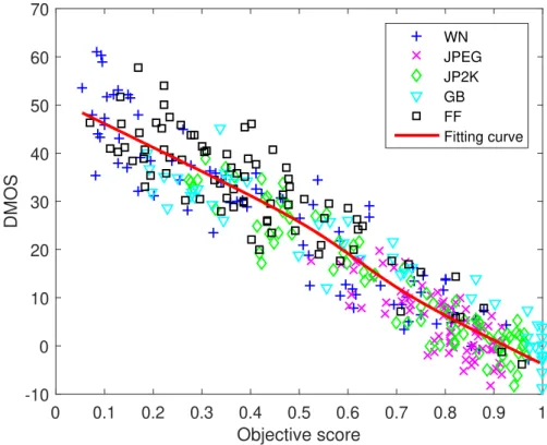
4.1 Scatter distribution of predicted scores versus DMOS on LIVE 3D phase I. . . 54
4.2 Scatter distribution of predicted scores versus DMOS on LIVE 3D phase II. . . 55
8.2 (a) JND thresholds for difference background luminance levels Lb and disparities d from LA experiment, (b) JND thresholds for difference Lb and noise amplitudes of the left view Nl from CM experiment. (c) Average slopes of the two curves in (b) for each Lb. . . 173
List of Tables
3.1 Paper II: comparison between the 3D-JND models. . . 39
4.1 Subjective test scores: quality comparison between original 3D image and noisy 3D images produced by a 3D-JND model using 12 images from Middlebury Stereo Datasets. Note that DBJND and SSJND models are respectively our model without and with considering the visual saliency effect. The higher the average of the 3D-JND model is, the better the distortion masking ability the 3D-3D-JND is. . . 52
4.2 Performance of SIQA methods on LIVE 3D IQA database (Phase I). Italicized entries denote 2D-based IQA, and the results of the best-performing SIQA method are highlighted in boldface. . . 53
4.3 Overall performance and performances for different types of distortion of the SIQA methods on LIVE 3D-IQA Phase II database. The ranking 1st and 2nd for each
criterion are highlighted with red and blue bold texts, respectively. . . 53
4.4 SROCC values of the NR-SIQA methods on cross-database. . . 54
List of Abbreviations
2D two dimensional3,4,18,28–31,34,40,41,44,46–51,59,61
2D-JND two dimensional just noticeable difference5,25,35,38,44,45,47,49,50,56,59
3D three dimensional 3–5,9,15–20,27,28,35,37,38,40,41,43–52,55–57,59–61
3D-JND stereoscopic three dimensional just noticeable difference 4–8, 35, 37, 38, 40, 44,
45,47–52,55,56,59,60
BIQA blind image quality assessment30–32
BJND binocular just noticeable difference37,45,47,49,60
DBJND disparity-aware binocular just noticeable difference38,49,51
DMOS differential mean opinion score28,30,32,33,51 DpM depth map18,20
DsM disparity map40,49,56
FR full-reference29,30,41,42,44,49,50,59 GM gradient magnitude30,31,43–45
GMSM gradient magnitude similarity mean30,44,56
HVS human visual system4,5,9,16,17,25,29,30,37,40,41,43,47,48,50,59 IQA image quality assessment7,27–34,37,40,41,43,45,46,49–52,56,57,59
ITU international telecommunication union25,28
JND just noticeable difference4,5,25–27,30,37,38,40,44–46,48–50,55,56,59,60 JP2K JPEG 200051,52,57
LE local entropy44,45,50
LoG laplacian of gaussian9,31,43–45,50,57,59 MOS mean opinion score28,30,32,33
NN neural network30,57 NOPs non-occluded pixels38,60
Contents
NR no-reference29–32,43,44,49,50,52,57,59,61
OPs occluded pixels38,49
PCC Pearson linear correlation coefficient26,33,36 PSNR peak-signal-to-noise-ratio29
QA quality assessment4,35,48–50,52,56,61 QoE quality of experience3,17,61
RF random forest30,57
RMSE root-mean-square error33,36,52
S3D stereoscopic three dimensional3–5,7,17,18,49,56
SIQA stereoscopic image quality assessment4, 5,7,8, 27,29–31,34,36,40–52,56,57,
59–61
SROCC Spearman rank order correlation coefficient26,33,36,52
SVM support vector machine30
SVQA stereoscopic video quality assessment 52,61 SVR support vector regression30–32,43,50,57
UQI universal quality index29,40,41,49,56 VIF visual information fidelity41,49,56 VM visual masking5,25,36,47,48,56,59,60
Part I
Chapter 1
Introduction
In this Chapter, we briefly give a general introduction of this thesis including the motivation, research objectives, research questions, research directions, research methodology, and thesis outline.
1.1 Motivation
With the rapid advances in hardware technologies, stereoscopic three dimensional (S3D) multimedia has made a great progress over the past few years, and has been increasingly applied in the fields of entertainment (e.g., three dimensional (3D) cinema [1], 3D-Television (TV) [2–4], 3D games [5, 6]), education [7], and medical imagery [8]. S3D technology improves the quality of experience (QoE) [9] by providing more realistic and immersive viewing experience compared to two dimensional (2D) image/video, thanks to binocular depth cues. Various instances show that 3D is flourishing:
• 3D-TV has been very well received by viewers through Channel 9 in Australia and the British Broadcasting Corporation (BBC) in the United Kingdom.
• In China, the number of 3D cinemas is exploding counting over 6000 3D screens nationwide and this number is growing daily.
• 3D content on the Internet is increasing as well. YouTube has over 15000 3D videos that can be watched.
Although 3D became popular thanks to the immersive feeling, the development of 3D technologies has also brought some technical challenges and inconvenience [10–13]. One can notice a slow-down and even a decrease of the numbers of 3D computer screens and especially 3D-TV sold in the last months [13]. This is mainly due to 3D-related issues generated at each stage from capture, compression, storage, transmission, to display.
1. Introduction
At the capture stage, there are no-common rules [2] for creating a correct 3D content besides the numerous initiatives stemming from stereographers and not always leading to unanimity. At the stages of compression and storage, 3D content format conversion and coding may probably introduce some artifacts, which usually result in depth mismatch, texture information loss, and insufficient reality [3]. Therefore, the aforementioned artifacts and defects may cause visual symptoms to viewers such as eye strain, headache, nausea, and visual fatigue [14,15]. Furthermore, the huge volumes of S3D data produced nowadays, make the storage capacity and compression efficiency more challenging. At the display stage, if the projected 3D content is not adapted to particular factors such as display size and technology, this can lead to visual discomfort [16,17] and a significant decrease of the QoE.
1.2 Research Aims
All above-mentioned challenges and issues motivated us to focus the PhD research on two aspects. On the one hand, to effectively and efficiently compress 3D image, it is important to account for human visual system (HVS) characteristics and properties (e.g., visual sensitivity). In particular, our research aims to investigate the spatial visibility threshold based on both monocular and binoc-ular visual properties. This threshold is usually referred to as the just noticeable difference (JND), which determines the maximum distortion undetectable by human eyes. Moreover, since an accurate stereoscopic three dimensional just noticeable difference (3D-JND) model can be applied in perfor-mance improvement of 3D image compression and quality assessment (QA), this research also aims to propose a reliable 3D-JND model based on study and comparison between state-of-the-art 3D-JND models. On the other hand, aiming to provide the promising viewing experience for 3D content, per-ceptual QA for stereoscopic images is quite crucial to evaluate or optimize the performance of S3D processing algorithms/systems. Therefore, the purpose of this research is to propose accurate and efficient stereoscopic image quality assessment (SIQA) methodologies based on the investigation of binocular perception. Specifically, the most important step is to find monocular and binocular factors affecting the perceptual quality of 3D images. In addition, we need to explore and model the binocular vision properties linked to the behavior of human 3D quality judgment. Finally, the SIQA models will be proposed combining the quality-related factors and considering the binocular vision properties.
1.3 Research Questions
Based on the aforementioned aims, this PhD research focuses on two main parts: spatial visibility thresholds of the binocular perception and SIQA. Each part leads to several questions described below:
1.4. Research Direction
1.3.1 Questions related to 3D-JND
Q1 Which characteristics and properties of the HVS should be taken into account for 2D and 3D digital imaging ? (see Paper II [18])
Q2 How are the performance of the state-of-the-art 3D-JND models developed based on HVS prop-erties and characteristics ? What are the advantages, drawbacks, and applications of these models ? How to evaluate the performance of the 3D-JND models in order to select the most appropriate model for particular applications ? (see Paper I [19] and Paper II [18])
Q3 How to develop a new reliable 3D-JND model accounting for HVS visual masking (VM) effects
and depth information ? How to design the psychophysical experiment modeling VM effects and binocular disparity ? How to construct a 3D-JND model based on psychophysical data ? (see
Paper III[20])
1.3.2 Questions related to SIQA
Q4 How does the HVS judge image quality based on binocular perception ? (see Paper VII [21])
Q5 What are the most influential factors for 3D image quality and to which extent are they affected
? What are the binocular perception phenomena/effects ? And how do these effects impact the perceived quality of 3D images ? (see Paper IV [22], Paper V [23], and Paper VI [24])
Q6 What precise and reliable methodology for SIQA that accounts for both monocular and binocular
influential factors ? And how do these factors affect jointly the overall 3D quality ? (see Paper
VII[21])
The above-mentioned research questions will be answered and discussed in Chapter4, and Paper
Ito Paper VII mentioned above are summarized in Chapter 3.
1.4 Research Direction
This Section presents the research direction based on the questions given in Section1.3.
It is known that human subjects may capture left and right-eye images with different qualities due to the visual asymmetry state when observing the real world. Fortunately, the HVS has the ability to correct the acceptable quality distortions, and thus create a single cyclopean view to perceive the environment. Therefore, in order to mimic the human visual perception for S3D imaging systems, we need to figure out (1) when the HVS corrects the quality difference between left and right views, (2) what is the difference threshold below which the overall 3D image quality and depth perception are guaranteed, and (3) how to reproduce the brain visual behavior regarding binocular depth cues and image quality using perceptual models ?
1. Introduction
To deal with above-mentioned issues, we need to understand the HVS sensitivity to inter-views difference. Specifically, we propose to exploit the notion of JND to reflect the minimum changes in image’s pixel that the HVS can detect. Therefore, state-of-the-art the two dimensional just noticeable difference (2D-JND) and 3D-JND models should be reviewed and studied to propose a new and reliable 3D-JND model based on visual masking effects considered in these models. This model may probably be designed based on psychophysical experiment to measure the visibility thresholds of the asymmetric noise in the stereopair. These psychophysical experiments can also help to deeply understand the behaviors/effects of binocular perception including binocular fusion, binocular rivalry, and binocular suppression. Some bio-inspired models mimicking binocular visual behavior should be explored. These perceptual models can be used in SIQA to accurately predict the overall 3D quality because it depends not only on single-view image quality or depth quality but also on the experience of binocular visual perception. As described by [25], the visual sensitivity reveals a perceptual impact of artifacts according to the spatial characteristics. Moreover, the visual sensitivity explains the tolerance of the HVS to changes/difference of pixel values in image regions, and is related to visual attention. Therefore, the visual sensitivity is proportional to visual salience and inversely proportional to JND. Integrating the models representing the visual sensitivity in the process of perceptual IQA may allow being closer to the human quality judgment as it mimics the HVS behavior.
1.5 Research Methodology
This section presents the research methodology I undertake for this thesis. In general, the research methodology used in this thesis is based on both theoretical and empirical studies. According to two research topics addressed in the thesis, the included papers are divided into Paper I – Paper III (related to 3D-JND) and Paper IV – Paper VII (related to quality assessment).
Paper I – Paper IIfirstly conduct a theoretical study (i.e., literature review) to describe and
an-alyze the existing models, and compare them in terms of their applicability, pros, and cons. Then both papers are based on an empirical study to compare the models thanks to qualitative and quantitative experimental analysis. In addition, Paper II conducts the experiments using the data that we either create or obtain data from publicly available datasets. In general, the work in Paper I and Paper II employs a deductive research methodology as they provide a theoretical overview and analysis, then an experimental evaluation and comparison. In contrast, Paper III designs a new model using the experimental data collected from psychophysical experiments. Thus, this paper refers to the inductive study and mainly focuses on an empirical study. In addition, Paper III analyzes the data using some statistical methods, and then conducts a subjective evaluation to validate the proposed model.
The research in Paper III – Paper VII are deductive because they propose the quality metrics based on the binocular perception theory and hypothesis. Furthermore, quantitative experiments are used to evaluate the metrics performance. Therefore, Paper III – Paper VII are more empirically focused. In addition, in order to compare with other existing quality metrics, these papers conduct
1.6. Dissertation Outline
Figure 1.1–Overview of thesis outline and connection with the publications. Blue blocks denote the sections in Part I, whereas red blocks represent publications described in Part II.
primary and secondary analysis of data. Primary data refer to the results derived from our exper-iments, whereas secondary data are the data collected by other researchers. The secondary data is employed because the source code of the algorithms are not publicly available and the implementation is costly.
1.6 Dissertation Outline
This dissertation contains two parts: Part I and Part II. Part I is organized as follows:
• A general introduction including PhD research motivation, objectives, directions as well as a brief organization of this dissertation.
• A research background introducing some necessary state-of-the-art knowledge with respect to human interaction with S3D technology, statistical analysis tools for psychophysical experiments and image quality assessment (IQA). This Chapter aims to provide the reader with the necessary background to understand the content of Part II.
• A summary of each included paper issue from the PhD study. In particular, we briefly present for each paper the rationale, the framework, the results, and the major contributions.
1. Introduction
• A discussion including the thesis contributions to 3D-JND models and SIQA approaches, the personal contribution for each paper, and some remaining issues and challenges.
• A general conclusion about the conducted work and some perspectives.
Part II consists of the published and submitted papers during the PhD studies demonstrating the contributions of this work. Paper I – Paper III refer to study on 3D-JND, whereas Paper IV –
Paper VIIare related to SIQA. Figure1.1depicts the overview of this thesis organization including
Chapter 2
Background
This Chapter introduces the background of this doctoral thesis that is closely related to our work, including (1) human visual system, (2) stereoscopic 3D imaging, (2) visual psychophysics and just noticeable difference,(4) statistical tools for psychophysical experiments and (5) perceptual quality assessment of 2D and 3D images. Note that this Chapter aims to briefly provide some basic knowledge of relevant topics to ensure a better understanding to the readers.
2.1 Human visual system
HVS is a biological and psychological mechanism used to perform image processing tasks, and mainly includes brain, the nervous pathways and the eyes [27]. HVS models are often used to simplify the complex visual behaviors by simulating its characteristics and properties. In this section, we briefly describe the HVS biological organization and a general 3D model.
The human eye, represented on Figure2.1, is used to capture the image corresponding to real-world scenes. It consists of the cornea, aqueous humor, iris, lens, vitreous humor and retina that the light passes through respectively [28]. Once the images are captured by the eyes, the images are projected onto the retina located at their back of the eyes. The retina contains photoreceptors, bipolar cells, horizontal cells, amacrine cells and ganglion cells [29]. After preprocessing the image in the retina, the visual information is carried by the optic nerve from the ganglion cells to lateral geniculate nucleus, and finally to the visual cortex. Several previous studies show that lateral geniculate nucleus is significantly important for visual perception and processing [30–33]. For instance, binocular rivalry behavior of the HVS is correlated to lateral geniculate nucleus [32,33]. This inspires us to use image laplacian of gaussian (LoG) response to simulate the binocular rivalry (see Paper VI and Paper VII). Finally, the visual cortex receives the visual information from both eyes and combines it to see the real-world
2. Background
Figure 2.1 –Anatomy of the human eye [26].
in 3D. A typical psychophysical HVS model is shown in Figure2.2. The main idea is to develop a HVS model considering its characteristics and properties including color information, contrast sensitivity, and spatial masking effects. The reader may refer to [34] for more details on this HVS model.
Luminance masking Local contrast and adaptation Input image Multi-channel decomposition Color processing Masking and facilitation effects Output image Contrast sensitivity function
Figure 2.2 –Flowchart of a typical psychophysical HVS model presented in [34].
2.1.1 Depth perception
HVS can perceive the environment in three dimensions, and can be able to evaluate relative distances (i.e., depth) of objects thanks to depth perception [35–37]. Depth perception relies on various depth cues [38]. Since the relative distance can be perceived by the human with one eye or both eyes, depth cues are classified into two categories: monocular and binocular depth cues.
2.1. Human visual system
to [39,40], monocular depth cues mainly include:
• Linear perspective: creates an illusion of depth on a flat surface [39]. Two parallel lines farther to the viewer result in more converging to the vanishing point. An example is shown in Figure
2.3.
Figure 2.3 –Example of linear perspective related monocular depth cue. (@ Yu FAN)
• Aerial perspective: describes the depths of the objects based on the degradation of light lu-minance and color on the scene caused by atmospheric phenomena (e.g., fog, dust) [41]. For instance, objects that are far away from the viewer have hazy edges, lower luminance contrast and color saturation as shown in Figure2.4.
2. Background
• Interposition: estimates the relative distance of the objects by showing the objects occluding each other [42]. Specifically, a farther object is usually partially occluded by a nearer object. Figure2.5 shows an example of interposition.
Figure 2.5 –Example of interposition-related monocular depth cue. (@ Yu FAN)
• Relative size: evaluates the relative depth of the physically identical objects by comparing their sizes [43]. In particular, an object with a smaller size in the scene is farther away for the viewer than the same object with a larger size. An example of wine glasses is shown in Figure2.6.
2.1. Human visual system
• Texture gradient: provides the depth of the objects depending on their textural strength [44]. Compared to farther away objects, nearer objects have finer and sharper details of texture. Figure2.7 shows an example of lavenders at different distances.
Figure 2.7 – Example of texture gradient related monocular depth cue. (@ Yu FAN)
• Light and shadow: in the scene, they can jointly reflect the relative depth between objects [45]. For instance, the objects in the shadow are farther from the light source than those out of shadow (see Figure2.8).
2. Background
• Height in the image plane: refers to vertical positions of the objects in the scene plane. In the scene, farther objects appear higher up than nearer ones. An example of this monocular depth cue is shown in Figure2.9.
Figure 2.9 – Example of height in the scene related monocular depth cue. (@ Yu FAN)
• Defocus blur: It is related to depth of focus of the HVS [46]. Objects farther away from the viewer are generally hazier and smoother, which is exhibited in Figure2.10.
Figure 2.10– Example of defocus blur related monocular depth cue. (@ Yu FAN)
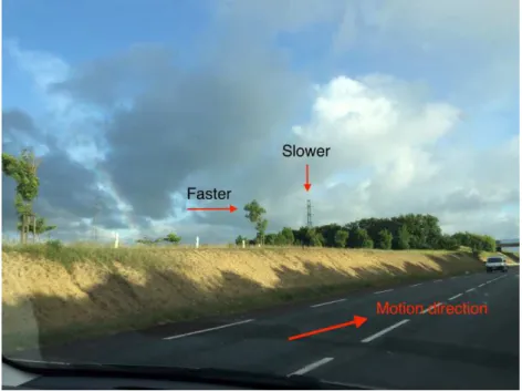
2.1. Human visual system
than farther objects [47]. Thus, this depth cue exists in a dynamic scene. Figure2.11 shows an example about motion parallax.
Figure 2.11– Example of motion parallax monocular depth cue. (@ Yu FAN)
• Accommodation: It is an oculomotor cue concerning the change of lens shape of the eyes. This change is controlled by the ciliary muscles so as to adjust the focal length [48]. Accordingly, contraction/relaxing strength of ciliary muscles can reflect the distance of the objects to the fixation point.
Binocular depth cues provide depth information when observing a scene with both eyes. There are two categories of binocular cues: binocular disparity and vergence [49,50]. Human eyes are separated by a distance of approximately 63 mm [51], which is related to parallax. Thus, for an object in the scene, both eyes can receive two similar but slightly different retinal images in terms of object’s position. This difference is defined as binocular disparity or binocular parallax [52]. As shown in Figure
2.12, the binocular disparity can be represented by either the angle difference — ≠– or horizontal shift. Another example of disparity for an object between left and right views of a stereopair is depicted in Figure 2.13. To estimate the object’s distance from viewers, human eyes extract the 3D information from texture retinal images via the binocular disparity [37,53]. This effect is named stereopsis and is generally used in the creation of 3D images/videos with specific display and/or glasses.
Another binocular depth cue is the vergence, reflecting the simultaneous movement of both eyes in opposite directions to obtain/maintain a single binocular vision [55, 56]. Specifically, eyes rotate inward when viewing a nearer object, and outward when viewing a farther object. In fact, vergence and accommodation interact intimately and cannot be separated [57–59].
2. Background
!
"
Left eye
Right eye
disparity
#
$
disparity =
# − $
Left eye
Right eye
"
!
"
!
Figure 2.12– Geometry of the binocular disparity.
Left image
Right image
Figure 2.13 –Illustration of the binocular disparity in a stereopair from the Middlebury database [54]. In addition, the objects have the same disparity if they are positioned on the corresponding locus of points in space, which is defined as the horopter [60]. In particular, horopter represents the points having the same distance from the viewer as objects of focus.
Our brain can fuse the left and right retinal images of an object into a single 3D mental image called cyclopean image [61], if this object is included in a limited area behind or in front of the horopter. This area is called Panum’s fusional area [62,63]. More details about Panum’s area can be found in [64]. Figure2.14illustrates the horopter and Panum’s area. In contrast, the image of an object outside
2.2. Stereoscopic 3D imaging
of this area is usually blurry, and thus results in binocular rivalry phenomenon due to the conflict between accommodation and vergence [65,66]. Binocular fusion behavior of the HVS occurs if the left and right views are similar in terms of content or quality [67]. In contrast, if two views are different (in terms of content or quality), and this difference is relatively small, binocular suppression occurs, one of the views dominates completely the field [68]. If this difference is relatively large, binocular rivalry occurs. Two images are seen alternately, one image dominating for a moment [65,69].
!
Left eye
Right eye
Horopter
Outer limit
Inner limit
Panum’s fusional area
Figure 2.14– Illustration of the horopter and the Panum’s fusional area.
2.2 Stereoscopic 3D imaging
The HVS can perceive the environment in 3D thanks to binocular depth cues from binocular vision. The binocular depth perception is created based on slightly different positions of two retinal images seen by left and right eyes. This difference of positions is called binocular disparity. In other words, the presentation of slightly different images to the left and right eyes leads to the perception of depth. This inspires the development of 3D technology. In this section, we introduce different 3D content representation formats and 3D displays [70].
2.2.1 S3D content representation formats
According to [71–74], there exist several S3D representation formats including: stereo interleaving, 2D-plus-depth, layered depth video, multi-view video plus depth, and depth-enhanced formats.
2. Background
Stereo interleaving format is a conventional 3D image/video format that is a multiplex of left-view and right-view images into a single image/frame. The multiplexing downsamples and places left and right images horizontally (i.e., side-by-side) or vertically (i,e., top-and-bottom). Side-by-side format was used in our psychophysical experiments (See Paper II and Paper III ). 3D video with this format can match most existing 3D codecs and displays. However, stereo interleaving format can only deliver half of the image resolution and thus reduces the QoE.
2D-plus-depth format contains a single view/frame (i.e., color image) and a depth map (DpM) for 3D image/video representation [74]. This format allows people to adjust the perceived depth values easily depending on the viewing distance and display size. However, the 2D-plus-depth format may lead to occlusion issues due to mismatches between views, and provides a limited rendering of the depth range.
To overcome the constraints of 2D-plus-depth format, the layered depth format was proposed [71, 75, 76]. In addition to the texture image and DpM, this format provides a background layer with the corresponding DpM in order to improve the occlusion information and improve the quality of depth-image-based rendering. The background layer contains image content that is covered by foreground objects in the main layer. The layered depth format allows to generate the new view points for stereoscopic and auto-stereoscopic multi-view displays.
Multi-view video plus depth format uses several cameras to capture the scene from different view points [77, 78]. Therefore, This format includes multiple color images and depth maps. The depth maps can be estimated from different views. Multi-view video plus depth format allows to control the depth range based on the distance between the selected views from the multi-view arrangement. However, this format requires large storage capacity and transmission bandwidth [79].
Depth-enhanced format includes two views with high quality, DpM and occlusion layers [80]. This format provides backward compatibility and extended functionalities such as baseline adaptation and depth-based view synthesis [71].
2.2.2 S3D displays
In order to visualize 3D images/videos, a S3D-enabled display is needed. Human subjects can perceive the spatial relationship between objects thanks to various cues including monocular and binocular cues [81]. Thus, a design of 3D displays should consider the contribution of monocular depth cues in addition to binocular depth cues in order to provide a basic visual performance as a standard 2D display and 3D sensations provided by the stereoscopic cues. Several overviews of existing 3D display technologies are provided in [77,82–85].
According to the used technology (e.g., glasses or head-mounted devices), 3D displays can be classified into three categories: stereoscopic, autostereoscopic, and head-mounted displays [82,83,86]. Stereoscopic displays are the visualization terminals that demand the observer to wear an optical device to direct the left and right images to the appropriate eye. Stereoscopic displays can be further
2.2. Stereoscopic 3D imaging
divided into:
• time-parallel displays that show left and right views of a stereopair simultaneously on the screen. In such displays, the visualization methods include: (1) color multiplexing that presents left and right images in different colors [87] ; (2) polarization multiplexing [88]. The latter uses polarized filter glasses to split left and right views ensuring that two eyes perceive different images. Linear or circular polarization can be used. The latter allows more head tilt for viewers.
In our psychophysical experiments (described in Paper II and Paper III), the Hyundai TriDef S465D display is used to convert side-by-side 3D format to 3D image by circular polarized glasses. • time-multiplexed displays that present left and right views alternately with a high frequency. Such technology generally uses active shutter glasses synchronized with the display system via an infrared link [89]. The idea is that the viewer can perceive neither the switching between left and right views nor related flicker if both views switch quickly enough (i.e., with a frequency greater than 58 Hz) [90]. Thus, based on the synchronization signal from the display, the active shutter glasses open alternately the image for one eye while closing the other.
Autostereoscopic displays do not require any glasses to present two-view images, but send them directly to the corresponding eyes using aligned optical elements on the surface of the displays [83]. This category of displays simplifies 3D perception for viewers and can show multiple views to them, which makes the 3D entertainment more applicable. In addition, autostereoscopic displays can present each view from a particular viewing angle along the horizontal direction and provide a comfortable viewing zone for each stereopair. Such displays can be classified into:
• binocular or multi-view based displays [91, 92]. Binocular views based displays only present a stereopair, whereas multi-view displays provide multiple views of the scene to several viewers based on light sources of different paths. The light paths can be controlled by special optical elements including for example parallax barriers, lenticular lens arrays, micropolarizers, etc. • head-tracked displays allowing the viewers to change the viewing position by using active optics
to track their head/pupil positions [82].
• volumetric displays generating the images by projection within a volume space instead of a surface in space. The image volume consists usually of voxels [93]. Each voxel on a 3D image is located physically at the supposed spatial position, and reflects omnidirectionally the light from that position to present a real image to viewers.
• holographic displays showing real and virtual images based on wave-front reconstruction. Such displays do not require any special glasses or external equipment to view the image. Such displays use holographic optical elements (e.g., lens, films, and beam splitter) to construct their projection screen [94,95].
2. Background
In addition to stereoscopic and autostereoscopic displays, head-mounted 3D displays are another and new way to present 3D images [86]. In particular, such displays require viewers to wear a particular head-tracking device containing sensors that record viewers’ spatial movement information. Head-mounted displays can provide the viewers with a deep feeling of immersion. Such displays have been widely advanced and applied in entertainment, education, and medical domains with virtual and augmented reality applications [96–98].
2.2.3 Depth and binocular disparity
With the aim to ease the understanding of the used depth/disparity values described in Paper II, this section describes the relationship between the depth values of 3D scene z (in meters), real-world depth map (DpM) values (in pixels) and binocular disparity values (in pixels or meters).
DpM denotes the distance of the scene’s objects from the viewpoint of the camera or the viewer. In other words, DpM represents a measure of the distance between objects in the image. DsM (Disparity map) refers to an image containing the distance values between two corresponding pixels in the left and right views of the stereo pair. A DpM map can be obtained using a 2D image, while a DsM map is only obtained using a stereopair. Note that the disparity value can be converted to depth value based on some specific formula and vice versa.
Typically, DpM and DsM is a 8-bit gray scale image. This map represents closer and farther objects with regards to the fixation plan by larger and smaller values, respectively. The depth image values vary between 0 and 255. Accordingly, the closest and farthest objects to the fixation point are shown as white and black pixels in depth images. Using the actual depth value z, the depth in pixel of DpM zp is determined as follows:
z
p=
W
W
W
U
255 ·
!
1 z≠ 1 zmax"
1
1 zmin≠ 1 zmax2
X
X
X
V
,
(2.1)where zmin and zmaxrespectively denote the minimal (closest objects) and maximal (farthest objects)
distances in the scene to the camera/observer. Both distances are usually given by 3D content maker. In addition, Â·Ê rounds the number to the lower integer. Based on Equation 2.1, the actual depth value z can be obtained from the DpM value zp using the following equation:
z = 5 z p 255· 3 1 zmin ≠ 1 zmax 4 + 1 zmax 6≠1 . (2.2)
Besides, disparity values d are frequently used to synthesize the cyclopean view for stereoscopic image quality assessment. The disparity values of a scene d are obtained by converting the depth value as
2.3. Psychophysics and just noticeable difference follows: d = f · b z = f · b · 5 z p 255· 3 1 zmin ≠ 1 zmax 4 + 1 zmax 6 , (2.3)
where b represents the distance between the stereoscopic cameras (i.e., baseline) or interpupillary distance (approximately 63mm) for viewers. Disparity values are in pixels/meter depending on the camera focal length f in pixels/meter.
2.3 Psychophysics and just noticeable difference
This section presents some basic concepts of visual psychophysics and notion of the just noticeable difference with respect to 2D and 3D images. In addition, we briefly introduce the psychophysical experiments used in our JND measurements and modeling.
2.3.1 Visual psychophysics
Visual psychophysics quantitatively study the relationship between the physical stimuli and human sensations and perceptions [99]. Specifically, visual psychophysics refers to experimental methodolo-gies that can be applied to study how to model the human visual process. The empirical laws of psychophysics are based on sensory threshold (i.e., visibility threshold) measurement by conducting psychophysical experiments [100]. Such a threshold corresponds to the point of intensity at which the observers can just detect the presence of a stimulus or the presence of a change between two stimuli.
According to [100], the visibility thresholds are classified into two types as described below. • Absolute threshold: is the minimum intensity of a stimulus that subjects can detect at least 50%
of the time.
• Difference threshold: is the minimum change/difference in intensity between two stimuli that subjects can detect usually 50% of the time. Thus this threshold is also called just noticeable difference (JND) threshold. To measure the JND threshold, a pair of stimuli is usually presented to subjects. One stimulus has a standard intensity and is considered thus as a reference. For the other stimulus, subjects vary its intensity until they can just barely inform that this stimulus is either more intense or less intense than the reference one.
Note that the visibility thresholds measurement presented in Paper II and Paper III) refers to JND thresholds. In fact, [100] states that absolute and difference thresholds are occasionally considered similar in principle because there is always background noise altering observers ability to notice stimuli.
2. Background
2.3.2 Just noticeable difference threshold
Tell when observers perceive changes in pixel values of targeted image block (represented by a green rectangular): visibility thresholds of the pixels.
Pristine image
Observer’s response: No No Yes
Images locally distorted by white noise with different levels
Just noticeable difference (JND): minimum change of a visual stimulus
Figure 2.15 –Example of JND thresholds of the pixels in an image block.
For a 2D image, the JND of a pixel represents the visibility threshold at which human subjects are able to detect changes in pixel values. In other words, the 2D-JND reflects the maximum tolerable changes in pixel intensity to HVS. Figure2.15illustrates the procedure of obtaining the JND thresholds of the pixels in a 2D image block. The subjects compare the intensity difference between the pristine image and each distorted image in the targeted block (i.e., noised region). The noise level is gradually increased until the subjects report that they just detect the difference. This difference corresponds to JND thresholds of the pixels in the block.
To date, numerous 2D-JND models have been proposed by modeling contrast sensitivity, visual masking effects (e.g., luminance adaptation and contrast masking), and spatial frequency of the image local regions [101]. Any changes in the targeted image are undetectable by the HVS if they are lower than the JND threshold. Therefore, the 2D-JND models have been successfully applied to improve the algorithms of image coding, image quality assessment and enhancement. A 3D-JND model usually estimates the maximum changes in the image region that can be introduced in one view of the stereopair without causing binocularly visible differences, given the changes in the corresponding region of the other view. Therefore, as shown in Figure2.16, in addition to monocular visual masking, the design of a 3D-JND model definitely considers the binocular vision properties (e.g., binocular masking, depth masking, and depth information). The readers can refer to Paper III for more details on 3D-JND models.
2.3. Psychophysics and just noticeable difference S3D image Contrast sensitivity, monocular visual masking Binocular visual masking, depth information Pre-processing JND profile of a single-view image
Figure 2.16– A general framework of a computational 3D-JND model.
2.3.3 Psychophysical experiments
To measure JND thresholds, a general methodology is to conduct the psychophysical or psycho-visual experiments to determine whether the subjects can detect a stimulus, or notice the difference between two stimuli. As described in [100], psychophysical experimental methods used in JND measurements are:
• Method of limits: For ascending method of limits, given a stimulus (as the reference) with the property of a constant level, the property of the targeted stimulus starts out at a low level so that the difference between this stimulus and reference one could be undetectable. Then, this level is gradually increased until the subjects report that they are aware of the difference. The JND threshold is defined as the difference level of the stimulus property for which the targeted stimulus is just detected. In the experiments, the ascending and descending methods are used alternately, and the final JND threshold is obtained by averaging the thresholds of both methods. These methods are efficient because the subjects can obtain a threshold in a small number of trials. In addition, one do not need to know where the threshold is at the beginning of the experiments. Nevertheless, two disadvantages may be observed. First, the subjects may get accustomed to informing that they detect a stimulus and may continue reporting the same way even beyond the real threshold (i.e., errors of habituation). Second, subjects may expect that the stimulus will become detectable or undetectable, and thus make a premature judgment (i.e., the error of expectation).
To overcome these potential shortcomings, a staircase (i.e.,up-and-down) method is introduced [102]. It usually starts with a stimulus having a high intensity, which is obviously detected by subjects. They give the response (’yes’ or ’no’). Then, the intensity is reduced until the subjects response changes. After that, a reversal procedure starts and the intensity is increased (with the response ’no’) until the response changes to ’yes’. Next, another reversal procedure is repeated until a given reversal number is reached. The JND threshold is then estimated by averaging the values of the transition points (i.e., reversal points).
• Method of constant stimuli: In this method, a constant comparison stimulus with each of the varied levels (ranging near the threshold) is presented repeatedly in a random order to subjects. The proportion of times causing the difference threshold is recorded. The stimulus level yielding a discrimination response in 50% of the time is considered as the JND threshold. The subjects can not predict the level of the next stimulus in the experiment. Therefore, the advantages of
2. Background
this method are to reduce errors of habituation and expectation probably caused in the method of limits. However, this method is costly because it takes a lot of trials to pre-define the levels of the stimuli before conducting the experiment. In addition, the experiment using this method is time-consuming because each stimulus needs to be presented to subjects several times. It may probably reduce the accuracy of threshold measurement due to visual fatigue during the experiment.
• Method of adjustment: In this method, a reference stimulus with a standard level is presented to subjects. They are asked to adjust the level of the targeted stimulus, and instructed to alter it until it is the same as the level of the reference stimulus. The error level between the targeted stimulus and the reference one is recorded after each adjustment. The procedure is repeated several times. The mean of the error values for all adjustments is considered as the JND threshold. The method of adjustment is easy to implement but produces probably some unreliable results.
In Paper II, we used the ascending method of limits to measure the JND thresholds of the test image by comparing the reference image. Note that the stimulus corresponds to the 3D images altered by different types of distortion. The staircase method was not used because the experiment for each subject may last a long time in the case of numerous stimuli. More details about experiments could be found in Paper II.
For modeling JND, the staircase method is more suitable and efficient than the method of limits. Therefore, the staircase method (reversal 4) was used for detecting the just noticeable noises in the psychophysical experiments of Paper III. More specifically, given the noise amplitude in the left view of a stereopair (i.e., reference stimulus) at different disparities and background luminance or contrast intensities, a subject adjusts the noise amplitude in the right view with ascending and then descending orders to make the noise just detectable or undetectable. The reversal procedure is repeated twice considering the trade-off between the measurement accuracy and experiments duration. The JND thresholds of the right view are estimated by averaging the difference in noise amplitude between the reference and the test stimuli at the four reversal points. More details could be found in Paper III. To compare the performance of state-of-the-art 3D-JND models, on the one hand, we evaluate the accuracy of the visibility thresholds estimation with the models (see Figure 2.17). In Paper II, we determine an interval of JND thresholds obtained from psychophysical experiments. Meanwhile, we estimate the JND thresholds using a 3D-JND model. Next, we verify whether the estimated JND threshold of each pixel is included in the corresponding interval. Finally, the percentage of accuracy of a 3D-JND model is obtained by dividing the number of pixels in the JND map included in the corresponding intervals by all pixels. On the other hand, we evaluate the performance of the image processing algorithms embedding 3D-JND. As shown in Figure2.17, the 3D-JND can be used in depth or sharpness enhancement of 3D images [103, 104], to reduce the bit rate for 3D video coding [105], or to improve the prediction accuracy of the SIQA model [106]. The main idea is to evaluate the
2.4. Statistical tools for psychophysical experiments Validation based on psychophysical experiments 3D-JND models Perceptual quality
measure Bit-rate saving
Applications in 3D processing Accuracy of the visibility thresholds estimation
Figure 2.17– Methodology of performance comparison for 3D-JND models. perceptual quality and/or coding efficiency of processing algorithms embedding 3D-JND.
In Paper III, the proposed 3D-JND model is validated based on a subjective test and compared with other models in terms of perceptual quality at the same noise level. According to ITU-R BT.2021-1 [107], a variant of paired comparison (i.e.,stimulus-comparison) method is used in the subjective test. In particular, we use the adjectival categorical judgment method [108]. In this method, subjects assign an image to one of the categories that are typically defined in semantic terms. The categories may reflect the existence of perceptible differences (e.g., same or different), the existence and direction of perceptible differences (e.g., more, same, less). In the subjective test of Paper III, the subjects are shown two 3D images (injected with different noise levels) at a time, randomly arranged side by side. Then, they are asked to compare the left and the right views in terms of perceptual quality and provide a score depending on the comparison scale: 0 (the same), 1 (slightly better), 2 (better), 3 (much better), -1 (slightly worse), -2 (worse), -3 (much worse). The scores provided by all subjects for each stimulus are averaged to compute the mean opinion scores. These scores are then analyzed and processed with some methods described in the following section.
2.4 Statistical tools for psychophysical experiments
The visibility thresholds of the HVS can be determined by JND models, which are developed consid-ering VM effects and visual sensitivity [109–119]. A comprehensive review of VM and 2D-JND models was given in Paper II. More details related to 2D-JND models can be found in [101].
In this section, we introduce some statistical methods for analyzing the data from psychophysical experiment or subjective test described in Paper III. An overview of the statistical tools used in image/video processing and computer vision can be found in [120]. To construct a reliable JND model using psychophysical data, we need to detect and remove the outliers related to the subjects and to the samples of each subject [121]. Some statistical methods of outliers detection have been introduced and reviewed in [122,123].
2. Background
2.4.1 Subjects-related outliers
To detect and remove unreliable subjects, a subject screening technique defined by the international telecommunication union (ITU) under the technical report BT 1788 [124] was used in Paper III. In particular, a subject is identified as an outlier if its corresponding correlation coefficient Cmin is less
than a rejection threshold. More specifically, Let Ti
j denoting the JND threshold of the jth stimulus from ith subject, where
i œ [1, N ], and j œ [1, M ]. M and N are the numbers of stimuli and subjects, respectively. Thereby the JND values from the ith subject Ti are defined as follows:
Ti= (T1i, T2i, · · · , TMi ), (2.4) and the JND values corresponding to the jth stimulus of all subjects are given by:
Tj = (Tj1, Tj2, · · · , TjN). (2.5)
Then, we define the mean vector T across all subjects as: T = (T1, T2, · · · , Tj, · · · , TM), Tj = 1 N N ÿ i=1 Tji. (2.6)
Subsequently, we calculate the correlation coefficient between Tiand T using Pearson linear correlation
coefficient (PCC) and Spearman rank order correlation coefficient (SROCC), respectively. Smaller values of P CC(Ti, T ) and SROCC(Ti, T ) are considered as Ci
min. The subject i is identified as an
outlier and discarded if the corresponding Ci
min is less than a rejection threshold RT . The latter is
calculated by: RT = I C, if C <= M CT M CT, otherwise, (2.7) where
C = |mean(Cmin) ≠ std(Cmin)| , (2.8)
where MCT denotes the maximum correlation threshold, and is set to 0.7 in the implementation of Paper III according to [124]. In addition, mean(·) and std(·) are the average and the standard deviation operators, respectively.
2.4.2 Samples-related outliers
After detecting and removing unreliable subjects, we further perform the rejection of outlier sam-ples/observations for each subject. To achieve this goal, a median absolute deviation (MAD) method and the turkey fence method can be used depending on the distribution of the subject’s observations [123]. These two methods are selected because they are both robust to identify the outliers when their
2.4. Statistical tools for psychophysical experiments
number represents less than 20% of all observations. MAD is used for approximately symmetric JND data distribution, whereas turkey fence method for asymmetric JND data distribution.
Based on MAD, the observation/stimulus j of a subject is labeled as an outlier if: |Ti
j ≠ Tj|
M AD > 3, (2.9)
and MADM can be calculated as
M AD = 1.4826 · med
j=1:M(|T i
j ≠ medj=1:M(Ti)|), (2.10)
where med(·) denotes the median operator and M is the number of stimuli. Based on turkey fence method, the observation s is identified as an outlier if:
Tji < (P1≠ 1.5 · IQR) or Tji > (P3≠ 1.5 · IQR), (2.11) where P1 and P3 respectively refer to the 25th and 75th percentile of all JND values for the stimulus j. IQR indicates the interquartile range of all JND values.
2.4.3 Normality validation and analysis of variance
To confirm the reliability of the JND data after outliers removal, a two-side goodness-of-fit Jarque-Bera (JB) test [125] is used to verify whether the JND data of each stimulus matches a normal distribution. JB for a stimulus is defined as follows:
JB = N 6 · (S
2+(K ≠ 3)2
4 ), (2.12)
where N is the number of observations/samples, S is the sample skewness, and K is the sample kurtosis. The null hypothesis is that the samples come from a normal distribution with an unknown mean and variance. This null hypothesis is rejected either (1) if JB is larger than the critical value of 5% (significance level), or (2) p≠value of the test is less than 5%.
Analysis of variance (ANOVA) is used to verify the statistical significance between different vari-ables [126]. ANOVA measures the difference among group means in a sample. In particular, it provides a test of whether the population means of several groups are equal.
The null hypothesis for ANOVA is that there is no significant difference between variables. p ≠ value Æ 5% rejects the null hypothesis, and indicates that there is a relationship between variables.
In fact, ANOVA is performed based on the assumptions including normality and homogeneity of variances of the data. Therefore, before carrying out ANOVA, the normality and homogeneity of variance for data distribution are checked with the Shapiro-Wilk test [127] and the Levene’s test [128], respectively.
2. Background
2.5 Perceptual quality assessment of 2D and 3D images
With the rapid advances in digital stereoscopic/3D image data, it becomes increasingly crucial to ac-curately and efficiently predict 3D image quality, which can be affected at different stages from image acquisition, compression, storage, transmission, to display. Accordingly, SIQA can be applied to evalu-ate/optimize the performance of 3D processing algorithms/systems (e.g., compression, enhancement, ...) [129–131]. The objective of IQA is to measure the perceived image quality, which is probably degraded in various ways. Therefore, a reliable SIQA method should measure the perceived quality highly correlating with the human judgment of quality.
2.5.1 Subjective IQA methods
The perceived quality of stereoscopic images can be assessed by either objective methods or subjective experiments. A comprehensive survey of subjective and objective IQA methods is recently presented in [132]. In subjective tests, the human subjects are asked to observe the test images and to give opinion scores. Since humans are the final receivers in most visual applications, subjective IQA methods can deliver reliable and referenced results. Many Subjective 2D- and 3D-IQA methods have been proposed by many international standardization organizations over the years. For instance, ITU recommended several standard subjective methodologies for quality assessment of 2D-TV and 3D-TV pictures including test methods, grading scales and viewing conditions [107, 108, 133]. According to [107,108], the subjective testing methods can be usually classified into three categories: single-stimulus methods, multiple-stimulus methods, and paired comparison or stimulus comparison methods. For single-stimulus methods, only one test image is shown to subjects at any time instance and is given ratings to blindly reflect its perceived quality. For multiple-stimulus methods, several images are presented to subjects simultaneously, and the subjects rank all images based on their relative perceived quality. Finally, for paired comparison methods, a pair of images are shown either simultaneously or consecutively, and the subjects are asked to choose the one of better quality.
Subjective experiments are an important tool to construct IQA databases including reference and impaired images with different types of distortions and subjective opinions for all images, represented by either mean opinion score (MOS) or differential mean opinion score (DMOS). Over the past decades, several 2D-IQA publicly available databases were proposed to advance the work of the quality assess-ment community. Examples include the laboratory for image and video engineering (LIVE) database [134], tampere image database (TID2008) [135] and (TID2013) [136] databases, categorical image qual-ity (CSIQ) database [137], LIVE multiply distorted image database (LIVEMD) [138], high dynamic range image database (HDR2014) [139], LIVE Challenge database [140], and Waterloo Exploration database [141]. More image quality databases are summarized in [142]. Subjective experiments can convincingly assess image quality and is accordingly considered as the reference results, however they are usually costly, time-consuming, and thus unsuitable for real-time application.

![Figure 2.13 – Illustration of the binocular disparity in a stereopair from the Middlebury database [54].](https://thumb-eu.123doks.com/thumbv2/123doknet/7987883.267623/33.892.126.763.633.906/figure-illustration-binocular-disparity-stereopair-middlebury-database.webp)