Improved subset simulation for the SLS analysis of two neighboring strip footings resting on a spatially random soil

HAL Id: hal-01008298

https://hal.archives-ouvertes.fr/hal-01008298

HAL is a multi-disciplinary open access archive for the deposit and dissemination of sci-entific research documents, whether they are pub-lished or not. The documents may come from teaching and research institutions in France or abroad, or from public or private research centers.

L’archive ouverte pluridisciplinaire HAL, est destinée au dépôt et à la diffusion de documents scientifiques de niveau recherche, publiés ou non, émanant des établissements d’enseignement et de recherche français ou étrangers, des laboratoires publics ou privés.

Improved subset simulation for the SLS analysis of two

neighboring strip footings resting on a spatially random

soil

Ashraf Ahmed, Abdul-Hamid Soubra

To cite this version:

Ashraf Ahmed, Abdul-Hamid Soubra. Improved subset simulation for the SLS analysis of two neighboring strip footings resting on a spatially random soil. Geo-congress 2012: State of the Art and Practice in Geotechnical Engineering, ASCE, 2012, Oakland, United States. pp.2826-2835, �10.1061/9780784412121.289�. �hal-01008298�

Improved Subset Simulation for the SLS Analysis of Two Neighboring Strip Footings Resting on a Spatially Random Soil

Ashraf Ahmed1 _{and Abdul-Hamid Soubra}2

1_{University of Nantes, Department of Civil Engineering, Bd. de l’université, BP 152,} 44603 Saint-Nazaire cedex, France. PH: (0033)240905106; FAX: (0033)240905109; email: Ashraf.ahmed@univ-nantes.fr,

2_{University of Nantes, Department of Civil Engineering, Bd. de l’université, BP 152,} 44603 Saint-Nazaire cedex, France. PH: (0033)240905108; FAX: (0033)240905109; email: Abed.Soubra@univ-nantes.fr,

ABSTRACT

The computation of the failure probability of geotechnical structures with the consideration of the soil spatial variability is generally performed using Monte Carlo Simulation (MCS) methodology. This method is very time-consuming when computing a small failure probability. As an alternative, Subset Simulation (SS) approach was proposed by Au and Beck (2001) to efficiently calculate the small failure probability. In the present paper, a more efficient approach called the improved Subset Simulation (iSS) is employed. In this approach the efficiency of SS is increased by replacing the first step of SS by a conditional simulation in which the realizations are generated outside a hypersphere of a given radius. This approach is illustrated here through the probabilistic analysis at the serviceability limit state (SLS) of two neighboring strip footings that rest on a soil with spatially varying Young’s modulus. A comparison between SS and iSS approaches has shown that a considerable reduction in the number of realizations can be achieved when using the iSS approach.

KEY WORDS: subset simulation; improved subset simulation; conditional

simulation; strip footings; differential settlement.

INTRODUCTION

The classical Monte Carlo Simulation (MCS) methodology is generally used to calculate the failure probability of problems involving a spatial variability of the soil properties. This method is very time-consuming when computing a small failure probability. This is due to the large number of realizations required in such a case. As alternative to MCS methodology, the Subset Simulation (SS) approach was proposed by Au and Beck (2001) to calculate the small failure probability. The first step of SS method is to generate a given number of realizations of the uncertain parameters using the classical MCS technique. The second step is to use the Metropolis-Hastings (M-H) algorithm to generate realizations in the direction of the limit state surface (i.e. G=0). This step is repeated until reaching the limit state surface. It should be emphasized here that in case of a small failure probability, SS requires the repetition of the second step many times to reach the limit state surface. This leads to a high

computational time. To reduce the computational cost of SS, Defaux et al. (2010) proposed an improved subset simulation (iSS) method. In this method, the efficiency of SS is increased by replacing the first step by a conditional simulation. In other words, instead of generating realizations directly around the origin by the classical MCS, the realizations are generated outside a hypersphere of a given radius. Consequently, the number of realizations required to reach the limit state surface is significantly reduced. Notice that Defaux et al. (2010) have employed the iSS to calculate the failure probability in the case where the uncertain parameters are modeled by random variables. In the present paper, the iSS is employed in the case where the uncertain parameters are modeled by random fields. This method is illustrated through the computation of the probability (Pe) of exceeding a tolerable differential settlement between two neighboring strip footings resting on a soil with a spatially varying Young’s modulus. The footings are subjected to central vertical loads with equal magnitude. The random field is discretized using the Karhunen-Loeve (K-L) expansion. The differential settlement between the two footings was used to represent the system response. The deterministic model used to compute the system response is based on numerical simulations using the commercial software FLAC.

REVIEW OF THE CLASSICAL SUBSET SIMULATION (SS) APPROACH

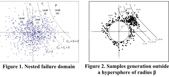
Subset simulation was proposed by Au and Beck (2001) to compute the small failure probabilities. The basic idea of the SS approach is that the small failure probability can be expressed as a product of larger conditional failure probabilities. Consider a failure region F defined by the condition G<0 where G is the performance function and let (s1, …, sk, ..., sNt) be Nt samples located in the space of the uncertain variables where s represents a vector of random variables. It is possible to define a sequence of nested failure regions F1, …, Fj, ..., Fm of decreasing size where

F F ... F ...

F₁⊃ ⊃ _j ⊃ ⊃ _m= as shown in figure 1. An intermediate failure region Fj can be defined by Gj<Cj where Cj>0. Thus, there is a decreasing sequence of positive numbers C1, …, Cj, ..., Cm corresponding respectively to F1, …, Fj,…, Fm where C1>…>Cj>...> Cm=0. The Nt samples (s1, …, sk, ..., sNt) will be divided into groups of equal number Ns of samples (s1, …, sk, ..., sNs). Thus, Nt=mxNs where m is the number of failure regions. The Νs samples of the first group are generated by MCS methodology according to a target PDF (Pt). The corresponding failure probability P(F1) is calculated as follows:

∑

F = if s∈ and F1 IF1 = otherwise. On the other hand, the samples of the 0

remaining groups are generated using Metropolis-Hastings algorithm according to a proposal PDF (Pp). The failure probability corresponding to an intermediate failure region Fj where j≠1 is calculated as follows:

∑

1 I

j

F = if s∈Fj and IFj = otherwise. The failure probability P(F) of the failure region 0

F can be calculated from the sequence of conditional failure probabilities as follows:

∏

IMPROVED SUBSET SIMULATION (iSS) APPROACH

As mentioned previously, the basic idea of iSS is to replace the first step of SS by a conditional simulation (Defaux et al. 2010) in which, the realizations are generated outside a hypersphere of a given radius β (figure 2).

Figure 1. Nested failure domain Figure 2. Samples generation outside

a hypersphere of radius β

Based on this conditional simulation, the failure probability P(F1) corresponding to the first level of subset simulation (i.e. level 0) is calculated as follows (Defaux et al. 2010):

∑

where χ_M is the chi-square distribution with M degrees of freedom and I 1

1 F = if 1 F s∈ and I 0 1

F = otherwise. The advantage of using the conditional simulation is to generate realizations in the proximity of the limit state surface leading to a reduction in the number of realizations required to reach this surface. Notice finally that the realizations of the remaining levels (i.e. levels 1 to m-1) are generated using Metropolis-Hastings algorithm. The failure probability of a given level j where j≠1 is calculated using Eq. (2) and the final failure probability P(F) is calculated using Eq. (3).

IMPLEMENTATION OF iSS IN THE CASE OF RANDOM FIELDS

As mentioned before, this paper aims at employing the iSS approach for the computation of the failure probability in the case of a spatially varying soil property. To achieve this purpose, a link between SS and K-L expansion is performed. For a Gaussian random field E(X, θ), where X denotes the spatial coordinates and θ

-5 0 5 -5 0 5 β Level 0 Level 1 Level j Level _m C1>0 Cj-1>Cj>0 Cm=G=0 F1 Fj _F

indicates the random nature of this random field, the random field can be approximated by the K-L expansion as follows (Spanos and Ghanem 1989):

) ( ) X ( ) (X, E M _{i i} 1 i i θ ξ φ λ + μ ≈ θ

∑

i

φ are the eigenvalues and eigenfunctions of the covariance function C(X1, X2), and ξi(θ) is a vector of standard uncorrelated random variables. In the present paper, the random field E was assumed to follow a log-normal probability density function so that ln(E) is a normal random field with mean value μln and standard deviation σln. For a lognormal random field, the K-L expansion given in Eq. (5) becomes (Cho and Park 2010): ⎥ ⎦ ⎤ ⎢ ⎣ ⎡_{μ + λ φ ξ θ} ≈ θ

∑

On the other hand, the random field was assumed to follow an exponential covariance function as follows:

⎟ ⎟ ⎠ ⎞ ⎜ ⎜ ⎝ ⎛ ₋ − − − σ = y ln 2 1 x ln 2 1 2 ln 2 2 1 1 _l y y l x x exp )] y , x ( ), y , x [( C (7)

where (x1, y1) and (x2, y2) are the coordinates of two arbitrary points in the domain over which the random field is defined and lln x and lln y are respectively the horizontal and vertical lengths over which the values of ln(E) are highly correlated. Notice that in the case of an exponential covariance function, the eigenvalues and eigenfunctions are given analytically. Their solutions are presented in Spanos and Ghanem (1989).

Notice that the basic idea of the link between SS and K-L expansion was given in Ahmed and Soubra (2011) and is briefly presented herein in the case of iSS approach applied to a random field problem. This link is performed through the standard normal random variables

M ..., , 1 i i}

{ξ ₌ appearing in Eq. (6) as follows: for a given random field realization discretized by K-L expansion, the system response is calculated in two steps. The fist step is to substitute the vector

M ..., , 1 i i} {ξ ₌ of this

realization in Eq. (6) to calculate the value of the random field at each point in the domain according to its coordinates. The second step is to use the deterministic model to calculate the corresponding system response. The algorithm of iSS proposed in this paper for the case of a spatially varying soil property can thus be described as follows:

1. Prescribe a radius β for the hypersphere and generate a vector of standard normal random variables {ξ1, …, ξi, ..., ξM} by MCS methodology. This vector must realize that its norm is larger than the prescribed radius β.

2. Substitute the vector {ξ1, …, ξi, ..., ξM} in the K-L expansion (Eq. 6) to obtain the first realization of the random field. Then, use the deterministic model to calculate the corresponding system response.

3. Repeat steps 1 and 2 until obtaining a prescribed number Ns of realizations and their corresponding system response values. Then, evaluate the corresponding

values of the performance function to obtain the vectorG₀ ={G1₀,...,Gk₀,...,G₀Ns}. Notice that the subscript ‘0’ refers to the first level (level 0).

4. Prescribe a constant intermediate failure probability P(Fj) for all the failure regions Fj and evaluate the first failure threshold C1 which corresponds to the failure region F1 where C1 is equal to the [(NsxP(Fj))+1]th value in the increasing list of elements of the vector G0. Thus, among the Ns realizations, there are [NsxP(Fj)] ones whose values of the performance function are less than C1 (i.e. they are located in the region F1). The failure probability P(F1) is then calculated by Eq. (4)

5. The vectors of {ξ1, …, ξi, ..., ξM} corresponding to the realizations that are located in the region F1 (from step 4) are used as ‘mother vectors’ to generate additional [(1-P(Fj))Ns] vectors of {ξ1, …, ξi, ..., ξM} using Metropolis-Hastings algorithm. These new vectors are substituted in Eq. (6) to obtain the random field realizations of level 1. Then, the values of the performance function corresponding to these realizations should be calculated and gathered in an increasing order in the vector of performance functionsG {G ,...,G ,...,GNs}

1 k 1 1 1 1 = .

6. Evaluate the second failure threshold C2 as the [(NsxP(Fj))+1]th value in the increasing list of the vector G1.

7. Repeat steps 5 and 6 to evaluate the failure thresholds C3, C4, …, Cm corresponding to the failure regions F3, F4, …, Fm. Notice that contrary to all other thresholds, the last threshold Cm is negative. Thus, Cm is set to zero and the conditional failure probability of the last level [P(Fm׀Fm-1)] is calculated as:

∑

F = if the performance function G(sk) is negative and IFm = otherwise. 0

8. Finally, the failure probability P(F) is evaluated according to Eq. (3).

EXAMPLE PROBLEM

In this section, the efficiency of the iSS is illustrated through an example problem. In this example, a probabilistic analysis at SLS of two neighboring strip footings resting on a soil with a spatially varying Young’s modulus was performed. Each footing is subjected to a central vertical load P=1000kN/m. Due to the soil heterogeneity, the two footings exhibit a differential settlement δ. This differential settlement is calculated as the absolute difference δ = δ₁ − δ₂ where δ1 and δ2 are the settlements (computed at the footing center) of the two footings. The differential settlement δ is used to represent the system response. The Young’s modulus is modeled by a random field and it was assumed to follow a log-normal distribution. Its mean value and coefficient of variation are respectively μE=60MPa and COVE=15%. It was discretized using K-L expansion. An exponential covariance function (Eq. 7) was used in this paper. Although an isotropic random field is often assumed in literature (e.g. Fenton and Griffiths 2002, 2005), the vertical autocorrelation length tends to be shorter than the horizontal one. A common ratio of about 1 to 10 for these autocorrelation lengths can be used (Baecher and Christian

2003). Notice however that in this paper, different values of autocorrelation lengths were studied and analyzed in order to explore some interesting features related to the autocorrelation lengths. The performance function used to calculate the probability (Pe) of exceeding a tolerable differential settlement is defined as follows:

δ − δ = _max

G (9)

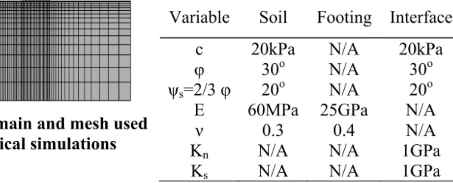
where δmax is a prescribed tolerable differential settlement and δ is the computed differential settlement due to the soil heterogeneity. The deterministic model used to calculate the differential settlement δ is based on numerical simulations using FLAC. For this computation, two footings (each of width b) were considered in the analysis (Figure 3). The two footing centers are separated by a distance D. A non-uniform optimal mesh composed of 1290 zones was employed. Although this paper presents an SLS analysis, the soil behavior was modeled by a conventional elastic-perfectly plastic model based on Mohr-Coulomb failure criterion in order to take into account the possible plastification that may take place near the footing edges even under the service loads. The strip footings were modeled by a linear elastic model. They are connected to the soil via interface elements. The values of the different parameters of the soil, footings and interfaces are given in Table 1.

Figure 3. Soil domain and mesh used in the numerical simulations

Table 1. Shear Strength and Elastic Properties of Soil, Footing, and Interface

Variable Soil Footing Interface

c 20kPa N/A 20kPa

φ 30o N/A 30o

ψs=2/3 φ 20o N/A 20o

E 60MPa 25GPa N/A

ν 0.3 0.4 N/A

Kn N/A N/A 1GPa

Ks N/A N/A 1GPa

In order to calculate the differential settlement for a given random field realization, (i) the coordinates of the center of each element of the mesh were calculated; then, Eq. (6) was used to calculate the value of the Young’s modulus at each element, (ii) geostatic stresses were applied to the soil, (iii) the obtained displacements were set to zero in order to obtain the footing displacement due to only the footings applied loads and finally, (iv) the service loads were applied to the footings and the vertical displacements at the footings centers due to these loads are calculated. The differential settlement is calculated as the absolute difference between the two footings displacements. It should be noticed that, for all the probabilistic analyses performed in this paper, a normal PDF was used as a target PDF (i.e. it was used to generate the Ns realizations of the first level). However, a uniform PDF was chosen as a proposal PDF (i.e. it was used to generate the Ns realizations of each one of the remaining levels). The intermediate failure probability P(Fi) was chosen equal to 0.1. Also, the tolerable differential settlement δmax was assumed equal to 3.5x10-3 m. It should be mentioned here that lln x and lln y were normalized with respect to the distance D between the centers of the two footings (i.e. Lln x=lln x/D and Lln y=lln y/D). The numerical results have shown that this

assumption is valid when the ratio D/b is constant. Notice that all the probabilistic results presented in this paper correspond to a ratio of D/b=2. Finally, the number of terms of K-L expansion used in this paper is M=100 terms except in the two following cases (Lln x=Llny=0.25 in case of an isotropic random field and, Lln x≤0.25 and Lln y≤0.25 in case of an anisotropic random field) where 500 terms were required.

Probabilistic results

This section presents the probabilistic results of the example problem described above. First, the number of realizations Ns to be used in the different levels of iSS has to be selected. This number must be sufficient to provide accurate Pe values. Different values of Ns were considered. For each Ns value the failure thresholds C1, C2, etc. were calculated and presented in Table 2 when the radius β is equal to zero. This table shows that the value of the failure threshold decreases with the successive levels until reaching a negative value at the last level.

Table 2. Evolution of the Failure Threshold with the Different Levels of the iSS

and with the Number of Realizations Ns (β=0, Lln x=2.5 and Lln y=0.25)

Failure threshold Cj for each

level j

Number of realizations at each level (Ns)

200 400 600 800 1000 1200 C1 0.00191 0.00199 0.00189 0.00204 0.00191 0.00195

C2 0.00103 0.00099 0.00096 0.00110 0.00102 0.00103

C3 0.00041 0.00032 0.00021 0.00037 0.00036 0.00034

C4 - 0.00009 - 0.00051 -0.00036 - 0.00037 - 0.00039 - 0.00038 For each Ns value presented in Table 2, Pe corresponding to each level j was calculated by iSS as follows:

) ( ... ) ( ) ( ) (F_j =P F₁ xP F₂F₁ x xP F_j F_j−1 P (11)

These Pe values were compared to those computed by the crude MCS methodology using a number N=30,000 realizations (Figure 4). Notice that at a given level j, the Pe value is calculated by MCS methodology as follows:

∑

in which, Gk is the value of the performance function at the kth realization and IF=1 if Gk<Cj and IF=0 otherwise. The comparison has shown that for Ns=1,000 realizations, the Pe value computed by iSS at the different levels is very close to that computed by the crude MCS methodology. Thus Ns=1,000 realizations will be used in all the probabilistic analyses performed in this paper. Notice that when Ns=1,000 realizations, the coefficient of variation of Pe by iSS is COVPe=31.5%. However, COVPe by MCS methodology using 30,000 realizations is equal to 31.3%. Notice also that when β=0, four levels of SS were required to reach the limit state surface G=0. This means that a total number of realization Nt=1,000+(900x3)=3,700 realizations were required to calculate Pe. Thus, for the same accuracy, the number of realizations (and consequently, the computation time) is reduced by 87.7% with

respect to MCS when β=0. (i.e. when the classical SS is used). This number can be again reduced by increasing β (i.e. by using iSS). Table 3 shows that, when β increases, the total number of realizations decreases. When β=11.5, only 2 levels are required. Thus, the total number of realizations is Nt=1000+900=1,900 realizations.

0.0001 0.001 0.01 0.1 1 0 0.0005 0.001 0.0015 0.002 C Pe SS (Nt=2,220 realizations) MCS (Nt=30,000 realizations)

a. Ns=600 realizations per level

0.0001 0.001 0.01 0.1 1 0 0.0005 0.001 0.0015 0.002 0.0025 C Pe SS (Nt=2,960 realizations) MCS (Nt=30,000 realizations)

b. Ns=800 realizations per level

0.0001 0.001 0.01 0.1 1 0 0.0005 0.001 0.0015 0.002 C Pe SS (Nt=3,700 realizations) MCS (Nt=30,000 realizations)

c. Ns=1000 realizations per level

Figure 4. Comparison between Pe computed by iSS and that computed by MCS

methodology at each level of iSS (β=0, Lln x=2.5 and Lln y=0.25).

As a conclusion, the number of realizations (and consequently, the computation time) required by SS approach could be reduced by 48.6% by employing the iSS approach.

Table 3. Effect of the Radius of the Hypersphere on the Number of Realizations Required to Calculate Pe (Lln x=2.5 and Lln y=0.25)

MCS _{(Classical SS)}β=0 iSS

β=10 β=11 β=11.5

Pe (x10-4) 3.40 3.65 3.58 3.36 3.45

Number of levels - 4 3 3 2

number of realizations 30,000 3,700 2,800 2,800 1,900 computation time (minutes) 210,000 25,900 19,600 19,600 13,300

Effect of the autocorrelation length on Pe in the case of an isotropic random field

Figure 5 shows the effect of the autocorrelation length on the Pe value in the case of an isotropic random field. This figure indicates that Pe presents a maximum value when Lln x=Lln y=1. This can be explained by the fact that when the autocorrelation lengths are very small, one obtains a highly heterogeneous soil in both the vertical and the horizontal directions with a great variety of high and small values of the Young’s modulus beneath the footings. In this case, the soil under the footings contains a mixture of stiff and soft soil zones. Due to the high rigidity of the footings, their movements are resisted by the stiff soil zones. This leads to a small value of the footings displacements (i.e. to a small differential settlement) and thus, to a small value of Pe. On the other hand, when the autocorrelation lengths are large, the soil tends to be homogenous. This means that the differential settlement tends to be very small (close to zero) which leads to a very small value for Pe. For the intermediate values of the autocorrelation lengths corresponding to (Pe)max, there is a high probability that one footing rests on a stiff soil zone and the other on a relatively soft soil zone. This leads to a high differential settlement and thus to a high Pe value. This configuration corresponds to the case where Lln x=Lln y=1.

0.00001 0.0001 0.001 0.01 0.1 0 2 4 6 8 10 12 14 Lln x=Lln y Pe

Figure 5. Effect of the autocorrelation lengths on Pe (isotropic random field)

Effect of the autocorrelation lengths on Pe in the case of anisotropic random field

Figures 6 shows the effect of Lln x on Pe when Lln y=0.25. This figure shows that Pe presents a maximum value when Lln x=1. For the very small values of Lln x compared to Lln y, one obtains a vertical multilayer composed of thin sub-layers where each sub-layer may have a high or a small value of the Young’s modulus. The sub-layers with high values of the Young’s modulus prevent the movements of both footings and thus lead to a small value of Pe. On the other hand, when Lln x is very large compared to Lln y, one obtains a horizontal multilayer (case of a one-dimensional vertical random field) for which each sub-layer may have a high or a small value of the Young’s modulus. This leads to the same displacement for both footings and thus to a very small value of Pe. Finally, when Lln x is equal to 1, the horizontally extended stiff layers become less extended and thus one obtains a greater differential settlement and consequently a greater value of Pe.

0.0000001 0.000001 0.00001 0.0001 0.001 0.01 0.1 0.00 2.00 4.00 6.00 8.00 Lln x Pe

Figure 6. Effect of Lln x on Pe when

Lln y=0.25 0.00001 0.0001 0.001 0.01 0.1 0 5 10 15 20 25 Lln y Pe One-dimensional

random field Two-dimensional random field

Figure 7. Effect of Lln y on Pe when

Lln x=2.5

The effect of Lln y is presented in Figure 7 when Lln x=2.5. This figure shows that the Pe value increases with the increase in Lln y. This can be explained as follows: when Lln y is very small, the two footings rest on a horizontal multilayer composed of thin sub-layers where each sub-layer may have a high or a small value of the Young’s modulus. This means that δ1 and δ2 are almost equal. Thus, the differential settlement δ is very small which results in a small value of Pe. On the other hand, when Lln y is very large, the soil tends to the case of a one-dimensional horizontal random field. In

this case, one obtains vertically extended stiff sub-layers adjacent to vertically extended soft sub-layers. For the chosen value of Lln x, there is a high probability that one footing rests on a vertical stiff layer and the other one rests on a vertical soft layer which leads to a high differential settlement and thus to a great value of Pe.

CONCLUSION

This paper presents an efficient method to perform a probabilistic analysis of geotechnical structures that involve spatial variability. This method is an improvement of the classical subset simulation approach to calculate the small failure probabilities using a reduced number of realizations. It was illustrated through an example problem in which, a probabilistic analysis at SLS of two neighboring strip footings was performed. The footings rest on a soil with a spatially varying Young’s modulus. The proposed procedure has significantly reduced the number of realizations required by the classical subset simulation approach to calculate the probability Pe of exceeding a tolerable differential settlement. A parametric study to investigate the effect of the autocorrelations lengths on Pe has shown that: (i) in case of an isotropic random field, Pe presents a maximum value when the autocorrelation lengths are equal to the distance between the footings centers, (ii) in case of an anisotropic random field, for a given Lln y value, Pe presents a maximum when Lln x=D. However, for a given value of Lln x, Pe increases with the increase in Lln y and then it attains an asymptote corresponding to the case of a one-dimensional random field.

REFERENCES

Ahmed, A., Soubra, A.-H., (2011). “Subset simulation and its application to a spatially random soil.” GeoRisk 2011, June 26-28, Atlanta, Georgia:209-216. Au, S.K., and Beck, J.L. (2001). “Estimation of small failure probabilities in high

dimentions by subset simulation.” Journal of Probabilistic Engineering

Mechanics, 16: 263-277.

Baecher, G.B., and Christian, J.T. (2003). “Reliability and Statistics in Geotechnical Engineering.” New York: Wiley.

Cho, S.E., and Park, H.C. (2010). “Effect of spatial variability of cross-correlated soil properties on bearing capacity of strip footing.” International Journal for

Numerical and Analytical Methods in Geomechanics, 34: 1-26.

Defaux, G., Meister, E., and Pendola, M. (2010). “Mécanique probabiliste et intégrité des cuves des réacteurs nucléaires.” JFMS’10, Toulouse, France: 23 pages Fenton, G.A., and Griffiths, D.V. (2002). “Probabilistic foundation settlement on a

spatially random soil.” Journal of Geotechnical and Geoenvironmental

Engineering, ASCE, 128(5): 381-390.

Fenton, G.A., and Griffiths, D.V. (2005). “Three-dimensional probabilistic foundation settlement.” Journal of Geotechnical and Geoenvironmental

Engineering, ASCE, 131(2): 232-239.

Spanos, P.D., and Ghanem, R. (1989). “Stochastic Finite Element Expansion for Random Media.” Journal of Engineering Mechanics, ASCE, 115(5): 1035-1053.