HAL Id: hal-00069802
https://hal.archives-ouvertes.fr/hal-00069802
Submitted on 19 May 2006
HAL is a multi-disciplinary open access
archive for the deposit and dissemination of
sci-entific research documents, whether they are
pub-lished or not. The documents may come from
teaching and research institutions in France or
abroad, or from public or private research centers.
L’archive ouverte pluridisciplinaire HAL, est
destinée au dépôt et à la diffusion de documents
scientifiques de niveau recherche, publiés ou non,
émanant des établissements d’enseignement et de
recherche français ou étrangers, des laboratoires
publics ou privés.
Modular Verification for a Class of PLTL Properties
Pierre-Alain Masson, Hassan Mountassir, Jacques Julliand
To cite this version:
Pierre-Alain Masson, Hassan Mountassir, Jacques Julliand. Modular Verification for a Class of PLTL
Properties. 2000, pp.398-419. �hal-00069802�
ccsd-00069802, version 1 - 19 May 2006
Modular Verification for a Class of P LT L
Properties
Pierre-Alain Masson, Hassan Mountassir, and Jacques Julliand
LIFC - Laboratoire d’Informatique de l’universit´e de Franche-Comt´e 16, route de Gray, 25030 Besan¸con Cedex
Ph:(33) 3 81 66 64 52, Fax:(33) 3 81 66 64 50
{masson,mountass,julliand}@lifc.univ-fcomte.fr Web : http://lifc.univ-fcomte.fr
Abstract. The verification of dynamic properties of a reactive systems by model-checking leads to a potential combinatorial explosion of the state space that has to be checked. In order to deal with this prob-lem, we define a strategy based on local verifications rather than on a global verification. The idea is to split the system into subsystems called modules, and to verify the properties on each module in separation. We prove for a class of P LT L properties that if a property is satisfied on each module, then it is globally satisfied. We call such properties mod-ular properties. We propose a modmod-ular decomposition based on the B refinement process.
We present in this paper an usual class of dynamic properties in the shape of 2(p ⇒ Q), where p is a proposition and Q is a simple temporal formula, such as q, ♦q, or qUr (with q and r being propositions). We prove that these dynamic properties are modular. For these specific patterns, we have exhibited some syntactic conditions of modularity on their corresponding B¨uchi automata. These conditions define a larger class which contains other patterns such as 2(p ⇒ (qUr)).
Finally, we show through the example of an industrial Robot that this method is valid in a practical way.
Keywords.Refinement, modularity, Verification, model-checking, B¨uchi automata, Propositional linear temporal logic P LT L, B specification.
1
Introduction
This paper is about the problem of the verification of finite reactive systems [18, 3, 4]. The work that we present takes the B events system specification as a context [1], in which we introduce and verify dynamic properties of liveness and safety [16, 17].
A solution for the verification of dynamic properties is to use a model- checker [10, 11]. In comparison with proof techniques, such an approach offers the ad-vantage of a possible and entire automatization, without the use of variants and loop invariant. The well known inconveniences of it are its limitation to finite
state systems and the potential combinatorial explosion of the number of states to be checked.
The problem of combinatorial explosion has been treated through various methods with time or memory space gain as a result. Let us cite by the way the memory compression techniques [12], the partial verification techniques based on heuristics [9], the memory efficient algorithms [6], the partial order techniques [21, 8] suppressing useless interleaving, the techniques of symbolic representation of the states with BDD and the techniques of state vector abstraction [7].
The approach that we expand below, based on the verification by model-checking, attacks the problem of the combinatorial explosion in a different way. We use a decomposition of the reachability graph into several modules. We then verify the properties module after module. We prove that an interesting class of P LT L properties can be verified modularly. In others words, if the property holds on every module, we prove that it holds on the whole system.
All the decompositions are not equivalent. For some decompositions and for dynamic properties that can be verified in a modular way, the modular verifi-cation is valid whereas for some other decompositions, the modular verifiverifi-cation might fail even when a property is true. Thus, the problem consists in finding a “good” decomposition. We use the notion of refinement induced by the B method to produce the modular split. The refinement of an abstract model by a concrete one induces a split of the concrete graph into subgraphs, according to the structure of the abstract graph. On such subgraphs, a modular verification is valid.
As a matter of fact, the B refinement process introduces new dynamic prop-erties at each level of the refinement, together with the new events to which they are linked. So, the decomposition by refinement “keeps” the sequences of new events within subgraphs. This is the reason why such a split, which relies on a partition of the state space, is a “good” modular split. In other words, the refinement process produces a semantic split.
Some other modular approaches have been proposed that use compositional verification [13]. They are based on the parallel operationality which allows to split the model into components that contribute to the entire state space in a multiplicative way. Our approach splits the model of a component in an addi-tive way. Since on one hand the B refinement allows the expression of parallel composition and, on the other hand, it preserves all the P LT L properties but the ones that contain the next operator, the two techniques are compatible. It is possible to verify separately a process component with a modular approach in the sense of our proposition.
Conversely, in [15], Karen Laster and Orna Grumberg present a modular ap-proach in our sense to temporal logic model-checking of software, in which a pro-gram text is partitioned into sequentially composed subpropro-grams. The model-checking is then performed on each subprogram, separately but not indepen-dently. As a matter of fact, some information (by means of an assumption func-tion) needs to be transmitted from one module to another. This is due to the fact that the partition proposed is a syntactic one.
Based on the refinement, the modularity that we propose is a semantic one. Furthermore, our modular approach is compatible with the use of the techniques that reduce the combinatorial explosion mentioned above.
Section 2 describes the concept of modular verification. In section 3, we define a class of dynamic properties by means of B¨uchi automata, and we prove that the properties in this class can be verified in a modular way. Section 4 defines the refinement relation between the abstract and refined specifications in B. To illustrate this work, we give in section 5 a simple example of an industrial Robot in order to exhibit the abstract and detailed specifications with their P LT L properties. Finally, we conclude this work and give some future directions of research.
2
Modular Verification
2.1 Principle of the Modular Verification
The basic idea of the modular verification is simple. Since a transition system might be too large to be verified by model-checking in an exhaustive way, we shall split it into several smaller pieces called modules in order to perform the verification on each module in separation.
Notice that every state and transition of the original transition system must belong to one module at least, so that the modular split must consist of a par-tition for the transitions and of an overlapping for the states, that are possibly both the target of a last transition of a module and the source of a first transition of another module.
Thanks to the modular split, a property can then be verified by model-checking on each module in separation, so that it is never necessary to keep the whole transition system in memory. With such a verification, we want to be able to tell whether the property is globally true or not.
2.2 Modular Property
When a property is true on every module, it is not always possible to conclude that it is globally true. Further in this section, we look at the P LT L property pattern 2(p ⇒ 2q) which is possibly true on every module although globally false. Thus, we have to distinguish the properties that can be verified in a mod-ular way and the ones that can not. We will say that a P LT L property P is modular if and only if
P true on every module ⇒ P globally true.
We will give a formal definition of a modular property in definition 4.
Thus, given a specification with dynamic properties in P LT L, we first have to make sure that these properties are modular before we verify them in a modular way. Section 3.3 shows that the three P LT L property patterns 2(p ⇒ q),
2(p ⇒ ♦q) and 2(p ⇒ qUr), where p, q and r are propositional formulae over the states of a transition system, are modular.
Notice that
P true on every module ⇒ P globally true is equivalent to
P globally false ⇒ P false on one module at least.
Thus, in order to detect the modularity of a property, we will suppose that this property is globally false. If we can prove that in this case it also false on a module, then we know that the property is modular.
As examples, let us look at the two property patterns 2(p ⇒ ♦q) and 2(p ⇒ 2q). The first pattern is modular, as will be proved in section 3.3. The second pattern is not modular. In both cases, we suppose that the properties are globally false. That is, we consider sequences that satisfy the negations of the properties. The modular split will possibly “cut” the sequences, and so we look whether the cut sequences still negate the properties or not.
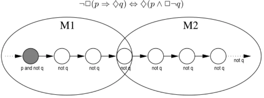
A Modular Property: 2(p ⇒ ♦q) Let us suppose that the property P = 2(p ⇒ ♦q) is globally false. Then, the negation of the property is true. Notice that ¬P is equivalent to ♦(p ∧ 2¬q). This means that there is a sub-sequence satisfying p ∧ 2¬q. Fig. 1 shows such a sequence, and how it is cut by a two modules split.
¬2(p ⇒ ♦q) ⇔ ♦(p ∧ 2¬q)
p and not q not q not q not q not q not q not q not q
M1
M2
Fig. 1.Modular property 2(p ⇒ ♦q)
In module M2, there is no state satisfying p and so P is trivially true in
this module. In module M1, a state satisfies p which is followed by states all
satisfying ¬q. As a consequence, P is indeed false in this module.
This is due to the fact that, with property pattern 2(p ⇒ ♦q), once a state satisfying p has occurred, a response (in the shape of a state satisfying q) is waited for. If this response never comes (2¬p), one may cut the sequence, it still will not come.
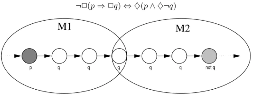
A Non-modular Property: 2(p ⇒ 2q) Let us suppose that the property P = 2(p ⇒ 2q) is globally false. Then, the negation of the property is true. Notice that ¬P is equivalent to ♦(p ∧ ♦¬q). This means that there is a sub-sequence satisfying p ∧ ♦¬q. Fig. 2 shows such a sub-sequence, and how it is cut by a two modules split.
¬2(p ⇒ 2q) ⇔ ♦(p ∧ ♦¬q)
M1
M2
p q q q q q not q
Fig. 2.Non-modular property 2(p ⇒ 2q)
In module M2, there is no state satisfying p and so P is trivially true in
this module. In module M1, the state satisfying p is now followed by states all
satisfying q, so that this cut sequence no longer negates P . As a consequence, P is possibly true in that module as well, although it is globally false.
This is due to the fact that, once a state satisfying p has occurred, the sequence remains possibly true as long as a state satisfying ¬q has not occurred. If the sequence is cut before that state, then it possibly satisfies P .
3
Verification of the Modularity
Before we perform a modular verification, we have to prove that the dynamic properties that we want to verify are modular.
In this section, we are looking at a class of dynamic properties defined from the B¨uchi automata [20] that recognize their negation. We call this class BA2.
We prove that every property in the class BA2 is a modular property.
As examples of properties that belong to the class BA2, we prove that,
amongst others, the dynamic properties suggested by the three patterns of dy-namic constraints introduced by J.-R. Abrial in [2] are modular. They consist in the three following patterns of P LT L properties: 2(p ⇒ q), 2(p ⇒ ♦q) and 2(p ⇒ pUq) where p and q are propositional formulae over the states of a transition system.
Let P be a P LT L property. We have ever noticed that we prove P modular equivalently by proving that if P is false on the whole transition system, then it is false on one module at least. For this we consider the B¨uchi automaton that recognizes the negation of P . We know that every path σ in the whole graph that
negates the property is recognized by this automaton. We then prove that there is a part of such a path σ that belongs to one module and that is recognized by the B¨uchi automaton. This proves that the property is false on that module. 3.1 Definitions for the Verification of the Modularity of Dynamic
Properties
In this section, we introduce the notations and the definitions that we use to establish that the three above patterns are modular.
Definition 1 (Transition System) A transition system is a 6-tuple T S = < A, S, S0, →, AP, L > where A is an alphabet labelling the transitions, S is the
set of states, S0 ⊆ S is the set of initial states, → is the transition relation
(→⊆ S ×A×S), AP is a set of propositions and L : S 7→ 2AP is the assignment
function.
Let T S =< A, S, S0, →, AP, L > be a transition system. Let us consider a
partition of the set S of states. Each part of the partition can be regarded as an equivalence class EQi such that S =
[
i
EQi. Some states in EQi are the
source states of some transitions in → whose target states are not in EQi. We
call these transitions the exiting transitions of EQi. A module M of a transition
system T S is a transition system whose set of states is composed of the states in EQi augmented with the target states of the exiting transitions.
Definition 2 (Module) Let T S =< A, S, S0, →, AP, L > be a transition
sys-tem. Let PS be a partition of S. Each equivalence class EQ of PS allows the
def-inition of a module which is a transition system T S′
=< A, S′ , S′ 0, → ′ , AP, L′ > defined in the following way:
– S′= EQ ∪ {s ∈ S/∃s 1
a
→ s ∈→ ∧s1∈ S1∧ s /∈ S1}
S′
is the set of states of the class augmented with the exiting states, – →′= {s
1 a
→ s ∈→ /s1∈ S′∧ s ∈ S′}
→′ is the set of transitions that link the states of S′,
– S′ 0= {s ′ ∈ S′ /∃s→ sa ′ ∈→ ∧s→ sa ′ / ∈→′ } S′
0 is the set of states of S ′
reachable from a transition in → that is not in →′
,
– L′ is the restriction of L on S′.
We call internal states the states of the modules that are in EQ, whereas we call exiting states the target states of the exiting transitions. With such a definition, we have indeed a partition of the transitions of T S and an overlapping of the states of T S.
Notations 3 Let P be a dynamic property in P LT L and T S a transition sys-tem. We denote T S ⊢ P the fact that the property P is satisfied on T S. Its meaning is defined by the semantics of P LT L. We denote s |= p the fact that a state s satisfies a boolean proposition p. Thus, we have s |= p iff p ∈ L(s).
Given a P LT L property P , a transition system T S and its split into a set M of modules M , we want to prove that P is modular.
Definition 4 (Modular Property) Let P be a P LT L property. Let M be the split of a transition system T S into modules. The property P is modular iff
(∀M ∈ M, M ⊢ P ) ⇒ T S ⊢ P which is equivalent to
T S 0 P ⇒ ∃M ∈ M ∧ σ path of M s.t. σ ⊢ ¬P .
Definition 5 (Path of a Transition System) A path σ = s0s1. . . si. . . of a
transition system T S =< A, S, S0, →, AP, L > is defined as a sequence (finite or
infinite) of states linked by a transition.
∀si ∈ σ, si+1 ∈ σ, ∃t ∈→ s.t. t = si→ si+1 .
Definition 6 (B¨uchi Automaton) A B¨uchi automaton is a 5-tuple B = < b0, B, AP, →B, Accept > where:
– b0 is the initial state,
– B is the finite set of states (b0∈ B),
– AP is a set of boolean propositions (the labels of the transitions),
– →B is the finite set of transitions labeled by propositions of PB : →B⊆ B ×
AP × B,
– Accept ⊆ B is the set of accepting states of the automaton.
Remark. A B¨uchi automaton is defined as a transition system in which we distinguish accepting states, and whose transitions are labeled with boolean propositions. As the states of a B¨uchi automaton are not valued, we need not introduce the assignment function L in its definition.
Definition 7 (Recognition of a Finite Path) A finite path σ = s0s1. . . sn
of a transition system T S =< A, S, S0, →, AP, L > is recognized by a path τ =
b0b1. . . bn+1 of a B¨uchi automaton B =< b0, B, AP, →B, Accept > if and only if
i) ∀i, 0 ≤ i ≤ n, si∈ σ ⇒ ∃pi∈ AP s.t. bi pi
→ bi+1∈ TBand si|= pi
ii) bn+1∈ Accept
Definition 8 (Recognition of an Infinite Path) An infinite path σ = s0s1. . . of a transition system is recognized by a path τ = b0b1. . . of a B¨uchi
automaton if and only if
i) ∀i ≥ 0, si∈ σ ⇒ ∃pi∈ AP s.t. bi pi
→ bi+1∈ TBand si|= pi
3.2 Intuitive Presentation of the Demonstration of the Modularity Verification Correctness
Given a P LT L property P and a transition system T S split into a set M of modules M , we want to prove that:
T S 0 P ⇒ ∃M ∈ M ∧ σ path of M s.t. σ ⊢ ¬P .
For a path σ of the whole transition system that negates P , we prove that a part of σ exists that is entirely within a module and that negates P as well. In order to do this, we isolate in σ the suffix that is sufficient to negate P (we call it the minimal suffix of the negation of P and we prove that every prefix of this suffix still negates P . As a consequence, σ can be “cut” anywhere by a module, it still negates P .
Let us now justify the usefulness of this notion of minimal suffix of the nega-tion of P . Let σ be a path of the whole graph that negates P : σ ⊢ ¬P . The path σ possibly contains useless information as for the negation of P . Consider as an example the following property P : 2(p ⇒ ♦q). A path including a state sk satisfying p ∧ ¬q followed by states all satisfying ¬q is a path that satisfies
¬P , whatever the states preceding sk. So, we are only interested in the part of
the path that starts with state sk. Thus, given P and σ, we consider a suffix
σm, which is the suffix of σ still satisfying ¬P obtained by removing from σ the
longest possible prefix. This suffix σmis called the minimal suffix of negation of
P .
Definition 9 (Minimal Suffix of Negation of a Property) Let P be a P LT L property and let σ = s0s1. . . si. . . be a path of a transition system such
that σ ⊢ ¬P . We denote σi the suffix sisi+1. . . of σ.
If an integer m exists such that: ∀i ∈ [0 . . . m], σi ⊢ ¬P and ∀i > m, ¬(σi ⊢
¬P ), then the suffix σmis called the minimal suffix of negation of P .
Two situations have to be considered.
1. the states involved in σm all belong to a unique module M . Thus, M ⊢ ¬P
2. the states involved in σm belong to distinct modules. We consider in this
case a prefix σ′
m = smsm+1. . . sk such that all the states involved in σm′
belong to the same module. Thus, we have to prove that σ′
m⊢ ¬P .
3.3 Demonstration of the Modularity of the P LT L Properties Encoded by a B¨uchi Automaton in the Class BA2
Let us consider a class of B¨uchi automata that we call BA2, for which all states of
the automata are accepting states, with the exception of at most the initial state and its direct successors, provided that there is no transition between any of such (non-accepting) direct successors. In other words, every path τ = b0b1b2. . . of
an automaton in the class BA2 that recognizes the minimal suffix of negation of
Definition 10 (The Class BA2) Let B =< b0, B, AP, →B, Accept > be a B¨
u-chi automaton. B ∈ BA2 iff
∀τ = b0b1. . . path of B, ∃k > 0 s.t. ∀i, 0 ≤ i < k, bi= b0,
and ∀j > k, bj∈ Accept .
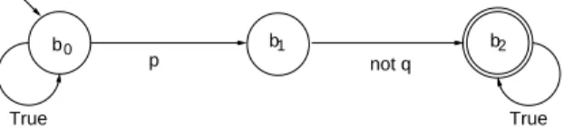
The automata encoding the properties 2(p ⇒ q), 2(p ⇒ ♦q) and 2(p ⇒ qUr) (represented in figures 3, 4 and 5) belong to the class BA2. We prove that
all the P LT L properties that can be encoded by an automaton of the class BA2
are modular properties.
Let P be a P LT L formula, and let σ be a path of a transition system T S such that σ ⊢ ¬P . Let σmbe the minimal suffix of σ that negates P , and let BA
be the B¨uchi automaton that encodes ¬P . We suppose BA ∈ BA2. Lemma 1
proves that a prefix of σmwhose all the states belong to the same module always
exists. Moreover, it proves that this prefix is at least two states long. Lemma 2 proves that when recognizing σm, BA can not get back to its initial state once it
has left it. In other words, we eliminate the loop on the initial state of BA (see figures 3, 4, 5). Theorem 3 concludes that if the above conditions are true, P is still negated on a module. It is obvious as BA is only composed of accepting states from the third one, and so the recognition will be “cut” on an accepting state. In other words, BA ∈ BA2 is a sufficient condition for P being a modular
property.
Lemma 1 Let P be a P LT L formula, σ a path of a transition system T S such that σ ⊢ ¬P , and σm= smsm+1. . . the minimal suffix of σ that negates P .
A prefix σ′
m of σm such that all the states in σ′m belong to the same module
always exists. The prefix σ′
m is at least 2 states long.
Proof. Consider the prefix only composed of the first two states of σm: σ′m =
smsm+1. smand sm+1belong to the same module. As a matter of fact, two cases
have to be considered:
1. sm and sm+1 belong to the same equivalence class. Then they basically
belong to the same module ;
2. smand sm+1belong to two distinct equivalence classes EQ and EQ′. Then
sm+1 is the target state of an outgoing transition of EQ and thus sm and
sm+1belong to the same module.
Lemma 2 Let P be a P LT L formula, σ a path of a transition system T S such that σ ⊢ ¬P , σm the minimal suffix of σ that negates P , and BA the B¨uchi
automaton that encodes ¬P .
σm= s0s1. . . is recognized by a path τ = b0b1. . . of BA where initial state
b0 only occurs once.
Proof. Let i > 0 be an integer such that bi= b0. Then, σi = sisi+1. . . is a suffix
of σ recognized by τi = bibi+1. . . . So, σi ⊢ ¬P , which is a contradiction since
Theorem 3 All the P LT L properties encoded by a B¨uchi automaton in the class BA2 are modular properties.
Proof. Let P be a P LT L formula, and let T S be a transition system which is split into a set M of modules. Let σ be a path of T S such that σ ⊢ ¬P , and σm = s0s1. . . be the minimal suffix of σ that negates P . Let finally BA =
< b0, B, AP, →BA, Accept > be a B¨uchi automaton such that BA ∈ BA2.
A prefix σ′
m= s0s1. . . sk of σmexists such that all the states involved in σm′
belong to a module M ∈ M. Moreover, σ′
m is at least 2 states long (lemma 1).
Let us prove that σ′
m⊢ ¬P .
We have σm ⊢ ¬P . So, a path τm = b0b1. . . of BA exists that recognizes
σm. Since BA ∈ BA2, we have: ∀i ≤ 2, bi ∈ Accept (lemma 2). Let us consider
the two following cases: – let σ′
m= s0s1. Then τm′ = b0b1b2 recognizes σ′mas b2∈ Accept
– let σ′
m = s0. . . sk with k > 1. Then τm′ = b0. . . bk+1 recognizes σ′m as
bk+1∈ Accept. As a consequence, σ′ m⊢ ¬P . Finally, T S 0 P ⇒ ∃M ∈ M ∧ σ′ mpath of M s.t. σ ′ m⊢ ¬P .
3.4 Modularity of the Three Modalities Introduced in B
In order to prove that 2(p ⇒ q), 2(p ⇒ 2q) and 2(p ⇒ qUr) are modular, we simply prove that the automatons of the negations of these patterns belong to BA2.
Pattern 1: 2(p ⇒ q) Suppose this property is false on the global graph. Then a path σ exists such that σ ⊢ ¬2(p ⇒ q) (which is equivalent to σ ⊢ ♦(p ∧ ¬q)). The B¨uchi automaton that encodes such a property is given in
b0 b1
True
b2
p not q
True
Fig. 3.B¨uchi automaton encoding ¬2(p ⇒ q)
Figure 3. It belongs to the BA2 class and thus 2(p ⇒ q) is modular.
Pattern 2: 2(p ⇒ ♦q) Suppose this property is false on the global graph. Then a path σ exists such that σ ⊢ ¬2(p ⇒ ♦q) (which is equivalent to σ ⊢ ♦(p ∧ 2¬q)). The B¨uchi automaton that encodes such a property is given in Figure 4. It belongs to BA2class and thus 2(p ⇒ ♦q) is modular.
b0 p and not q b1
True not q
Fig. 4.B¨uchi automaton encoding ¬2(p ⇒ ♦q)
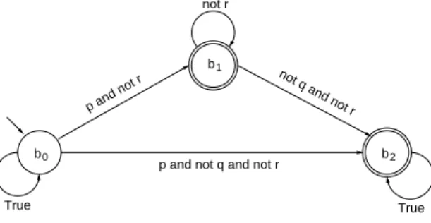
Pattern 3: 2(p ⇒ qUr) Suppose this property is false on the global graph. Then a path σ exists such that σ ⊢ ¬2(p ⇒ qUr) (which is equivalent to σ ⊢ ♦(p ∧ ¬(qUr))). The B¨uchi automaton which encodes such a property is
b0
not r
True True
b2 b1 not q and not r
p and not r
p and not q and not r
Fig. 5.B¨uchi automaton encoding ¬2(p ⇒ qUr)
given in Figure 5. It belongs to the class BA2 and therefore 2(p ⇒ qUr) is
modular.
4
Refinement and Modules
4.1 Modularity and Modules
Until now, we have only considered abstract partitions of the state space, without giving any indication on how to find a “good” partition. As a matter of fact, in order to prove in a modular way that a property P is true, P has to be true on every module. But with a random split of the transition system, it is possible that some modules find that P is false, whereas another split would have found P true on every module.
The question is, for a given modular property, how can we find a partition that makes the verification module by module successful ?
Our purpose here is to suggest a partition of the state space of a transition system into several components, this partition being based on a refinement re-lation. The refinement that we use is temporal in the sense that the system is observed more often. Thus, details such as new variables and new events are in-troduced step by step. They are observed between the old events in the abstract
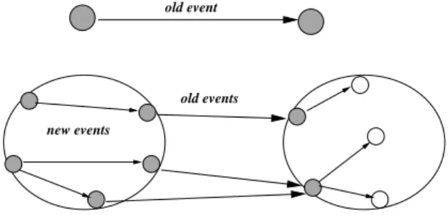
specification. The new properties are concerned with sequences of news events and it is suitable to verify them only on derived subsystems. We call old what is concerned with the abstract specification and new what is concerned with the refined specification.
old event
old events new events
Fig. 6.Refinement of an abstract transition
Let us recall some notions given in a paper published at IFM’99 [14]. Intu-itively, the figure 6 schematizes the refinement of an abstract transition t labeled with an old event into a family of refined transitions in which some conditions hold. We briefly define these notions informally.
– each labeled transition t is refined by a set of refined paths made of transi-tions labeled with the new events and terminated with a transition labeled by the label of t,
– the initial state of the abstract transition is refined by the initial states and all the intermediate states of the paths,
– the final state of the abstract transition is refined by the final states of all paths.
The modular verification of a P LT L property P consists in – computing the set of modules,
– verifying on each module by model-checking if P is satisfied or not, – concluding that P is satisfied if all the modules satisfy P .
In the rest of this section we explain why the modular verification concept concerns the modules of the refined specification, rather than the full specifica-tion. The introduced dynamic properties concern the new events in the modules obtained at this step from the abstract specification. Each module is described as a transition system obtained from a state by application of the new events. In the modules, the new states are pointed in and pointed out by the old events of the abstract specification. The new transitions are labeled by the new events. The verification of the dynamic properties is only performed on this state space augmented with its immediate neighbour states, on the border. Thus, semanti-cally, each old transition is refined by some chains of new events terminated by
a transition labeled by an old event. We establish the relation between a veri-fication on modules and a veriveri-fication on the whole system. In other words, we are essentially looking for conditions allowing us to perform local verifications rather than global ones.
4.2 B Events and Transitions Systems
We give some formal definitions for a B specification extended with P LT L for-mulae, and its semantics with a labeled transition system T S. The transition system semantics of a B specification is directly obtained from the Before/After predicate semantics of the B event systems given in [1], for the class of finite systems.
Modules are defined as particular labeled transition systems that refine a state and the set of transitions whose this state is source in the abstract speci-fication.
Definition 11 (Event System) An event system is a 6-tuple ES =< V, I, F, Init, A, GA> which consists of
– a set V of variables, – an invariant I, – a set F of formulae,
– an initial action Init to initialize variables, – an alphabet A of label of events,
– a set GA of events definitions in the shape select g then a end where g
denotes a proposition and a is a generalized substitution as defined in the B method [1].
Consider now two labeled transition systems T S1 =< A1, S1, S10, →1,
AP, L1 > and T S2 =< A2, S2, S20, →2, AP, L2 > semantics of ES1 =< V1, I1,
F1, Init1, A1, GA1 > and ES2=< V2, I2, F2, Init2, A2, GA2 >.
Definition 12 (Refinement of an Abstract Transition) A path σ2 of T S2
refines an abstract transition t = sto sa ′
∈→1 of T S1denoted σ2⊑ t iff
– σ2 = s1. . . sn is a finite path s.t. the transitions t1 = s0 a1
→ s1, . . . , tn−1 =
sn−2 an−1
→ sn−1 are labeled with new events
∀ti= si−1 ai
→ si∈→2 s.t. 1 ≤ i < n, ai∈ A/ 1∧ ai∈ A2 ,
– the label of the transition tn = sn−1 an
→ sn is the same than the one of t:
an = a,
– the valuations of all the states, except the last one, of the path σ2, do not
contradict the valuation of the source state of t
– the valuation of the final state of σ2 does not contradict the valuation of the
Definition 13 (Refinement of a Transition System) Let T S1 and T S2 be
two labeled transition systems. We define the set Σ of paths σ2 of LT S2 which
refine each abstract transition t ∈→1 enabled from s ∈ S1 as follows:
∀t = s→ sa ′
∈→1, ∀σ2= s0. . . sn path of T S2, σ2⊑ t ⇒ σ2∈ Σ .
Definition 14 (Module Derived from the Refinement) Let I2 be the
glu-ing invariant of ES2. A module of T S2, associated with a state s ∈ S1 and
an abstract transition t ∈→1 is a labeled transition system T S =< A, S, S0, →
, AP, L >where
– → is the set of transitions such that
∀σ2= t1. . . tn ∈ Σ, ∀i s.t. 1 ≤ i ≤ n, ti∈→ ,
– S is the set of states such that S = {s′ /s′ ∈ S2 and s ′ ∧ I2⇒ s}∪ {s′′ /∀t = si−1 ai → si∈→, s′′= si−1∨ s′′= si} ,
– S0 is the set of initial states such that
S0= {s′/s′∈ S ∧ ∀t = si−1 ai
→ si∈ T, s′6= si} .
Informally, a module is a labeled transition system defining all paths σ2 of
T S2 which refines each abstract transition t enabled from one state s ∈ S1.
Notice that the number of modules in T S2is the number of states in T S1.
The specification refinement guarantees essentially three points for a labeled transition system
– the refinement of each transition of the abstract transition system by a set of refined paths,
– the connectivity between the paths of the modules with the abstract transi-tions,
– the modules are free from deadlocks and livelocks.
All these definitions, and the consequences of the refinement of specification are established and proved in [5].
5
Specifications of the Robot Example
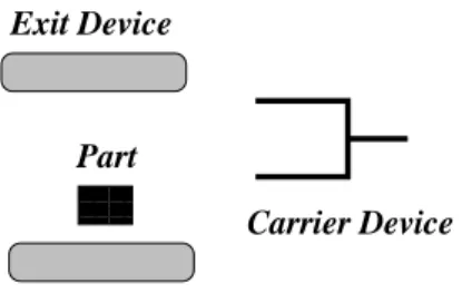
In order to make these notions clear, we illustrate them with the example of an industrial robot composed of an Arrival Device, an Exit Device and a Carrier Device. This robot carries some parts by moving from the Arrival Device to the Exit Device. We first give an abstract specification and then we give two refinement levels of the system. The indices 0, 1 and 2 of the variables indicate the level of refinement.
5.1 Informal Specification
The figure 7 represents the physical system. The Carrier Device (called CD) takes a part from the Arrival Device (called AD) and places it on the Exit Device (called ED). We first describe it as an abstract system, considering only two operations to load and unload a part. It simply consists in the Carrier Device taking a part and putting it onto the Exit Device.
00 00 00 00 11 11 11 11 Arrival Device Part Exit Device Carrier Device
Fig. 7.The robot
Informal Presentation of an Extended B Specification We describe a specification as an abstract system as in B[1]. It is composed of two parts.
– a descriptive specification that indicates what the system does, – an operational specification that indicates how the system proceeds.
The descriptive specification is essentially composed of a list of variables and of an invariant expressing safety properties restricting the set of valid states. In order to complete this part, we have proposed an extension of those systems with dynamic properties such as liveness, in the shape of P LT L formulae. In the example produced below, we use the four future temporal operators called usually Always, Next, Eventually and Until, denoted respectively by the symbols 2, , ♦ and U.
The operational specification is also composed of two parts. – the description of the initial states in the Initialization section,
– the description of all the events in the shape of guarded actions. The semantic of such an event is that it is enabled when the guard is true, and in that case the action is performed, so that it transforms the state of the system. The verification phase makes sure that both invariant and dynamic properties hold with the operational specification. As in the B method, the invariant is proved by means of a theorem-prover, but we will use a model-checker in order to verify the dynamic properties on the derived transition systems.
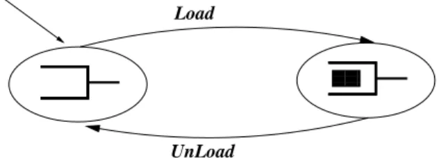
Abstract Specification In this first approach of the system, we focalize our observation on one component and we only look at the behaviour of the Carrier Device. We ignore what happens to the other devices. There are only two states: one when the device is free and one when it is busy. The specification proposed in figure 8 uses only one variable that gives the status of the Carrier Device denoted CD0 ∈ {f ree, busy}.The invariant property gives the sorting of the variables.
Two events are introduced in order to load and unload the part.
System Robot0
Variables V0={CDˆ 0}
Invariant I0=CDˆ 0∈ {f ree, busy}
Dynamic propertiesP01=2(CDˆ 0= busy ⇒ ♦CD0= f ree)
Initialization Init0=CDˆ 0:= f ree
Events Load0= Select CDˆ 0= f ree then CD0:= busy end
U nload0= Select CDˆ 0= busy then CD0:= f ree end
end Robot0
Fig. 8.Abstract specification of the robot
The dynamic property P01 is a liveness property that states that when the
Carrier Device is busy, then eventually it becomes free.
The corresponding transition system is represented in figure 9. It has two states and two events. It represents all the execution paths by means of a finite state system [3]. In this case, there is only one variable with two possible values. The transitions are labeled with the events Load and Unload representing the evolution of the system from one state to another.
000 000 000 000 111 111 111 111 Load UnLoad
Fig. 9.The abstract transition system
5.2 Refined Specification
Informal Presentation of a Refinement of Specification As in the B method [1], we use the concept of refinement. The idea is to enhance the detail level of observation of the system, so that the refined specification gives further details on what the system does and how it proceeds. Thus, refinement after refinement, the description will go from a high level specification to a specifi-cation that can be directly implemented. The refined specifispecifi-cation contains the same sections than the abstract one: Variables, Invariant, Dynamic Properties, Initialization and Events.
The figure 10 gives a refined specification of the Robot. Both abstract and refined specifications must respect the following constraints:
– the two sets of variables are disjoint,
– the new invariant, also called the gluing invariant, expresses a relation be-tween the two sets of variables of the two levels,
– the dynamic properties are new properties concerning the behaviour induced by the new events,
– the old events are described again in such a way that they are refined, – the new events are introduced.
In the B method, the refinement relation is verified and warrants the abstract invariant properties. The old dynamic properties are preserved by refinement notion as defined in [2]. This question is not treated in this paper in which we consider only the verification of new dynamic properties.
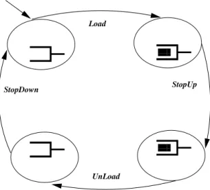
First Refinement of the Robot The refined specification in figure 10 settles the following point: the Carrier Device moves into two directions denoted U p and Down. The U p movement specifies that the Carrier Device is busy and goes up to the Exit Device in order to put a part. The Down movement specifies that it goes to the Arrival Device in order to take another part. We only need one new variable P osCD1∈ {Down, U p} which statues the position of the Carrier
Device.
The variables of the levels 0 and 1 are glued by the gluing invariant. The old events are refined with the new constraints and keep the same label. The guards of the events are reinforced. We have two new properties for this specification and they concern only the movement of the Carrier Device. They are safety properties. The properties P11 and P12 ensure that when the Carrier Device
goes up it is busy, and when it goes down it is free. The transition system associated to this first refinement of the specification is given in figure 11. Second Refinement of the Robot From this specification and with the same process, we give another refinement through a third detailed specification by introducing the component Exit Device. When a part is in it, it can be removed. Two news variables ED2 and AD2 are introduced with the possible values free
or busy. Once again, the old events are refined and the guards are reinforced. Two new events are introduced, denoted ArrivalP art2 and Evac2. The first
System Robot1 refines Robot0
Variables V1={CDˆ 1, P osCD1}
Invariant I1={CDˆ 1= CD0∧ P osCD1∈ {Down, U p}}
New Dynamic PropertiesP11=2(P osCDˆ 1= Down ∧ (P osCD1= U p)
⇒ CD1= busy)
P12=2(P osCDˆ 1= U p ∧ (P osCD1= Down)
⇒ CD1= f ree)
Initialization Init1=CDˆ 1 := f ree ∧ P osCD1:= Down
Old Events
Load1=ˆ Select CD1= f ree ∧ P osCD1= Down
then CD1:= busy end
U nload1=ˆ Select CD1= busy ∧ P osCD1= U p
then CD1:= f ree end
New Events
StopU p1=ˆ Select CD1= busy ∧ P osCD1= Down
then P osCD1:= U p end
StopDown1=ˆ Select CD1= f ree ∧ P osCD1= U p
then P osCD1:= Down end
End Robot1
Fig. 10.First refinement of the robot specification
000 000 111 111 000 000 111 111 Load StopDown StopUp UnLoad
transports it to the Exit Device. The second event removes the part from the Exit Device. The figure 12 gives the obtained specification.
System Robot2refines Robot1
Variables V2={CDˆ 2, P osCD2, AD2, ED2}
Invariant I2={CDˆ 2= CD1∧ P osCD2= P osCD1
∧AD2∈ {f ree, busy} ∧ ED2∈ {f ree, busy}}
New Dynamic propertiesP21=2(CDˆ 2= busy ⇒ CD2= busy
U (CD2= busy ∧ ED2= f ree))
Initialization Init2=CDˆ 2:= f ree ∧ P osCD2:= Down
Old Events
Load2=ˆ Select CD2= f ree ∧ P osCD2= Down
then CD2:= busy end
U nload2=ˆ Select CD2= busy ∧ P osCD2= U p
then CD2:= f ree end
StopU p2=ˆ select CD2 = busy ∧ P osCD2= Down
then P osCD2:= U p end
StopDown2=ˆ Select CD2= f ree ∧ P osCD2= U p
then P osCD2:= Down end
New Events
P artArrival2=ˆ Select AD2 = f ree then AD2:= busy end
Evac2=ˆ Select ED2= busy then ED2:= f ree end
End Robot2
Fig. 12.The second refinement specification
The gluing invariant states that the variables are identical to their abstrac-tion. The dynamic property P21 states that the Carrier Device remains busy
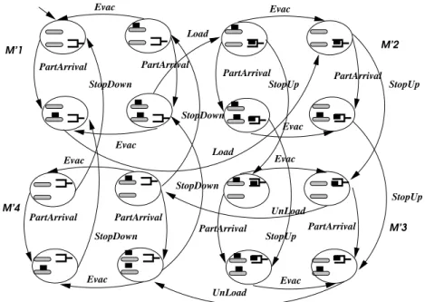
until the Exit Device is free. The labeled transition system given in figure 13 re-fines the labeled transition system of figure 11. It is divided into 4 modules. The modules M′
1 and M ′
3 both contain 6 states and 6 transitions, and the modules
M′ 2and M
′
4both contain 8 states and 8 transitions.
5.3 Verification of the Properties
We summarize the results of the modular verification of the properties P01,
P11, P12 and P21 presented above. These 4 dynamic properties have the B¨uchi
automata of their negations in BA2 and so they are modular properties. It is
sufficient that we verify them on each module in separation. They can be verified by a simple model-checking.
– P01=2(CDˆ 0 = busy ⇒ ♦CD0= f ree) is satisfied in the abstract
specifica-tion at the level 0.
– P11=2(P osCDˆ 1 = Down ∧ (P osCD1 = U p) ⇒ CD1 = busy) from
PartArrival PartArrival Evac Evac PartArrival PartArrival Evac UnLoad UnLoad Evac Evac Evac PartArrival StopDown StopDown StopUp StopUp StopDown StopDown PartArrival Evac Evac Load M’3 M’2 M’1 M’4 Load StopUp StopUp PartArrival PartArrival
Fig. 13.The second refined transition system
that P osCD1 = Down and there is no successor. We then conclude that
P osCD1= Down ∧ (P osCD1= U p) is false and globally P11 is satisfied.
– P12=2(P osCDˆ 1 = U p ∧ (P osCD1= Down) ⇒ CD1= f ree) from level
1 is satisfied in M1. We use the same reasoning than P11.
– P21=2(CDˆ 2= busy ⇒ CD2= busyU(CD2= busy ∧ ED2= f ree)) defined
on level 2 is satisfied modularly on M′
2 and on M ′
3. In the other modules
M′ 1and M
′
2we have 2(CD2= f ree). We then conclude that P21 is globally
satisfied.
6
Conclusion
We propose a technique that allows the modular verification of a class of usual dynamic properties of reactive systems. These properties are safety and liveness properties, and they are checked by means of a model-checker. The main problem in applying this technique based on reachability analysis is the potential combi-natorial explosion of the state space. In order to attack this problem, we define a strategy based on local verifications which uses the refinement process. From the abstract specification of a B event system, we derive a detailed specification by introducing news events. We then look at the new properties that have to be checked on the chains of new events. These properties are verified on modules rather than on the whole transition system, and consequently the verification of a P LT L property reduces to the verification of a local P LT L property.
For some specific dynamic property patterns, we have exhibited sufficient conditions to assert that if a P LT L property is satisfied on each module, then it is globally satisfied. The negations of these modular properties are recognized by particular B¨uchi automata that we describe. However, in some cases, if the verification of the property fails on a module, we cannot conclude about the satisfaction of this property. This situation is possibly due to the fact that the property should have been established at an abstract level of abstraction because it uses a chain of old events. This point has already been discussed and published at the Conference IFM’99 in York [14].
We have shown in [19] another possibility to reduce the complexity of ver-ification by model-checking for large systems which consists of a combination of model-checking and theorem-proving techniques. Patterns in the shape of 2(p ⇒ Q) can be studied in two verifications. Invariance properties 2¬p can be verified with the prover and temporal properties ♦p ∧ 2(p ⇒ Q) with a model-checker. Then, there are two kinds of modules: those in which we have 2¬p and those in which some states verify p. In the first case, the B prover is the proper tool for proving2¬p. Thus, the modules are treated separately without commu-nication. In practice, we are working at the implementation of a verification tool using both the B and SPIN environments.
The work that we present in this paper only uses the syntactic way to char-acterize the modular dynamic properties, without taking into account their se-mantics. The modular class is formed of patterns in the shape of 2(p ⇒ Q), where p is a proposition and Q is a temporal formula such as q, ♦q, and qUr. We project in future research to extend this class of properties by using the semantics level of the specification. We know that a module is exited with tran-sitions that correspond to the occurrence of old events. The idea is to use this information in order to prove that some properties (not in BA2) are modular in
the very context of such a semantic modular split. This class of P LT L properties could combine many different temporal operators.
References
1. J.-R. Abrial. The B Book : Assigning Programs to Meanings. ISBN 0521-496195. Cambridge University Press, 1996.
2. J. R. Abrial and L. Mussat. Introducing dynamic constraints in b. In Second Conference on the B method, France, LNCS 1393, pages 83–128. Springer Verlag, April 1998.
3. A. Arnold. Syst`emes de transitions finis et s´emantique des processus communicants. Masson, 1992.
4. A. Arnold and S. Brlek. Automatic verification of properties in transition systems. Software-Practice and Experience, 25(6):579–596, 1995.
5. F. Bellegarde, J. Julliand, and O. Kouchnarenko. Ready-simulation is not ready to express a modular refinement relation. In Proc. Int. Conf. on Fondamental Aspects of Software Engineering, FASE’2000, volume 1783 of Lecture Notes in Computer Science, pages 266–283. Springer-Verlag, April 2000.
6. C. Courcoubetis, M. Vardi, P. Wolper, and M. Yannakakis. Memory efficient al-gorithms for the verification of temporal properties. Formal Methods in System Design, 1:275–288, 1992.
7. Cu´ellar, I. Wildgruber, and D. Barnard. Combining the design of industrial systems with effective verification techniques. In FME’94, LNCS n. 873, pages 639–658. Springer Verlag, 1994.
8. P. Godefroid. Partial-order methods for the verification of concurrent systems. LNCS, 1032, 1996.
9. P. Godefroid and G.-J. Holzmann. On the verification of temporal properties. In PSTV’93, June 1993.
10. G.-J. Holzmann. Design and validation of computer protocols. 1991.
11. G.-J. Holzmann. The model checker spin. In IEEE Trans. On Software Engineer-ing, volume 23, 1996.
12. G.-J. Holzmann. State compression in spin. In 3rd
SPIN Workshop, Twente University, April 1997.
13. H. Hungar. Combining model checking and theorem proving to verify parallel processes. In C. Courcoubetis, editor, 5th International Conference on Computer Aided Verification: CAV’93, number 697 in LNCS, Elounda, June/July 1993. 14. J. Julliand, P.A. Masson, and H. Mountassir. Modular verification of dynamic
properties for reactive systems. In International Workshop on Integrated Formal Methods (IFM’99), pages 89–108, York, UK, June 1999. Springer Verlag.
15. K. Laster and O. Grumberg. Modular model-checking of software. In TACAS’98, Lisbon, March-April 1998.
16. Z. Manna and A. Pnuelli. The Temporal Logic of Reactive and Concurrent Systems: Specification. ISBN 0-387-97664-7. Springer-Verlag, 1992.
17. Z. Manna and A. Pnuelli. Temporal verification of reactive systems. ISBN 0-387-94459-1. Springer Verlag, 1995.
18. R. Milner. Communication and Concurrency. Computer Science. Prentice-Hall, 1989.
19. H. Mountassir, F. Bellegarde, J. Julliand, and P.A. Masson. Coop´eration en-tre preuve et model-checking pour v´erifier des propri´et´es LTL. In congr`es AFADL’2000, Grenoble, December 2000.
20. D. Peled and W. Penczeh. Using asynchronous b¨uchi automata for efficient verifi-cation of concurrent systems. In Symposium on Protocol Specifiverifi-cation Testing and Verification, pages 90–100, Warsaw, Pologne, June 1995.
21. D. A. Peled. Combining partial order reduction with on-the-fly model-checking. In CAV’94, LNCS n. 818, pages 377–390. Springer Verlag, June 1994.