HAL Id: hal-02612369
https://hal.archives-ouvertes.fr/hal-02612369v2
Submitted on 4 Jun 2020
HAL is a multi-disciplinary open access
archive for the deposit and dissemination of
sci-entific research documents, whether they are
pub-lished or not. The documents may come from
teaching and research institutions in France or
abroad, or from public or private research centers.
L’archive ouverte pluridisciplinaire HAL, est
destinée au dépôt et à la diffusion de documents
scientifiques de niveau recherche, publiés ou non,
émanant des établissements d’enseignement et de
recherche français ou étrangers, des laboratoires
publics ou privés.
Approximate Buffers for Reducing Memory
Requirements: Case study on SKA
Hugo Miomandre, Jean-François Nezan, Daniel Menard, Adam Campbell,
Anthony Griffin, Seth Hall, Andrew Ensor
To cite this version:
Hugo Miomandre, Jean-François Nezan, Daniel Menard, Adam Campbell, Anthony Griffin, et
al..
Approximate Buffers for Reducing Memory Requirements: Case study on SKA. 34th 2020
IEEE Workshop on Signal Processing Systems (SiPS), Oct 2020, Coimbra, Portugal. pp.9195262,
�10.1109/SiPS50750.2020.9195262�. �hal-02612369v2�
Approximate Buffers for Reducing Memory
Requirements: Case study on SKA
Hugo Miomandre
∗, Jean-Franc¸ois Nezan
∗, Daniel Menard
∗, Adam Campbell
†, Anthony Griffin
†,
Seth Hall
†and Andrew Ensor
†∗ INSA Rennes, UMR CNRS IETR, Rennes, France
†High Performance Computing Research Laboratory, AUT, Auckland, New-Zealand
Abstract—The memory requirements of digital signal process-ing and multimedia applications have grown steadily over the last several decades. From embedded systems to supercomputers, the design of computing platforms involves a balance between processing elements and memory sizes to avoid the memory wall. This paper presents an algorithm based on both dataflow and approximate computing approaches in order to find a good balance between the memory requirements of an application and the quality of the result. The designer of the computing system can use these evaluations early in the design process to make hardware and software design decisions. The proposed method does not require any modification in the algorithm’s computations, but optimizes how data are fetched from and written to memory. We show in this paper how the proposed algorithm saves 23.4% of memory for the full SKA SDP signal processing computing pipeline, and up to 68.75% for a wavelet transform in embedded systems.
Index Terms—Signal Processing, Radio Astronomy, SKA Project, Approximate Computing, Dataflow Models
I. INTRODUCTION
Memory issues strongly impact the quality and performance of computing systems. The area occupied by the memory can be as large as 80% of a chip and may be responsible for a major part of the power consumption of both Edge Computing [1], [2] and High-Performance Computing (HPC) systems [3]. As new digital signal processing and multimedia applications require more and more data to process and store, processing elements, internal memories and external storage components increase in number and size. Computing systems are growing more heterogeneous and interconnects more com-plex in order to increase computational performance while keeping energy consumption under control. Solving memory issues remains a challenging objective in both Edge and HPC Computing systems.
The worlds largest radio telescope project, the Square Kilo-metre Array (SKA), will have to generate real-time multidi-mensional images of the sky from a 7.2 Terabit/s data stream without the option of storing the raw input data. The SKA Science Data Processor (SDP) computing system will be a dedicated low-power HPC architecture combining a mixture of primary processors and hardware accelerators to achieve its exascale computing requirements at low power within the next decade. The SDP computing system has to be designed and sized taking into account unprecedented data throughput requirements, constrained budget, computing precision and energy efficiency. The memory architecture of the SDP must
be accurately evaluated so as suitably balance these concerns. The need for methods and tools to accurately evaluate the exascale memory requirements of SKA is the initial motivation of the work presented here.
Dataflow graphs are often used to model, analyse, map and schedule concurrent digital signal processing and multimedia applications. Most of the work done in this area has been applied to the design of embedded systems, but methods and tools based on dataflow graphs are now also studied in the con-text of SKA exascale computing [4], [5]. Dataflow MoC allows the specification of applications in the form of graphs whose nodes, called actors, are the functions executed, and whose arcs are First-In First-Out queue (FIFO) buffers ensuring data transfers between the actors. Most of the literature on dataflow models focuses on the optimisation of timing performance, such as execution rate or throughput, or the computation of the minimal number of FIFO buffers to implement a static periodic schedule [6]. Optimizing buffer sizes is usually done by decreasing the number of tokens in each buffer [7], [8]. In [9], the dataflow graph is used to compute memory bound requirements of an application. In [10], the amount of allocated memory is minimized by memory reuse: the buffer lifespan is calculated depending on the actor scheduling and the analysis of lifespans enables several buffers to share the same memory space at run-time, reducing the required global memory space. In this paper, we present a complementary size-reduction method that can be used in addition to previous dataflow memory optimizations. Our method uses the Approximate Computing (AxC) paradigm [11] to define the minimal binary representation of the tokens in FIFO buffers, taking into
consideration both computational accuracy and complexity. The goal is to decrease both the memory footprint and the energy consumption of the application without signficantly reducing the quality of output.
The proposed method has been evaluated on two use cases: an implementation of the SKA imaging pipeline illustrating exascale signal processing on HPC systems, and a wavelet transform illustrating generic image processing on embedded systems.
Section II provides the context of the study and the related background concepts on dataflow models and approximate computing used in this paper. Section III details the concept of Approximate Buffer introduced in this paper. Finally, Sec-tion IV presents the experimental evaluaSec-tion of the
Approxi-Configuration port Parameter Parameter dependency Initial tokens FIFO Actor
A
Data port and rate 1 x4 P(a) PiSDF Model of Computation (MoC) semantics
Read
frame
DWT
IDWT
Display
frame
H
W
N
NbSlice
Setter
(b) PiSDF graph of an image filtering application
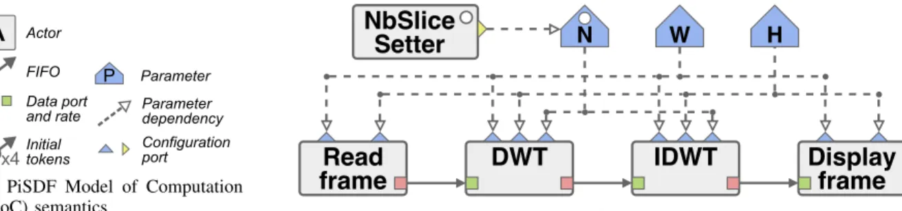
Fig. 1: Parameterized and Interfaced Synchronous Dataflow (PiSDF) MoC semantics and example mate Buffer technique and Section V concludes this paper.
II. CONTEXT ANDBACKGROUND
A. PiSDF MoC
The reconfigurable dataflow MoC studied in this paper is the Parameterized and Interfaced Synchronous Dataflow (PiSDF) MoC [12]. Fig. 1 depicts the graphical elements of the PiSDF semantics and gives the example of a graph, composed of four actors, implementing a Discrete Wavelet Transform (DWT) and an Inverse Discrete Wavelet Transform (IDWT) applied to each frame of a video sequence. In this example, the resolution of the video is set by the W and H parameters which are nodes specifying the width and the height of each frame of the video sequence. Production and consumption rates of actors are specified with numerical values or expressions depending on parameters. Rate configuration parameters are used to specify application reconfigurations in the PiSDF MoC. Following PiSDF execution rules [12], an actor may trigger a reconfiguration of the graph topology and intrinsic parallelism by setting a new parameter value at runtime.
At each iteration of the graph, corresponding to the pro-cessing of a new frame, the NbSliceSetter actor triggers a reconfiguration of the data rates by assigning a new value to parameter N . Reconfigurations enable a dynamic variation of the number of parallel executions of actors inside DWT and IDWT subgraphs. The parameter N is used internally by these subgraphs to parallelize inner 1D-convolutions actors by splitting the processed frame into slices.
B. Square Kilometre Array Dataflow Model
The SKA1 project aims to build the world’s largest radio telescope, with eventually over a square kilometre of effective collecting area. It will consist of hundreds of thousands of antennas and hundreds of dishes. The collected data are fed to the Central Signal Processor (CSP) on site which handles front-end processing before sending it across dedicated long haul fibre links to the SDPs, which converts it into data and images suitable for radio astronomers.
The SDP Imaging Pipeline2 is an implementation of the
SKA SDP for its most compute intensive task. It produces images from visibility data output from the CSP. It is this
1https://www.skatelescope.org/
2https://gitlab.com/ska-telescope/sep pipeline imaging/
Gains Gridding Apply Deconvolution DFT Gains Calib Output Image From CSP
Fig. 2: Simplified representation of the SEP.
implementation of the SKA SDP that has been chosen as a use case in this paper. The SDP Imaging Pipeline generates sky images with an iterative process, refining the image on every major cycle. Each of these major cycles goes through a deconvolution step, tasks with extracting relevant “bright” sources during each of its minor cycles. In this paper, the dataset we have been using has been generated from a GLEAM observation3 in order to generate sky images we can
analyse in terms of quality. The dataset used is generated for a 15 minute observation with a visibility per baseline each 30 seconds for 512 antennas. In comparisons SKA will have hundreds of receivers producing billions of visibilities per second.
The SDP Imaging Pipeline has been represented for the first time as a PiSDF graph using PREESM4. The complexity to represent an algorithm like the SDP Imaging Pipeline lies in the fact that the algorithm is iterative. Fig. 2 shows a simplified representation. The delay between the actors Gains Calib and Gains Applyis used to represent the major cycles of the SDP Imaging Pipeline and the delay on the actor Deconvolution is used to represent the minor cycles. The PiSDF graph of the SDP is made up of 150 actors and 280 FIFObuffers. This graph is then flattened by PREESM in a Single-rate Directed Acyclic Graph (SrDAG) for the analysis, the mapping-scheduling and the code generation steps. The SrDAG of the SDP is made up of 4430 actors and 11850 FIFO buffers using the parameters of the GLEAM dataset we used.
C. Approximate Computing
Several approaches have been proposed as AxC to decrease the computation complexity, the memory footprint and the energy consumption of an application. AxC techniques can be divided into three categories : Computation Level AxC, Hardware Level AxC and Data Level AxC. Data Level AxC
3http://www.mwatelescope.org/gleam-x 4https://github.com/preesm/preesm/
techniques benefit from a reduction in either the amount of data to process (Data Reduction), or its actual representation in computer memory (Precision Optimization). The contribution of this paper is related to Data Level Precision Optimization AxC techniques.
The Precision Optimization process requires modifications that impact an algorithm at its core. Algorithms are first evalu-ated with the intent of producing high-accuracy results, usually using double-precision floating-point arithmetic and high-level programming languages (C/C++, Matlab, Python, ...). Such naive but straight-forward implementations come with high memory footprints, high compute processing requirements and poor timing performance. Their reference algorithms are then rewritten for specific embedded systems or exascale HPC systems to meet real-time and power consumption constraints. Considering the digital representation of data provides one avenue to meet these requirements at the expense of affecting the output accuracy [13].
Floating-point arithmetic is commonly used in application development for its ease of use. It offers both a high dynamic range and a high precision, and any necessary conversion step is handled directly by the hardware. According to the IEEE-754 standard [14], floating-point number representation is composed of three parameters: the exponent, the mantissa and the sign. The corresponding value is encoded as follow:
x = (−1)s× m × 2e
(1) where s is the sign bit, m the M-bit mantissa and e the E-bit exponent stored as an integer representing the position of the radix-point. The two most commonly used floating-point data-types are single precision floating-point and double pre-cision floating-point. Single prepre-cision floating-point numbers are 32-bit numbers represented with M = 24 and E = 8. Double precision floating-point numbers are 64-bit numbers represented with M = 53 and E = 11.
The penalty for using floating-points types over integers with basic operations such as addition and multiplication was evaluated in [15]. Compared with an integer adder, a floating-point adder requires an area 3.5 to 3.9 times larger, a power consumption between 12 and 15.7 times higher and latency around 2 times longer. Concerning the multiplication, a floating-point multiplier requires approximately 30% less area than an integer multiplier, has a similar latency, but has a power consumption up to 35 times higher.
Custom floating-point data types have found use in specific applications. For instance, the Posit arithmetic (also called Type III Unums) claims to have a larger dynamic range and a higher accuracy [16] than with IEEE-754 floating-point arithmetic. Posit arithmetic has been used successfully in areas including machine learning or graphics rendering but not in ar-eas such as particle physics simulations [17]. Another example of alternative data types is the 16-bit half-precision floating-point format is defined in the IEEE 754-2008 standard [14]. The internal architectures, instruction sets and compilers of Central Processing Units (CPUs), Digital Signal Processors (DSPs) and Graphics Processing Units (GPUs) have to be
optimised for the management of new data types. Otherwise their use implies specific implementations on Application-Specific Integrated Circuits (ASICs) or Field-Programmable Gate Arrays (FPGAs). A specific and time consuming study is thus required to ensure the benefits and the validity of results in a targeted application using standard or custom data-types. Another way to satisfy implementation or real-time con-straints is the use of fixed-point arithmetic representing floating-point values as integers. A number x is encoded using fixed-point arithmetic with three parameters, the sign-bit s, the number of bits m used to encode the integer part, and the number of bits n used to encode the fractional part. The sum m + n + 1 gives the total width of the data. m represents the distance in number of bits between the radix-point and the Most Significant Bit (MSB) and n the distance between the radix-point and the Least Significant Bit (LSB). The fixed-point representation xF xP of the floating-point number x is
obtained as:
xF xP = < x × 2n> × 2−n (2)
with < . . . > being the rounding mode. The data is encoded as follow: xF xP = −2m× S + m−1 X i=−n bi× 2i (3)
where bi is the value of bit i. Fixed-point arithmetic is
more complicated to use than floating-point as it requires determining the suitable parameters m and n for each variable. It also has a lower dynamic range. However, the position of the radix-point is known at compile-time in fixed-point arithmetic, not stored with the exponent field as done in floating-point arithmetic, allowing hardware and software op-timizations. Fixed-point DSPs are cheaper than their floating-point counterparts, and fixed-floating-point implementation are faster on General Purpose Processors (GPPs).
III. APPROXIMATEBUFFER
Evaluating the relative merits of different representations is time consuming and require specific knowledge in both hardware and software domains. Our contribution detailed in this section is the application of AxC Precision Optimization techniques with the design approach based on dataflow models to automate and accelerate these evaluations. The idea behind the Approximate Buffer contribution is to store the data associated to edges of the PiSDF dataflow graph in FIFO
buffers using fewer bits than what would be expected by the data-type used during computations inside the nodes of the graph.
In the dataflow approach, the processed data are of two types : the data associated with actors (nodes of the graph) and the data associated with the FIFO buffers (edges of the graph). As the code inside actors is imperative code, the use of usual AxC Precision Optimization is possible but requires a fine knowledge of the algorithm and modifications inside the imperative code. In our approach, we evaluate the impact of AxC Precision Optimization on data associated with FIFObuffers without any modification of the imperative code,
32 32 32 32 32 32 32 32
Original memory footprint
20 20 20 20 20 20 20 20 96
Reduced memory footprint Saved space
Working Size
Storage Size
Fig. 3: Variable data-width buffer, from 32 down-to 20 bits. enabling a controlled degradation of the output quality at the price of a small performance penalty.
A. Variable data-width
As mentioned in Section II-C, algorithms are usually de-signed using 64-bit double-precision or 32-bit single-precision floating-point arithmetic, as these data representations enable the use and computation of non-integer numbers. However, this available precision can often be underused. Regardless of how much precision is required for a floating-point variable, it still occupies the same memory space. The same applies to integer variables. Standard data-types sizes tend to occupy either 8, 16, 32, 64 or 128 memory bits.
Depending of the nature of the data, a number N of bits, either LSB or MSB, could be scrapped to reduce the size of the data-type associated to a FIFObuffer, and thus of the whole buffer. Fig. 3 shows a simplified representation of this.
Without any intermediate representation of the data stored in an Approximate Buffer, whether to discard some LSBs and/or MSBs depends on the initial data representation.With floating-point variables, discarding LSBs means removing lower bits from the mantissa. How many bits can be removed from the mantissa is bounded by the acceptable degradation of the output quality, as well as the actual size of the mantissa itself. For integer data-types, similarly to floating-point data-types, removing LSBs leads to an increasing degradation of the output quality. However, if values in the array do not reach the 2N threshold, then it becomes possible to remove M − N MSBs without any loss in terms of output quality for data represented by M bits.
One of the objectives of this method is to be as least intrusive as possible with modifications to the orig-inal algorithm. Indeed, while methods such as fixed-point arithmetic would require the algorithm to be widely re-designed, our method only requires modifying data ac-cess schemes. In case of a C-like syntax, the data-writing process would be modified from array[index] = value; to ApproxFifoSet(&ApxFifo, index, value);. To correctly handle data insertions and extractions from the Approximate Buffer, a WorkingSize field and a StorageSizefield are kept as buffer metadata. They respectively correspond to the size of the datum in bits during processing and to the size of the datum in bits when stored in the array. This allows data stored on a reduced number of bits to be extracted and processed as originally intended, then stored back into a buffer. Future work will be to automatically
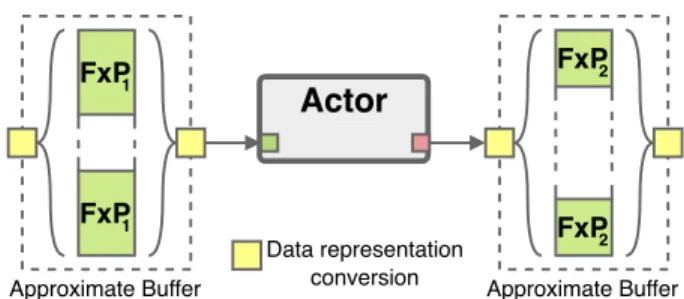
FxP2 FxP2
Actor
Approximate Buffer Data representation conversion Approximate Buffer FxP1 FxP1Fig. 4: Variable data-width buffer with FxP representation. generate the data access schemes defined here in PREESM to automate the process.
B. Custom data representation
As briefly mentioned in Section III-A, the original data representation in memory greatly affects the number of bits that can be removed. For example, using 32-bits floating-point variables, the actual value is encoded in the 23 LSBs, the rest serving as a scaling factor or the sign bit. This means the data-width reduction possibilities are limited.
To counter this issue, the chosen solution is to use an alternative data representation when storing inside the Ap-proximate Buffer. The alternate representation considered is the point format. As explained in Section II-C, fixed-point variables are presumed to have their exponent values known at compile time, meaning the order of magnitude of variables stored in the Approximate Buffer should be known beforehand. Unfortunately this may not be known in practice. To bypass this issue, the same exponent value is used for every data inside the Approximate Buffer. This common exponent value is stored as metadata for the Approximate Buffer, alongside the WorkingSize field and the StorageSize field. This allows floating-point variables to be stored in even fewer bits than the method described in Section III-A. A simple working example is shown in Fig. 4. F xP1 and F xP2 are two
fixed-point based data representation using different data-width. Data stored using the F xP1 representation are extracted
from the Approximate Buffer, converted into F P 32, which is the working datatype of this example, processed by Actor, then written into another Approximate Buffer using the F xP2
representation. As shown in Fig. 4, F xP1 and F xP2 can be
different formats using different numbers of bits.
In order to setup an appropriate common exponent value for the Approximate Buffer, two choices are available. The first consists in determining the maximum value that needs to be stored in the buffer. This can easily be done with an image processing pipeline, as pixels composing an image have bounded values. These values will vary in a predictable way depending on what image processing operations are applied. However, this might not be possible with an application processing unpredictable data. In the second approach, if the exponent value needed to store the data is higher than the current exponent value of the buffer, then the whole buffer can be re-evaluated to fit this new exponent. While this means that the previously stored data will lose some precision, it enables storing values that would otherwise end
20 40 60 80 100 120 0 50 100 150 200 250 PSNR value Memory footprint (MB) FP32 Reference Variable data-width
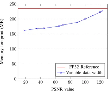
Fig. 5: PSNR dependant of SDP Imaging Pipeline Memory footprint
up overflowing. The main drawback of this storage method is that Approximate Buffers containing variables across a wide range might have their smallest values rounded to zero, which might be problematic with some applications. This issue may be solvable by using a custom floating-point representation. This approach will be investigated in future work.
IV. RESULTS
The proposed method was applied to two use cases to demonstrate its relevance as well as its drawbacks. It shows the possible gains in terms of memory footprint with the associated impact on output quality.
A. Results for the SDP Imaging Pipeline
The SDP Imaging Pipeline is an iterative process which in each major cycle produces a dirty image, containing interfer-ometry artifacts, and cleans it with a series of minor cycles that detect sources and remove them from the image. In this use-case, the first major cycle is a calibration cycle used to correct antenna gains, followed by imaging cycles to detect fainter and fainter sources. A total of 4 cycles are processed, producing an residualdirty image each time in which fainter sources can be resolved. The reference used for output quality measurements are the four dirty images produced by taking the precise but computationally-expensive direct Fourier Transform. From the PiSDF representation of the SDP, the peak memory usage is measured to determine an optimal buffer allocation. The size reduction methods described in Section III are then applied progressively on these buffers and the corresponding memory consumption and output quality degradation are measured and displayed in Fig. 5. The Peak Signal-to-Noise Ratio (PSNR) values displayed are the worst results obtained by comparing the reference dirty image of the Nthiteration with the corresponding dirty image obtained with reduced precision. The memory footprint of the base version of the SDP is 235 MB. It can be reduced to 223 MB (-5.1%) with a PSNR of
120dB down to 180 MB (-23.4%) while keeping a PSNR value of 70dB. From this point, reducing data precision any further prevents the SDP Imaging Pipeline from correctly finding the expected number of sky sources, leading to the generation of erroneous intermediate dirty images, hence the precision dip. As the SDP Imaging Pipeline is a complex application, it is not possible to precisely predict the extent of the quality degradation that comes with the use of Approximate Buffers. Reducing data-storage accuracy of one buffer can lead to a significant decrease in the output quality, but applying the reduction to a second one can, in some case, almost completely negate this degradation. Fine tuning the data-width in complex applications can be a lengthy but necessary process. This method leads to a performance penalty between 10 and 13% in this application, depending of how many buffers are impacted. This use case represents only a fraction of what the SKA SDP aspires to be. As stated in I and II-B, the SKA SDP pipeline will be designed to process multiple Terabit/s in real time. This tremendous amount of data to process will be scattered across compute nodes and is identified as one of its significant compute challenges.
B. Results for the Wavelet algorithm
The second use-case is an image processing pipeline con-sisting of a 2D-DWT followed by an 2D-IDWT, as shown in a simplified way in Fig. 1b. The goal of this example is to show that image processing algorithms can be very resilient to precision reduction, and not just in terms of subjective perception, and that memory footprint reduction methods shown in this paper are not limited to applications such as SKA.
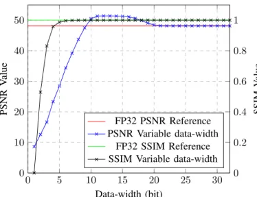
This experiment applies the DWT to a video stream, stores the result in Approximate Buffers, then applies the IDWT. The output degradation compared to an unprocessed reference is shown in Fig. 6, and compared to a FP32 result in Fig. 7. The metrics used to evaluate quality are the PSNR and the Structural SIMilarity (SSIM).
It shows that the data-width can be reduced from the original 32 bits of single precision floating-point representation down to 10 bits without too much degradation, a 68.75% size reduction. In fact, in this example, the output images obtained by using a data-width from 22 bits and up shows the PSNR beyond 100 dB, and are strictly identical to the output of the reference FP32 version for data-width ranging from 29 to 32 bits.
Interestingly enough, according to Fig. 6, it appears that in some cases such as this one, reducing the precision can lead to better global output quality. The output image obtained by reducing data-width from 32 down to 10-to-19 bits is closer to the original image than the output obtained using the reference FP32 data representation, with a PSNR value above 48.1dB.
V. CONCLUSION
This paper presents a new AxC technique oriented not toward reducing the computation intensity of an application but rather reducing its memory footprint. It stores data encoded
0 10 20 30 40 50 PSNR V alue 0 5 10 15 20 25 30 0 0.2 0.4 0.6 0.8 1 Data-width (bit) SSIM V alue FP32 PSNR Reference PSNR Variable data-width FP32 SSIM Reference SSIM Variable data-width
Fig. 6: PSNR and SSIM dependant of buffer data-width on the Wavelet application compared to unprocessed image (Fig.1b)
0 50 100 150 PSNR V alue 0 5 10 15 20 25 30 0 0.2 0.4 0.6 0.8 1 Data-width (bit) SSIM V alue PSNR Variable data-width SSIM Variable data-width
Fig. 7: PSNR and SSIM dependant of buffer data-width on the Wavelet application compared to FP32 (Fig.1b)
with a variable number of bits into buffer, while allowing the use of alternative data representations to mitigate the loss of precision.
We have shown the relevance of these methods in ap-plications such as the SDP Imaging Pipeline, an important component of the SKA processing, as well as in a classic image processing algorithm. It displays promising results in both memory footprint reduction and output quality tolerances. An interest of our work is to enable memory-constraint architectures to process algorithms which previously had too large a memory footprint. Another interest is also to improve performance on parallel architectures bounded by their mem-ory or interconnect bandwidth, such as multi-core embedded systems, multi-node HPC systems or hardware accelerators.
The proposed method will first be extended to the use of custom floating-point representations to mitigate the output quality degradation even further and increase memory savings.
As our method only requires the modification of data access schemes in the code associated with PiSDF FIFO buffers, future work will be to extend and integrate the proposed AxC technique in PREESM to provide a solution without any user code modification.
REFERENCES
[1] E. de Greef, F. Catthoor, and H. de Man, “Array placement for storage size reduction in embedded multimedia systems,” in Proceedings of the IEEE International Conference on Application-Specific Systems, Architectures and Processors, ASAP 97, (USA), p. 66, IEEE Computer Society, 1997.
[2] W. A. Wulf and S. A. McKee, “Hitting the memory wall: Implications of the obvious,” SIGARCH Comput. Archit. News, vol. 23, p. 2024, Mar. 1995.
[3] D. Zivanovic, M. Pavlovic, M. Radulovic, H. Shin, J. Son, S. A. Mckee, P. M. Carpenter, P. Radojkovi´c, and E. Ayguad´e, “Main memory in hpc: Do we need more or could we live with less?,” ACM Transactions on Architecture and Code Optimization (TACO), vol. 14, no. 1, pp. 1–26, 2017.
[4] Dask Development Team, Dask: Library for dynamic task scheduling, 2016.
[5] C. Wu, R. Tobar, K. Vinsen, A. Wicenec, D. Pallot, B. Lao, R. Wang, T. An, M. Boulton, I. Cooper, R. Dodson, M. Dolensky, Y. Mei, and F. Wang, “Daliuge: A graph execution framework for harnessing the astronomical data deluge,” CoRR, vol. abs/1702.07617, 2017. [6] P. K. Murthy and S. S. Bhattacharyya, “Shared memory
implementa-tions of synchronous dataflow specificaimplementa-tions,” in Proceedings Design, Automation and Test in Europe Conference and Exhibition 2000 (Cat. No. PR00537), pp. 404–410, 2000.
[7] O. Moreira, T. Basten, M. Geilen, and S. Stuijk, “Buffer sizing for rate-optimal single-rate data-flow scheduling revisited,” IEEE Transactions on Computers, vol. 59, no. 2, pp. 188–201, 2010.
[8] A. Bouakaz, P. Fradet, and A. Girault, “Symbolic buffer sizing for throughput-optimal scheduling of dataflow graphs,” in 2016 IEEE Real-Time and Embedded Technology and Applications Symposium (RTAS), pp. 1–10, 2016.
[9] K. Desnos, M. Pelcat, J. F. Nezan, and S. Aridhi, “Memory Bounds for the Distributed Execution of a Hierarchical Synchronous Data-Flow Graph,” in 12th International Conference on Embedded Computer Systems: Architecture, Modeling and Simulation (SAMOS XII), (Agios Konstantinos, Greece), p. 160, July 2012.
[10] K. Desnos, M. Pelcat, J. F. Nezan, and S. Aridhi, “On Memory Reuse Between Inputs and Outputs of Dataflow Actors,” ACM Transactions on Embedded Computing Systems (TECS), vol. 15, p. 30, Feb. 2016. [11] A. Agrawal, J. Choi, K. Gopalakrishnan, S. Gupta, R. Nair, J. Oh, D. A.
Prener, S. Shukla, V. Srinivasan, and Z. Sura, “Approximate computing: Challenges and opportunities,” in 2016 IEEE International Conference on Rebooting Computing (ICRC), pp. 1–8, 2016.
[12] K. Desnos, M. Pelcat, J.-F. Nezan, S. Bhattacharyya, and S. Aridhi, “PiMM: Parameterized and interfaced dataflow meta-model for MPSoCs runtime reconfiguration,” in Embedded Computer Systems: Architec-tures, Modeling, and Simulation (SAMOS), pp. 41–48, IEEE, 2013. [13] B. Barrois, O. Sentieys, and D. M´enard, “The Hidden Cost of Functional
Approximation Against Careful Data Sizing – A Case Study,” in Design, Automation & Test in Europe Conference & Exhibition (DATE 2017), (Lausanne, Switzerland), 2017.
[14] “Ieee standard for floating-point arithmetic,” IEEE Std 754-2019 (Revi-sion of IEEE 754-2008), pp. 1–84, July 2019.
[15] B. Barrois, Methods to evaluate accuracy-energy trade-off in operator-level approximate computing. Theses, Universit´e Rennes 1, Dec. 2017. [16] Gustafson and Yonemoto, “Beating floating point at its own game: Posit arithmetic,” Supercomput. Front. Innov.: Int. J., vol. 4, p. 7186, June 2017.
[17] F. de Dinechin, L. Forget, J.-M. Muller, and Y. Uguen, “Posits: the good, the bad and the ugly.” working paper or preprint, Mar. 2019.