OATAO is an open access repository that collects the work of Toulouse
researchers and makes it freely available over the web where possible
Any correspondence concerning this service should be sent
to the repository administrator:
[email protected]
This is an author’s version published in:
https://oatao.univ-toulouse.fr/
2 6217
To cite this version:
Carballo, Christian and Ayesta, Urtzi
and Fiems, Dieter Performance analysis
of space-time priority queues.
(2019) Performance Evaluation, 133. 25-42. ISSN
0166-5316.
Official URL:
https://doi.org/10.1016/j.peva.2019.04.003
Pe1formance analysis of space-time priority queues
<A>C.
Carballo-Lozano
b,e,*,U. Ayesta
a,d.f,g,
D.
Fiems
c • CNRS, /RIT, 2 rue C. Camidlel, 31(]71 Toulouse, Franceb DeustoTech -F1mdaci6n Deusto, Avda. de las Universidades 24, 480(]7 Bilbao, Spain
c Ghent University, Depamnent of Telecommunications and lnfonnation Processing. 9000 Gen� Belgium d IKERBASQUE -Basque Foundation for Science, 48011 Bilbao, Spain
• Universidad de Deusto, Facultad de lngenierla, Avda. de las Universidades 24, 480(]7 Bilbao, Spain r Université de Toulouse, /NP, 31 <J71 Toutouse, France
g UPV/EHU, University of the Basque Country, 20018 Donostia, Spain
Keyworas: Prioriry queue Performance anatysis Finite bulfer Blocking probabiliry 1. Introduction ABS TRACT
Depending on the application level quality requirements, packets on the Internet can broadly be classified into two classes: Streaming (S) and Elastic (E). Streaming packets require low delays, but can tolerate packet losses without degrading the user level performance. Elastic traffic has Jess stringent delay demands, but its performance is very sensitive to packet losses, sinc.e the latter trigger costly packet recovery mechanisms. In this paper, we analyze a space-time priority queue (STPQ), a queueing discipline that can satisfy the performance criterion of both classes. Streaming packets get time priority, i.e., they are served with priority over elastic packets, while elastic packets get space priority, i.e., in the event the buffer is full, the arrivai of an elastic packet will trigger, with probability a, the push-out from the queue of a streaming packet. ln our main analytical result, we have developed efficient algorithms to compute the steady-state probabilities and the mean delay of STPQ, We have also analyzed the queue in the light-traffic regime, which allows us to derive a closed-form approximation. Numerical results illustrate that the STPQ can provide a low delay to streaming packets without significant degradation of the blocking probability of elastic packets.
Based on the quality-of-seivice requirements at the application level, packets in the Internet can be broadly classified
into two categories: Streaming and Elastic. Streaming packets correspond to audio, video and in general applications for
wh
i
ch the main performance criterion is low delay and low delay jitter. ln the event of congestion and packet losses, lost
packets are not retransmitted and the seiver will vary the bit-rate in order to alleviate the congestion (
1
). ln contrast,
elastic packets correspond to the transfer of digital documents (Web pages, files, ... ). These transfers can tolerate variations
of the delay at the packet level, but packet lasses can be harmful as they often increase the delay at the application level.
lndeed, in the event of a packet loss, the packet will be retransmitted and the source will reduce the sending rate (
2
). ln
terms of transport layer protocols, we can associate streaming traffic to UDP, and elastic traffic to TCP. According to the
Cooperative Association for Internet Data Analysis (CAIDA), TCP traffic represents 90% of the traffic. while UDP makes up
*
Research partialty supporred by the french "'Agence Nationale de la Recherche (ANR)" through the project ANR-15-CE25-0004 (ANR JCJC RACON). * Corresponding author ac: DeustoTech - Fundaci6n Deusto, Avda. de las Universidades 24, 48007 Bilbao, Spain.E-mail address: [email protected] (C. carballo-Lozano).
https://doi.org/10.1016/j.peva.2019.04.003 0166-5316/ICI 2019 Elsevier B.V. Ali righcs reserved.
for the remaining 10% [3]. Similar traffic mixes are also reported by WIDE [4], a Japanese project that collects and publicly distributes measurement data on the web (see Section7.2) for more details).
In order to accommodate this dichotomy in the traffic in the Internet, this paper studies a two class queueing system with a priority service discipline that we label as ‘‘space–time priority queue’’. Unlike traditional priority models, in our model one class gets priority in terms of service (time priority), while the other class is given priority to enter the queue in case the buffer is full (space priority). The time priority class is the natural class for streaming packets, while the space priority class is better suited for elastic packets.
The idea of treating elastic and streaming packets differently is not new, and it was for instance the starting point of the ‘‘alternate best-effort’’ [5], where the authors proposed a queue management algorithm that has resemblances to our ‘‘space–time’’ proposal. A very similar scheduling service was more recently proposed in [6]. However, to the best of our knowledge, literature lacks the analysis of a stochastic model to investigate the performance of the space–time queue. For this reason, this paper sets out to analyze the distribution of the number of packets and the mean waiting time in the space–time priority queue in steady-state. As not all packets receive service, we reserve the term waiting time for packets that receive successful service in the remainder, and not for packets that are pushed out. In other words, the expected waiting time is the time a packet spends in the queue, conditioned on receiving service.
The main contributions of our work are the following:
•
We propose a new queueing model that we label as the space–time priority queue.•
We develop an efficient algorithm to calculate the steady-state probabilities, and a recursion to calculate the mean waiting time of both classes.•
In the numerical section, we show that the STPQ can provide a low delay to streaming packets without a significant degradation of the blocking probability of elastic packets.The rest of the paper is organized as follows. In Section2we refer to the most important literature related to our work. Section3formally describes the STPQ model and introduces the performance metrics we consider. Section4presents the algorithm to efficiently calculate the steady-state probabilities and the mean waiting times. In Section5we carry out a light-traffic analysis of the queue. Section6presents the results from numeric computations. In Section7we present simulation results of STPQ with deterministic packet sizes and with a real trace taken from WIDE [4]. Finally, in Section8 we derive some conclusions of the STPQ and our work.
2. Related work
Priority queueing is textbook material, covered for example in classical books by Kleinrock [7] and Cohen [8], as well as in the monographs by Jaiswal [9] and Takagi [10]. The classic setting most often assumes an infinite capacity buffer. Priority queues with finite buffers have received considerably less attention. For such buffers, time priority regulates the order in which the customers are served while space priority regulates buffer access. Space priority can be implemented in different ways.
The simplest way is the absence of space priority. In this case, customers enter the priority queue as long as there is buffer space. Buffer space is either shared [11] or each class gets its separate queue [12]. In partial buffer sharing, customers with space priority can enter the buffer as long as there is room, while customers without space priority do not enter once the buffer content exceeds a fixed threshold, see e.g. [13] where different types of buffer sharing strategies are compared. The combination of partial buffer sharing and time priority is studied in [14] for a discrete-time queue with batch-Markovian arrivals where the priority class gets both time and space priority and in [15] where one class gets time priority while the other gets space priority. A similar system is studied in [16] for continuous-time queues with phase-type service times, again giving space and time priority to different classes.
For the space-priority disciplines above, once a customer enters the queue, it remains there until it receives service. This is not the case for push-out buffers. Here, space-priority customers can push out other customers if the buffer is full upon arrival. Several authors have studied push-out buffers in the absence of time priority. Cheng and Akyildiz [17] and Lee et al. [18] consider a push-out buffer with Poisson arrival streams and general service time distributions, while Kapadia et al. [19] analyze the multi-server push-out buffer.
Some authors also analyze queueing models that combine time-priority and push-out. Lee and Choi consider a discrete-time (ATM) buffer with priority and push-out [20]. Each time-priority class gets its separate finite capacity buffer, which implements push-out. In [21] and [22], Avrachenkov et al. analyze a two-class priority queue, where, the class that gets time-priority also receives space-priority. In their model, if the buffer is full, the high priority queue pushes out with probability
α
a low priority packet. The authors use a generating function approach to develop an algorithm to solve the system of steady state equations. For the special caseα =
1 (so the strict space-priority case), [22] derives analytic equations for the blocking probabilities.In contrast to existing literature and motivated by the requirements of streaming and elastic traffic, the present paper investigates the push-out priority buffer, where space and time-priority are given to different classes. To the best of our knowledge, all the existing literature deals with the strict priority case in which one class has space and time priority over the other. We note at this point that the analysis of the space–time priority queue is more complicated, because none of the classes has a strict priority over the other one.
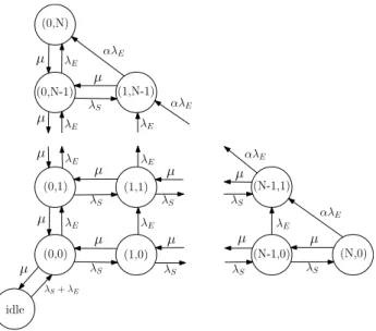
Fig. 1. State transition rate diagram for the STPQ.
3. Model description and preliminary results
We model the space–time priority queue as a non-preemptive priority queue with two classes of packets. Class-S (streaming) and class-E (elastic) packets arrive to the system according to a Poisson process of rate
λS
andλE
, respectively. We denote by fX the density function of a continuous random variable X . We assume that the service time distribution of both type of packets, denoted by the random variable B, is exponentially distributed with parameterµ
, i.e., fB(x)=
µ
e−µx. In particular, we have E(B)=
1/µ
. The buffer has finite size N and it is shared by both classes of packets. Thus, the total number of packets that can simultaneously be in the system is N+
1, that is, N in the buffer and one in service. We letLE(t) and LS(t) denote the number of class-E and class-S packets in the buffer at time t, respectively.
Class-S (streaming) packets have time priority over class E (elastic) packets. This implies that a class-E packet gets served only if LS(t)
=
0. If the buffer is not full, that is LS(t)+
LE(t)<
N, an incoming packet from either class is accepted into the buffer. Class-E packets have space priority over class-S packets. Thus, if the buffer is full, an incoming class-S packet will not be accepted into the buffer, and an incoming class-E packet will push-out from the queue the last class-S packet with probability 0≤
α ≤
1. The caseα =
1 is denoted as ‘‘non-randomized push-out’’, and it will be particularly present in our analysis. As we will see in the ensuing, the caseα <
1 is less amenable to analysis.Let pi,j
=
limt→∞P(LS(t)=
i,
LE(t)=
j) denote the steady-state probability that there are i+
j packets in the queue, out of which i are of type class-S and j are of type class-E. We also denote by pidle=
P(idle) the stationary probability that the server is idle. Under the just described modeling assumptions, (LS(t),
LE(t))t≥0is a Markov Chain, and the transition diagram characterizing the steady-state is depicted inFig. 1, which expands vertically with class-E packets and horizontally with class-S ones for at most N total packets. Note that downward transitions only happen in the first column, when no class-S packets are waiting and push-out transitions can only happen in the boundary LS(t)+
LE(t)=
N.Then, the steady-state probabilities are the unique solution of the following system of equations: (
λS
+
λE
)pidle=
µ
p0,0,
(
λS
+
λE
+
µ
)p0,0=
µ
p1,0+
µ
p0,1+
(λS
+
λE
)pidle,
µ
p0,N=
λE
p0,N−1+
αλE
p1,N−1,
(αλE
+
µ
)pN,0=
λS
pN−1,0,
(
λS
+
λE
+
µ
)p0,j=
µ
p1,j+
µ
p0,j+1+
λE
p0,j−1,
for 0<
j<
N,
(λS
+
λE
+
µ
)pi,0=
µ
pi+1,0+
λS
pi−1,0,
for 0<
i<
N,
(
λS
+
λE
+
µ
)pi,j=
µ
pi+1,j+
λS
pi−1,j+
λE
pi,j−1,
for 0<
i+
j<
N,
(αλE
+
µ
)pi,j=
λS
pi−1,j+
λE
pi,j−1+
αλE
pi+1,j−1,
for i+
j=
N.
We let pN
=
∑N
i=0pi,N−i denote the probability that there are N packets in total in the queue. The traffic intensities for each class are denoted byρS
=
λS/µ
andρE
=
λE/µ
, and thusρ = ρS
+
ρE
is the total intensity. It is easy to see thatpN
=
1
−
ρ
1−
ρ
N+2ρ
as the total number of packets in the buffer evolves as the buffer content of an M
/
M/
1/
N+
1 queue with arrival rateλS
+
λE
and service rateµ
. Similarly, we note that the total probability along diagonals can be directly retrieved from known formulas of the M/
M/
1/
N+
1 queue. Thus, the probability of having k packets is thenk
∑
i=0 pi,k−i=
(1−
ρ
)ρ
k+1 1−
ρ
N+2,
(1)while the idle and empty buffer probabilities equals,
pidle
=
(1
−
ρ
)1
−
ρ
N+2,
p0,0=
(1
−
ρ
)ρ
1−
ρ
N+2.
The main performance criteria we are interested in are the loss probabilities for both class-S, denoted by p(S)loss, and
class-E, p(E)loss, as well as the mean waiting times for both classes, denoted by, E
[
WS]
and E[
WE]
. These performance measures are determined in the following sections.4. Main results
In this section we state our main results regarding the performance criteria steady state probabilities, packet loss probabilities and mean waiting times for class-S and class-E packets.
4.1. Steady-state probabilities
The steady-state probabilities can be found by solving the system of balance equations. Since the Markov chain is finite and irreducible, the balance equations have a unique normalized solution. Computing the steady-state probabilities using matrix inversion can be computationally heavy when N grows. Exploiting the structure of the Markov chain, seeFig. 1, we however can calculate these probabilities more efficiently. The key for our approach is the observation that we can solve the steady state probabilities per row because: (i) downward transitions are only possible in the first column, i.e., in states with no class-S packets and (ii) we know the probability mass on the diagonals. The next proposition describes the algorithm to calculate the probabilities.
Proposition 1. The following algorithm finds the unique solution of the system of steady state equations in O(N2) steps:
1. Probabilities pi,0:
(a) Set bN
=
1 and bN−1=
αλE+µ
λS and recursively calculate
bi
=
bi+1λE
+
λS
+
µ
λS
−
bi+2µ
λS
for i=
N−
2, . . . ,
0.(b) Given the values bi, calculate
pi,0
=
bi b0 (1−
ρ
)ρ
1−
ρ
N+2,
for i=
0, . . . ,
N. 2. Probabilities pi,j, for j=
1, . . . ,
N:(a) Set a(j)N−j
=
0 and a(j)N−j−1= −
(pN−j,j−1+
α
pN−j+1,j−1)λλES, and recursively calculate for i=
N−
j−
2, . . . ,
0,a(j)i
=
a(j)i+1λE
+
λS
+
µ
λS
−
a (j) i+2µ
λS
−
pi+1,j−1λE
λS
,
(b) Calculate p0,j, p0,j=
(1−
ρ
)ρ
j+1 1−
ρ
N+2−
j∑
i=1 pi,j−i,
and for i
=
1, . . . ,
N−
j, calculate,pi,j
=
a(j)i+
bi+jp0,j
−
a(j)0bj
.
Remark 1. Proposition 1 can be easily extended to the case of state-dependent push-out probabilities, that is, when
αi
,
i=
1, . . . ,
N, depends on i, the number of class-S packets waiting. The latter can be of interest to reduce the push-outprobability when the number of class-S packets is small.
Carefully counting the number of operations, we find that the computational complexity of Algorithm1is O(N2). As the number of states is O(N2) one cannot do better if one wants to calculate all probabilities. We note however that it may be possible to find faster algorithms which are O(N2) as well.
Algorithm 1 Efficient algorithm for steady-state probabilities.
1: procedure Steadystate(N
, α, λS
, λE, µ
)2: b(N)
←
1 3: b(N−
1)←
(αλE+µ) λS 4: for i=
N−
2, . . . ,
0 do 5: b(i)←
b(i+
1)λE+λS+µ λS−
b(i+
2) µ λS 6: end for 7: for i=
0, . . . ,
N do 8: p(i,
0)←
b(i) b(0) (1−ρ)ρ 1−ρN+2 9: end for 10: for j=
1, . . . ,
N do 11: a(N−
j)←
0 12: a(N−
j−
1)← −
(p(N−
j,
j−
1)+
α
p(N−
j+
1,
j−
1))λE λS 13: for i=
N−
j−
2, . . . ,
0 do 14: a(i)←
a(i+
1)λE+λS+µ λS−
a(i+
2) µ λS−
p(i+
1,
j−
1) λE λS 15: end for 16: p(0,
j)←
(1−ρ)ρj+1 1−ρN+2−
∑j
i=1p(i,
j−
i) 17: for i=
1, . . . ,
N−
j do18: p(i
,
j)=
a(i)+
b(i+
j)p(0,j)b(j)−a(0)19: end for
20: end for
21: return p
22: end procedure
4.2. Loss probabilities
The expression for the loss probabilities is given in the following proposition.
Proposition 2. The loss probabilities of streaming and elastic packets are given by the following formulae
p(E)loss
=
p0,N+
(1−
α
)(pN−
p0,N),
(2) p(S)loss=
pN+
α
ρE
ρS
(pN−
p0,N),
(3) where pN=
1−
ρ
1−
ρ
N+2ρ
N+1.
Proof. An arriving elastic packet at time t will be lost either (i) when the buffer is full of elastic packets, LE(t)
=
N, or(ii) with probability 1
−
α
in case the buffer is full (LS(t)+
LE(t)=
N) and the number of streaming packets satisfies0
<
LS(t)≤
N. The probabilities of those events are p0,N and∑N
i=1pi,N−i, respectively. Thus, by the PASTA property(Poisson Arrivals See Time Averages) we obtain(2).
The stream of class-S packets lost is formed by two streams: those lost when the buffer is full, which happens at rate
λS
pN, and those lost by being pushed-out by class-E packets, which happens at rateαλE
(pN−
p0,N). Summing these two rates and equating withλS
p(S)loss, yields(3). □4.3. Waiting time
In this section we assume that the steady-state probabilities pm,nare known (seeProposition 1) and we show how to calculate the mean waiting time of both classes. The waiting time of interest is the one which takes into account only the packets that are actually served.
For the elastic traffic, since a job that enters the queue is never pushed out, we can apply Little’s Law to the number of elastic customers in the system. We note that in this case the effective arrival rate is
λE
(1−
p(E)loss). Thus, we concludethat
E [WE
|
served]=
E[
LE]
λE
(
1−
p(E)loss) .
(4)The waiting time for the class-S packets is considerably more complicated since a packet that enters the queue can be lost later on. We now consider a tagged class-S packet waiting in the queue and define the following mean waiting time, conditioned on the number of class-E packets and the number of class-S packets before and after the tagged packet in the queue,
w
(m,
m′,
n)=
E[
WS1{served}|
m class-S before, m ′class-S after, n class-E
]
.
By the PASTA property, the probability that an arriving packet finds LS(t)
=
m class-S and LE(t)=
n class-E packets on arrival is pm,n. ThusE
[
WS1{served}] =
∑
m,n
w
(m,
0,
n)pm,nand by the conditional probability formula it holds E [WS
|
served]=
∑
m,n
w
(m,
0,
n)pm,n 1−
p(S)loss.
(5) The following proposition shows how to calculate the values
w
(m,
m′,
n). The proof is inAppendix B.
Proposition 3. The conditional mean waiting times
w
(m,
m′,
n),
m+
m′+
n≤
N−
1 satisfy the recursive formulasw
(m,
m′,
n)=
∑
i+j≤N−m−m′−n−2 gij(
cij+
w
(m−
1,
m ′+
i,
n+
j))
+
∑
i+j=N−m−m′ −n−1 k≤i+m′vijk
(
dijk+
w
(m−
1,
m ′+
i−
k,
n+
j+
k))
w
(0,
m′,
n)=
∑
i+j≤N−m−m′−n−2 gijcij+
∑
i+j=N−m−m′ −n−1 k≤i+m′vijk
dijk where gij=
(
i+j i)
λiSλjEµ (λS+λE+µ)i+j+1, cij=
λi+j+1 S+λE+µ,vijk
=
(
i+j i)
λiSλjE (λS+λE+µ)i+j (αλE)kµ (αλE+µ)k+1 and dijk=
λ i+j S+λE+µ+
k+1 αλE+µ. The aboverecursion finds the conditional mean waiting times
w
(m,
m′,
n) in O(N4) steps.
In the special case when
α =
1,w
(m,
m′,
n) does not depend on m′
, that is, the number of class-S packets that are in the queue after the tagged job do not affect the probability that the tagged job is served. Bear in mind that new class-E packets are not affected by them. In this case, the waiting time will only depend on the number of class-S jobs ahead of the tagged job, and the number of class-E jobs in the system. The waiting time could be calculated using Eq.(5)and Proposition 3. However, we can develop a more efficient algorithm by taking advantage of
w
(m,
n)=
w
(m, ·,
n). Proposition 4.w
(m,
n) satisfies:w
(m,
n)=
N−n−m−1∑
k=0 (fk+
w
(m−
1,
n+
k)gk),
w
(0,
n)=
N−n−1∑
k=0 fk, w(idle)=
0 where fk=
λ k Eµ (λE+µ)k+2(k+
1) and gk=
λ k Eµ(λE+µ)k+1. The recursive formulas are solved by index m (from 0 to N).
Proof. We assume that the streaming packet that entered last will be pushed out first. First of all, letP be a Poison process with unitary rate and consider the formula
gk
=
E[
1{P(λEB)=k}] =
∫
∞ 0 (λE
t)k k!
e −λEtf B(t)dt=
∫
∞ 0 (λE
t)k k!
e −λEtµ
e−µtdt=
∫
∞ 0µ
e−z (λE
λ z E+µ) k k!
dzλE
+
µ
=
λ
k Eµ
(λE
+
µ
)k+1k!
Γ(k+
1)=
λ
k Eµ
(λE
+
µ
)k+1,
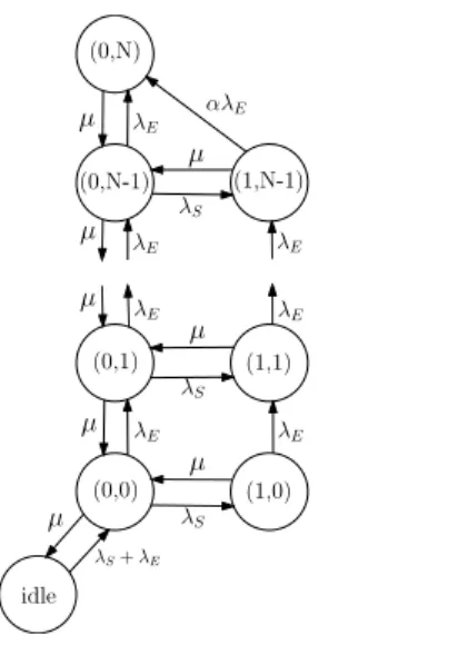
Fig. 2. State transition rate diagram for the light-traffic model. The diagram is a cut from the original STPQ where there will be at most two S
packets in the system.
whereΓ(
·
) is the Gamma function. The formula gkexpresses the probability that exactly k class-E packets arrive during a service time. Similarly, we obtainfk
=
E[
B1{P(λEB)=k}]
=
λ
k Eµ (λE
+
µ
)k+2(k+
1).
that gives the mean waiting time of the event defined by gk, which takes k
+
1 steps with mean length (λE
+
µ
)−1. It is clear thatw
(idle)=
0, since a packet that arrives when the server is idle enters the service. Now, consider m=
0, when no streaming packet is waiting in the queue. In this case, the arriving class-S packets will receive service if at mostN
−
n−
1 elastic packets arrive before the one in service leaves. Thus, we can consider every described possibility and sum over them:w
(0,
n)=
N−n−1∑
k=0 fk. For m≥
1, consideringw
(m′,
n) are known for every m′
<
m, note that being at state (m
,
n) and k elastic arrivals happenin a service time moves the system to the state (m
−
1,
n+
k). With this, considering a streaming arrives at state (m,
n)and knowing the probabilities that k elastic packets arrive (gk), and the length of the service (fk), we can derive
w
(m,
n)=
N−n−m−1
∑
k=0
(fk
+
w
(m−
1,
n+
k)gk),
which can be computed since
w
(m−
1,
n+
k) are known from the previous steps. Solving for each m all thew
(m,
n), wecan do it again for m
+
1, until the system is completely solved. □5. Light-traffic approximation
The light-traffic regime aims at approximating the steady-state performance when the traffic load is extremely low. More precisely, we will consider the regime in which
λS
→
0, without making any assumption on the value ofλE
. As explained in the introduction, recent empirical measurements indicate that the arrival rate of streaming packets is much lower than that of elastic, and we can thus expect the light-traffic regime to be a good approximation in case the load due to streaming traffic is low. This approximation was pioneered in [23], see also [24]. In this regime, the number of jobs in the system will be very small. In particular, as shown in [24], the first-order light-traffic approximation is obtained by analyzing the original system in which at most one job may arrive. To explain this intuitively, note that ifλS
is very small, the probability of having two class-S arrivals is of order o(λ
2S), and thus negligible.
The goal of this section is to approximate the loss probabilities for both classes of packets, which from(2),(3), required finding p0,N. The state transition rate diagram under the light traffic assumption is depicted inFig. 2.
To solve the steady-state in the light-traffic regime, we will use known results from analytic perturbation theory applied to Markov Chains, see [25]. It is known that if the transition rate matrix and the equilibrium probabilities are
of the form Q (
ϵ
)=
Q0+
ϵ
Q1+
ϵ
2Q2+ · · ·
andπ
(ϵ
)=
π
0+
ϵπ
1+
ϵ
2π
2+ · · ·
, then the steady-state probabilities can be obtained by solving the system of fundamental equationsπ
0Q0=
0π
1Q0+
π
0Q1=
0...
πk
Q0+
πk
−1Q1+ · · · +
π
1Qk−1+
π
0Qk=
0...
together with the system normalization conditionsπ
01=
1πk
1=
0,
k≥
1We will apply this characterization to our queueing model. For our situation, with the state space ordered
{
idle,
(0,
0),
(0,
1), . . . ,
(0,
N−
1),
(0,
N),
(1,
0),
(1,
1), . . . ,
(1,
N−
2),
(1,
N−
1)}
the transition rate matrix QLT can be written asQLT(
λS
)=
Q0+
λS
Q1,
where Q0=
⎛
⎜
⎜
⎜
⎜
⎜
⎜
⎝
QEM/M/1/N+1 0 0µ
... ...
0µ αλE
−
(λE
+
µ
)λE
...
...
−
(αλE
+
µ
)⎞
⎟
⎟
⎟
⎟
⎟
⎟
⎠
and Q1=
⎛
⎜
⎜
⎜
⎜
⎜
⎜
⎜
⎜
⎜
⎜
⎝
−
1 1−
1...
−
1 0 0. . .
0 1...
1 0 0 0⎞
⎟
⎟
⎟
⎟
⎟
⎟
⎟
⎟
⎟
⎟
⎠
,
where QEM/M/1/N+1denotes the transition rates of an M
/
M/
1/
N+
1 queue with only class-E packets.We are interested in approximating the only unknown term in the loss probability equations(2),(3), which is p0,N. In the light-traffic regime, pN will be composed by p0,N
+
p1,N−1. From our knowledge of pN from the M/
M/
1/
N+
1 system and the light-traffic approximation for p1,N−1developed in the followingLemma 1, we can obtain an approximation for p0,N. The proof is deferred toAppendix C.Lemma 1. The light-traffic approximation of the STPQ queue for p0,N is
pLT0,N
=
pN−
pLT1,N−1 (6) where pLT1,N−1=
λS
αλE
+
µ
1−
ρE
1−
ρ
NE+2(
ρ
N−1 E−
(
λE
λE
+
µ
)N
−1+
ρ
NE)
The accuracy of the light-traffic approximation for different system configurations is analyzed in Section6.3.
6. Numerical results
6 0.4
'g
è:. 4 0.3!ilJ
0,2 C.�
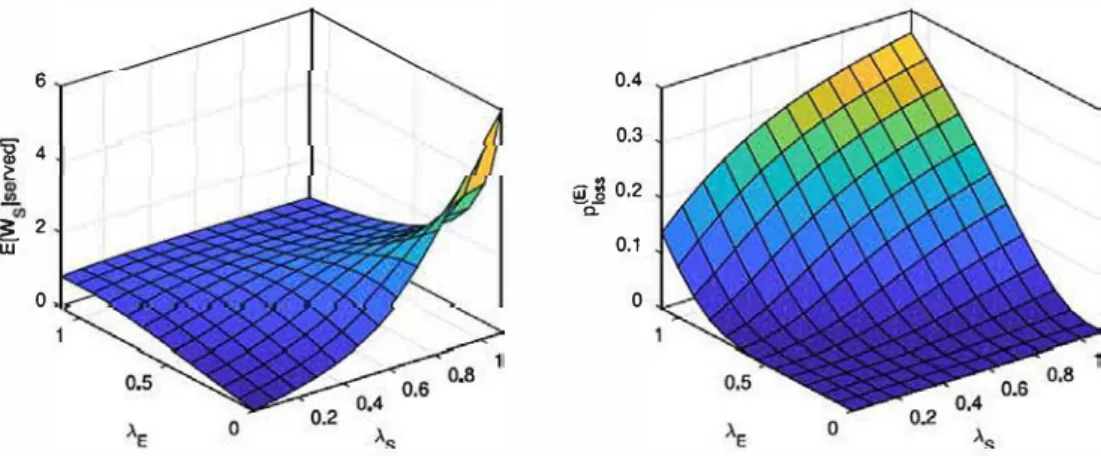
2 w 0.1 0 0Fig. 3. Mean waiting lime (left) and loss probability (right) in the non-randomized push-out STPQ (a
=
1) with N=
10, µ,=
1 and dilferent traffic configurations. 3.5---�---3i
2.5""
0, .!:; 2 ·� � 1.5 � 1 --E[W 51served] -·---E[WElserved] ... E[WM/M/1/N•I] 0 .._ __ .._ __ ..._ __ ...._ __ ...._ __ _, 0.3 0.4 0.5 0.6 0.7 0.8 ). 0.04 ---�---0.035 � 0.03 :02
0.025 ::! 0.02 .!2j
0,015a
0.01 0.005--
pt!.
-·---p�
.....!
.
... P;:111/N•I 0 L---...---
=
==:.:.;_
__ ...._ __
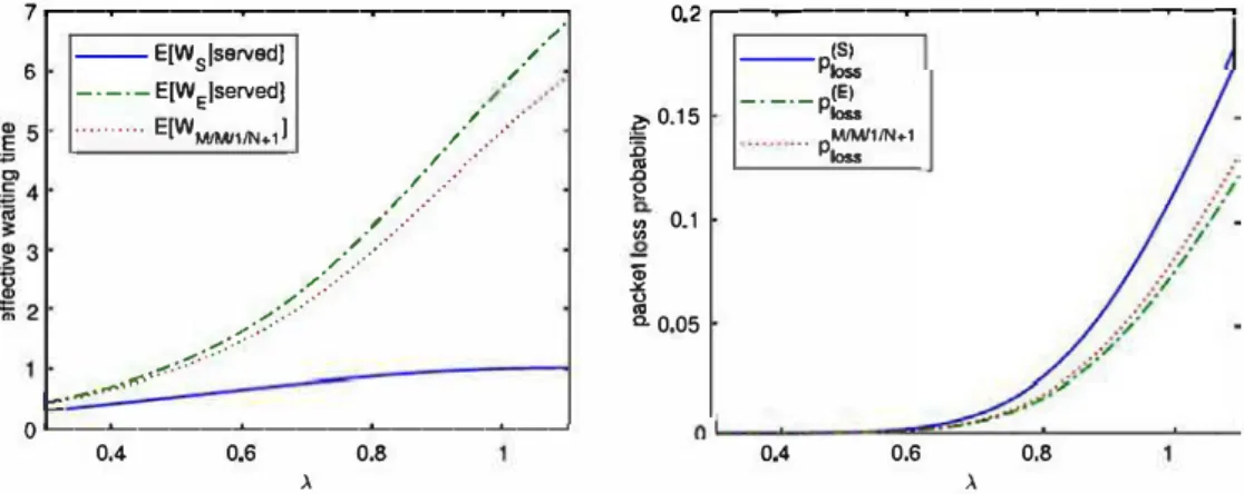
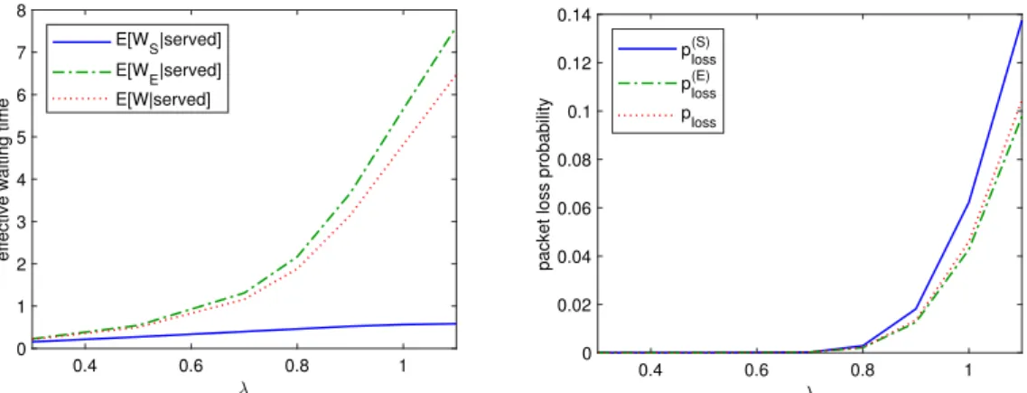
....J 0.3 0.4 0.5 0.6 0.7 0.8Fig. 4. Mean waiting cime (left) and loss probabilicy (right) with N
=
10 and a= 1. Proportion or traffic satisfies J..5/J..E=
0.2 and total arrivai rate is }, = Às + ÀE.6.1. Case a= 1
ln this subsection we study the loss probability and the waiting time in the case
a
=
1.As we can see in Fig. 3 (left), the mean waiting time for streaming packets remains low over almost every configuration
of the system. When elastic traffic is close to 0, the waiting time is increasing on À.s, since we would be just dealing with
an M /M /1/N + 1 queue for class-S. We also see that when the arrivai rate of both classes is high, the waiting time for the streaming packets that are not pushed-out does not increase. Even if class-E traffic is high, we observe that the waiting time of class-S does not increase significantly. This is due to the fact that we measure the waiting time conditioned on the packet being served. Thus, we observe that the only scenario in which class-S packets have a large waiting time is
when À.s is large.
ln Fig. 3 (right) we plot the loss probabilities for different configurations. We observe that for small to moderate values of À.f, the loss probability of class-E packets is fairly insensitive to the value of À.s.
As in (3), we now assume that the ratio of streaming traffic over elastic traffic is fJXed with value À.s/ÀE
=
0.2. Numerical results of this scenario for different traffic intensities can be observed in Fig. 4. ln Fig. 4 (left), it can be seen that, while traffic becomes high, waiting time for streaming class is much lower than the one in the system without priorities, that is, the M /M /1/N
+ 1 system. Moreover, the waiting time for elastic packets is not much bigger than in the non priority queue. Then, in Fig. 4 (right), the loss probabilities are represented for the same parameter settings. There, it is seen that for high arrivai rates, the performance of elastic traffic regarding the Joss probability improves with respect to non priority system, and that the contrary holds for the streaming packets.6.2.
The
case
O :'.::
a
:'.::
1
By varying the traffic rates of streaming and elastic class packets, À.s and À.f, we consider different scenarios to analyze
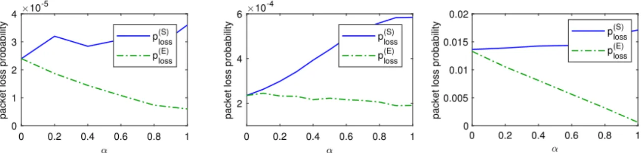
Fig. 5. Loss probabilities for the STPQ with parameters N=10 andµ =1 with respect to the push-out probabilityαfor different traffic configurations.
λS=λE=0.3 (left),λS=0.2, λE=0.5 (center) andλS=0.7, λE=0.2 (right).
Scenario 1: similar traffic intensities
We suppose in this first scenario that we are dealing with similar traffic intensities for both streaming and elastic packets. We let the parameters be N
=
10, λS
=
0.
3, λE
=
0.
3, µ =
1.For a situation in which the total amount of traffic intensity is low, seeFig. 5(left), loss probabilities are of order 10−3 for both classes. As we can see, while
α
grows from zero to one the increase of class-S loss probabilities and the decrease of class-E loss probabilities are roughly of the same order.We should note that the loss probabilities are the same for both types of traffic when
α =
0. In that situation there is no push-out, so every packet that arrives when the buffer is full will be refused. Thus, the loss probability does not depend on the incoming packet class, only on the resulting traffic rate (and the size of the buffer). Moreover, this loss probability is the probability that M/
M/
1/
N+
1 is full, given by pN.We conclude that in this scenario where streaming and elastic traffic is similar, the parameter
α
can be adapted in order to reduce the probability for one class whereas for the other class is increased. This allows the controller to reduce the loss probability for one class without sacrificing the other class traffic.Scenario 2: higher traffic intensity of streaming packets
In this scenario we analyze the situation in which
λS
> λE
. We consider for this scenario N=
10, λS
=
0.
7, λE
=
0.
2, µ =
1. InFig. 5(right) we can see that the behavior in not the same as in Scenario 1. The relevant property of thisscenario is that increasing the push-out probability improves a lot the loss probability of class-E packets without having a great impact into the class-S packets.
Scenario 3: higher traffic intensity of elastic packets
In this scenario we take the parameters N
=
10,λS
=
0.
2,λE
=
0.
5,µ =
1. In this case, enabling the push-out mechanism with a high probabilityα
reduces the probability of losing class-E packets but the price is high for class-S packets. We can see again inFig. 5(center) how, with the growth ofα
, the loss probability for streaming packets increases very fast in comparison to the loss probability reduction for elastic packets.In addition to the loss probabilities, we also consider the waiting times of class-S and class-E packets in the case of 0
≤
α ≤
1. In Fig. 6we consider the same traffic configuration as inFig. 4, but withα =
0.
3. Comparing the results with respect to the non-priority case, that is, the M/
M/
1/
N+
1 case, we see that (left) the mean waiting time of class-S packets improves considerably whereas (right) the degradation of the loss probability of class-S packets is less significant than in the caseα =
1. InFig. 7we plot the waiting time of class E and S packets. We observe that the waiting time is largely insensitive to the value ofα
. Thus, it can be concluded that the push-out probability parameterα
gives flexibility to optimize the waiting time of streaming packets, while keeping control of the blocking probability of class-E packets.The results ofFig. 7also suggest that instead of making use of the algorithm proposed inProposition 3, the waiting time could be efficiently approximated by a linear interpolation between the values for
α =
0 andα =
1. The caseα =
0, that is, the finite queue with time-priority, can be computed using the Little’s law for class-S packets because in this particular case, any of those packets that enter the queue will receive service. Forα =
1, the algorithm proposed in Proposition 4may be used.6.3. Accuracy of light-traffic approximation
We analyze now the accuracy of our light-traffic approach. InFig. 8(left) we consider a scenario where the proportion
of class-S packets over class-E ones is 0.15. We observe that the error for class-S packets is higher than for class-E packets, but the approximation is considerably accurate in both cases. InFig. 8(right) we consider a scenario with the proportion
1---6 --E[W51served] -• -· -E[W elserved) .......... E[WMIW1/N+1] / / / /
..
· /.
.
.
··
/ _..
··
/ _.-' / .. ··,,.
<
:..-
·
·
·
/·..
··
, .... ,«:,-:-::.".'.:. -'.'-:-�:-··' �\f"'\.-
-
-�
o�-�---�---�---�-�
0.4 0.6 0,8 À 0.2 ---�0.15�
�
gi 0.1�
a. 0,05 --pi! -----p� ... p=I/N+I 0.4 0,6 0,8 ÀFig. 6. Mean waiting time (left) and toss probability (right) or t.he STPQ wit.h N = 10, µ = 1 and a = 0.3. Toe arrivai rare is À= Às + Àf with
Às/Àe = 0.2. 1.5 10 8
î
I
65:
w
�
0.5�
w 2 0 0 1 1 1.5 1.5 a 0 0 Q 0 0 ).Fig. 7. Mean waiting time for class-S (left) and class-E (right) packers wirh N = 10, µ = 1 and a proportion or traffic Às/ÀE = 0.25, with rotai
arrivai rate À = Às +
Àe-0.3
f
0.25�
lS. 0,2=
.!i! 0.151
'" 0.1 Q. 0.05 -e-p:s (LT) -e, -pf! -p�8(LT) -e--p�O�-ê'--E,...D,!!oéli!::
:::::::'.'.._��-�-0.4 0.5 0.6 0.7 0.8 0.9 À 1.1 1.2 0,35 0.3 ,§0.25
..
�
Q.=
0.2 SI 0.15I
0.1 0.05 0.4 -e-p�� (LT) -e, -p�� -p:�(LT) -e--p:� 0.5 0.6 0.7 0.8 À 0.9 1.1 1.2Fig. 8. Light-traffic approximation performance 011er loss probabilities for both class-S and class-E packets on a system wit.h parameters N = 10, µ = 1 and a= 0.8. The arrivai rate is À= Às + Àe with proportions sarisfying (left) Às/Àe = 0.15 and (right) Às/ÀE = 0.3.
to a configuration in which class-S traffic is not as light as it was in the previous configuration. We note that this traffic
ratio is considerably more balanced than the one observed in real traces.
7. Simulation results
ln this section, results of simulations are presented to evaluate scenarios where previously stated assumptions do
not hold. We program a simulator in order to assess the performance of STPQ with non-Markovian assumptions for two
different scenarios, one considering deterministic packet sizes and the other from a real trace.
Fig. 9. Loss probabilities for the STPQ with parameters N=10 and deterministic service times (size 1) with respect to the push-out probabilityα for different traffic configurations.λS=λE=0.3 (left),λS=0.2, λE=0.5 (center) andλS=0.7, λE=0.2 (right).
Fig. 10. Mean waiting time (left) and loss probability (right) with N =10,α =1 and deterministic service times (size 1). Proportion of traffic satisfiesλS/λE=0.2 and total arrival rate isλ = λS+λE.
7.1. Deterministic packet sizes
Throughout this subsection, it is considered that packets arrive under the Markovian assumption and that packet sizes are deterministic of size 1.
Fig. 9shows the loss probability for the same parameters as the ones considered inFig. 5. Comparing the two sets of figures, it can be seen that the curves show qualitatively a similar shape, with loss probabilities increasing and decreasing in similar proportions for the Markovian and non-Markovian settings, and that in the deterministic case it is less likely to loss packets, which is expectable due to the lower variability of the deterministic service time distribution.
Similar conclusion can be drawn when comparing the performance as a function of the arrival rate, seeFigs. 10and11 for deterministic packet sizes andFigs. 4and6for exponentially distributed packets. While loss probabilities are lower as a function of the arrival rate, the effective waiting time does not show the same pattern. For low arrival rates, the waiting time is smaller with deterministic packets sizes, but as the arrival rate increases, for example greater than 1 inFig. 11, class-E packets have to wait more in the case packets are deterministic.
Having analyzed the different scenarios for the STPQ with deterministic service times, we conclude that the formulas derived for the Markovian setting provide a good baseline to estimate the qualitative behavior of the STPQ.
7.2. Real trace from WIDE
In this subsection we consider a trace from WIDE with measurements from 2019/01/02, see [4]. The data set we consider is formed by 5 million packets, from which 95% are TCP (type E) and the remaining 5% UDP (type S). InFig. 12 we visualize the distribution of the (left) packet inter-arrival time and the (right) packet size. We observe that the inter arrival time for TCP packets is much smaller, which is expected given that 95% of the packets TCP. Another interesting observation is that TCP packets are significantly larger than UDP ones. For the simulation, we consider a server with speed 1 Gigabyte per second as specified in the source of the trace, and the buffer size was chosen to be N
=
4 so that the impact of the push-out probability parameterα
can be observed.Fig. 13shows the performance of the STPQ for the defined trace. In (left) we see that the waiting time of class-S or UDP packets is considerably smaller than that of class-E or TCP packets. We also note that the choice of
α
does not haveFig. 11. Mean waiting time (left) and loss probability (right) of the STPQ with N=10, deterministic service times (size 1) andα =0.3. The arrival rate isλ = λS+λEwithλS/λE=0.2.
Fig. 12. Complementaries of the cumulative distribution functions of seconds between packet arrivals (left) and size of packets in seconds (right) of
the real trace of 5 million packets considered to simulate the STPQ.
Fig. 13. Mean waiting time (left) and loss probability (right) of the STPQ with N=4 for a real trace of 5 million packets processed at a rate of 1 Gigabyte per second.
much of an impact. On the (right) we see that the packet loss probability clearly increases on
α
for UDP traffic, whereas it decreases at a lower rate for TCP packets.These observations regarding the impact of
α
coincide qualitatively, under similar choice of other parameters, with the predictions of our mathematical model for the Markovian setting.8. Conclusions
In this paper we have introduced and studied the space–time priority queue (STPQ), where one class has time priority, whereas the other one has space priority. The main motivation of STPQ is to model the performance of scheduling algorithms that can provide service priority to streaming type of packets (say UDP traffic in the Internet) and space priority to elastic type of packets (say TCP). In the literature such scheduling algorithms have been previously proposed, see [5,6], but to the best of our knowledge, our work is the first attempt to propose a queueing model to analyze it. In our main contribution we have derived algorithms to calculate efficiently the loss probabilities and the mean waiting time. The
numerical examples show that STPQ permits, comparing to a queue without priorities, to provide a lower delay to class-S packets without a significant degradation of the performance of class-E packets.
Declaration of competing interest
No author associated with this paper has disclosed any potential or pertinent conflicts which may be perceived to have impending conflict with this work. For full disclosure statements refer tohttps://doi.org/10.1016/j.peva.2019.04.003.
Appendix A. Proof ofProposition 1
We recall from Section3that the total probability along diagonals are known, as well as pidleand p0,0. We first focus on the balance equations for states (1
,
0) to (N,
0). We have,pi,0(
λE
+
λS
+
µ
)=
pi+1,0µ +
pi−1,0λS
,
i=
1, . . . ,
N−
1,
pN,0(
αλE
+
µ
)=
p0,N−1λS
.
As p0,0 is already known, we have N equations and N unknowns. We will solve the system in O(N) (i.e. linear order complexity). We put p0,N in the following form
p0,N
=
β
p0,0Then, from the balance equations it follows that
pN−1,0
=
pN,0αλE
+
µ
λS
=
αλE
+
µ
λS
β
p0,0,
pN−2,0=
pN−1,0λE
+
λS
+
µ
λS
−
pN,0µ
λS
=
(
αλE
+
µ
λS
λE
+
λS
+
µ
λS
−
µ
λS
)
β
p0,0,
...
In other words, if we define bi for i
=
N to i=
0 with the following recursion,bN
=
1,
bN−1=
αλE
+
µ
λS
bi=
bi+1λE
+
λS
+
µ
λS
−
bi+2µ
λS
.
then pi,0=
biβp0,0.
From the equation for the case of p0,0we can derive the value of
β
.β =
1 b0.
So, if we letβ
0=
p0,0 b0=
(1−
ρ
)ρ
b0(1−
ρ
N+2)it is verified that the values pi,0
=
biβ0solve the system of equations.We can now follow a similar procedure for the following rows in the transition diagram. For the j-th row, we can assume that we know all probabilities pi,kfor k
<
j. Moreover, we can determine p0,jby summing the jth diagonal,p0,j
=
(1−
ρ
)ρ
j+1 1−
ρ
N+2−
j∑
i=1 pi,j−i.
The N−
j equations we consider are,pi,j(
λE
+
λS
+
µ
)=
pi+1,jµ +pi−1,jλS+
pi,j−1λE
pN−j,j(
αλE
+
µ
)=
pN−j−1,jλS+
pN−j,j−1λE
+
pN−j+1,j−1αλE
For these equations, we conclude that it will not be a proportional rule for the states of the row since there is a dependency over the probabilities solved in other rows. Thus, we will have now
To solve these equations in O(N
−
j) we go downwards as we did for the first row. We have to calculate the values a(j)iand b(j)i by the recursion,
a(j)i
=
a(j)i+1λE
+
λS
+
µ
λS
−
a (j) i+2µ
λS
−
pi+1,j−1λE
λS
,
b(j)i=
b(j)i+1λE
+
λS
+
µ
λS
−
b (j) i+2µ
λS
,
with initial values,a(j)N−j
=
0,
a(j)N−j−1= −
(pN−j,j−1+
α
pN−j+1,j−1)λE
λS
,
b(j)N−j=
1,
b (j) N−j−1=
αλE
+
µ
λS
.
Noting that the solution to the recursion b(j)i is b(j)i
=
bi+jand then introducing the factorβj
,βj
=
p0,j−
a(j) 0 bj
,
one verifies that the set of equations is solved by the probabilities pi,j
=
a(j)i+
bi+jβj .Appendix B. Proof ofProposition 3
Let us consider the situation where the tagged packet is at state (m
,
m′,
n), for m+
m′+
n≤
N−
1. The value of interest isw
(m,
m′,
n)=
E[
WS1{served}
|
m class-S before, m ′class-S after, n class-E
]
.
We will write a recursive equationw
(m,
m′,
n) by keeping track of the arrivals during the service time.
We first consider the case when the queue is not full when the service time finishes, that is, m
+
1+
m′+
n
+
i+
j≤
N−
1,where i is number of arrivals of class-S, and j arrivals of class-E. Let us denote by gijthe probability that during the service time there are i arrivals of class-S and j arrivals of class-E, i.e.,
gij
=
E[
1{P(λSB)=i,P(λEB)=j}]
,
wherePdenotes a Poisson process with unitary rate. Similarly we also define
fij
=
E[
B1{P(λSB)=i,P(λEB)=j}]
.
Consider now that at the time of the next service, the queue is full, that is, there has arrived i type S and j type E arrivals with m
+
1+
m′+
n
+
i+
j=
N. Let Si+jbe the random variable denoting the time of the i+
j-th arrival of a Poissonprocess with rate
λS
+
λE
, and letvijk
the probability that during a service time i class-S and j class-E packets arrive, and that additional k class-E packets push-out a class-S packet, i.e.,vijk
=
E[
1{P(λSSi+j)=i,P(λESi+j)=j,Si+j<B,P(αλE(B−Si+j))=k}]
.
Similarly, we define:uijk
=
E[
B1{P(λSSi+j)=i,P(λESi+j)=j,Si+j<B,P(αλE(B−Si+j))=k}]
.
We can now write the recursion:w
(m,
m′,
n)=
∑
i+j≤N−m−m′−n−2(
fij+
gijw(m−
1,
m′+
i,
n+
j))
+
∑
i+j=N−m−m′ −n−1 k≤i+m′(
uijk+
vijkw
(m−
1,
m ′+
i−
k,
n+
j+
k))
(B.1) together withw
(m,
m′,
n)
=
0 for m<
0. This provides a set of recursive formulas over m, from zero to N−
1, to compute the values ofw
(m,
m′,
n).We now calculate the expressions for fij, gij,
vijk
and uijk.fij
=
E[
B1{P(λSB)=i,P(λEB)=j}] =
∫
∞ 0 tfB(t)P(P(λS
t)=
i,
P(λE
t)=
j)dt=
∫
∞ 0 tµ
e−µtP(P(λS
t)=
i)P(P(λE
t)=
j)dt=
∫
∞ 0λ
i Sλ
j Eµ
i!
j!
t i+j+1e−(λS+λE+µ)tdt=
λ
i Sλ
j Eµ
i!
j!
(λS
+
λE
+
µ
)i+j+1∫
∞ 0 zi+j+1e−zdz=
λ
i Sλ
j Eµ
i!
j!
(λS
+
λE
+
µ
)i+j+1Γ(i+
j+
2)=
(
i+
j i)
λ
i Sλ
j Eµ(i+
j+
1) (λS
+
λE
+
µ
)i+j+2,
i≥
0,
j≥
0,
whereΓ(·
) is the Gamma function. Similarly,gij
=
E[
1{P(λSB)=i,P(λEB)=j}] =
∫
∞ 0 fB(t)P(P(λS
t)=
i,
P(λE
t)=
j)dt=
λ
i Sλ
j Eµ
i!
j!
∫
∞ 0 ti+je−(λS+λE+µ)tdt=
(
i+
j i)
λ
i Sλ
j Eµ
(λS
+
λE
+
µ
)i+j+1,
i≥
0,
j≥
0.
We now proceed similarly to calculate uijkandvijk
. We haveuijk
=
E[
B1{P(λSSi+j)=i,P(λESi+j)=j,Si+j<B,P(αλE(B−Si+j))=k}]
=
∫
∞ 0 tfB(t)∫
t 0fSi+j|P((λS+λE)s)=i+j(s)P(P(
λS
s)=
i)P(P(λE
s)=
j)P(P(αλE
(t−
s))=
k)dsdt=
∫
∞ 0 tµ
e−µt∫
t 0 i+
j sλ
i Sλ
j Esi +je−(λS+λE)s i!
j!
(αλE
)k(t−
s)ke−αλE(t−s) k!
dsdt=
λ
i Sλ
j E(αλE
) kµ
(i+
j) i!
j!
k!
∫
∞ 0 si+j−1e−(λS+λE)s∫
∞ s te−µt(t−
s)ke−αλE(t−s)dtds=
λ
i Sλ
j E(αλE
)kµ
(i+
j) i!
j!
k!
∫
∞ 0 si+j−1e−(λS+λE+µ)s∫
∞ 0 (s+
z)zke−(αλE+µ)zdzds=
λ
i Sλ
j E(αλE
)kµ
(i+
j) i!
j!
k!
∫
∞ 0 si+j−1e−(λS+λE+µ)s(
sΓ(k+
1) (αλE
+
µ
)k+1+
Γ(k+
2) (αλE
+
µ
)k+2)
ds=
λ
i Sλ
j E(αλE
)kµ
(i+
j) i!
j!
(αλE
+
µ
)k+1∫
∞ 0 si+j−1e−(λS+λE+µ)s(
s+
k+
1αλE
+
µ
)
ds=
λ
i Sλ
j E(αλE
)kµ
(i+
j) i!
j!
(αλE
+
µ
)k+1(
Γ (i+
j+
1) (λS
+
λE
+
µ
)i+j+1+
k+
1αλE
+
µ
Γ(i+
j) (λS
+
λE
+
µ
)i+j)
=
(
i+
j i)
λ
i Sλ
j E (λS
+
λE
+
µ
)i+j (αλE
)kµ
(αλE
+
µ
)k+1(
i+
jλS
+
λE
+
µ
+
k+
1αλE
+
µ
)
,
i≥
0,
j≥
0,
k≥
0 andvijk
=
E[
1{P(λSSi+j)=i,P(λESi+j)=j,Si+j<B,P(αλE(B−Si+j))=k}]
=
∫
∞ 0 fB(t)∫
t 0fSi+j|P((λS+λE)s)=i+j(s)P(P(