AND
ASTROPHYSICS
Revised masses of
α Centauri
D. Pourbaix1, C. Neuforge-Verheecke2,?, and A. Noels2
1 Institut d’Astronomie et d’Astrophysique, Universit´e Libre de Bruxelles, C.P. 226, Boulevard du Triomphe, B-1050 Bruxelles, Belgium 2 Institut d’Astrophysique et de G´eophysique de l’Universit´e de Li`ege, Avenue de Cointe 5, B-4000 Li`ege, Belgium
Received 7 October 1998 / Accepted 7 January 1999
Abstract. With the precise radial velocities lately published
(Murdoch et al., 1993), a simultaneous least-squares adjust-ment of all visual and spectroscopic observations of theα Cen-tauri system is now possible and likely to yield some accurate information. Such an orbit determination leads to a mass ratio in agreement with the astrometric estimate of Kamper & Wes-selink (1978) but yields upward revisions of the distance and masses. We examine the effects these revisions on the evolu-tionary status of the system.
Key words: stars: binaries: spectroscopic – stars: binaries:
vi-sual – stars: fundamental parameters – stars: individual:α Cen
1. Introduction
α Cen is the binary system closest to the Earth and one could think it has been studied so intensively that there is nothing new to discover. It is true that it has been visually measured for almost 250 years but its long period coupled to the poor quality of the spectroscopic measurements leads to a surprisingly large remaining uncertainty on the individual masses. Precise radial velocities lately published (Murdoch et al., 1993) have radically changed the situation. Coupling them to visual observations, one derives significant upward revisions of the distance and masses.
2. Orbits, mass ratios and parallaxes
α Cen has been subject to many independent investigations about its mass ratio, parallax ($) and system’s radial velocity for almost 100 years. Most have lead to discrepant results (e.g., the astrometric and spectroscopic mass ratios do not agree).
One needs the mass sum and the mass ratio to derive the in-dividual masses. The former comes out of the visual orbit when the parallax is known whereas the latter can be derived from ei-ther astrometric or spectroscopic observations. The most recent mass determinations are based on astrometric investigations, the quality of the radial velocities ofα Cen being rather poor.
The visual orbit quoted as the reference par excellence is still the one by Heintz (1958) (and then lately published again
Send offprint requests to: D. Pourbaix ([email protected])
? Charg´e de Recherches of the Belgian Fund for Scientific Research
(Heintz, 1982)) even if neither takes the last 40 years of visual observations into account. For the mass ratio, the most trusted one is due to Kamper & Wesselink (1978). They derivedκ =
0.454 ± 0.002 (κ ≡ MB/(MA+ MB)) and $ = 750 ± 5
mas. These values coupled to Heintz’ yieldMA = 1.10M
andMB = 0.91M . A slightly different choice of the weights
lead Demarque et al. (1986) to$ = 750.6 ± 4.6 mas. From some theoretical considerations only, Neuforge-Verheecke & Noels (1998) have lately proposedMA= 1.12M andMB =
0.94M .
Though only three years are covered by the observations of Murdoch et al. (1993), they are precise enough to estimate a reliable spectroscopic mass ratio. Murdoch & Hearnshaw (1993) used these radial velocities to determine MB/MA =
0.75 ± 0.09, just at the limit of consistency with the solution by
Kamper & Wesselink (1978).
The wayα Cen has been considered in the observation re-duction process after Hipparcos (ESA, 1997) may be question-able. Owing to the slow apparent orbital motion of B between 1989.9 and 1993.2, both components have been reduced with the (default) single star model. The two stars were not considered as being the members of a binary system in most of the reduction. The only exception was the assumption of the uniqueness of the parallax. That yielded a solution for both components qualified as uncertain (sic). Multiple solutions are proposed. The adopted parallax,742 ± 1.42 mas, is lower than all previous estimates.
3. Simultaneous spectro-visual adjustment
Instead of disjoint determinations of the visual orbit, the mass ratio and the parallax, one can advantageously undertake a si-multaneous adjustment of all visual and spectroscopic observa-tions (Morbey, 1975; Pourbaix, 1998). We therefore include all visual observations from the Washington Double Star Catalog (US Naval Observatory), photographic as well as micrometric, and the radial velocities from the end of last century up to those of Murdoch et al. (1993).
In order to combine radial velocity sets, we put them in the same reference frame (by adding the same correction (cf. Table 1) to all velocities of a set) and adjusted the weights ac-cording to the scatter of the set.
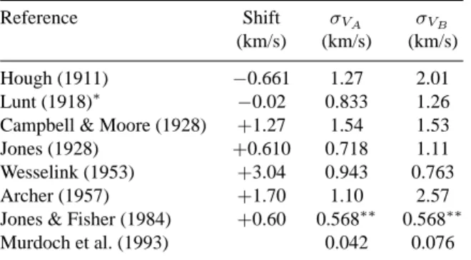
Table 1. Shift and standard deviations for each group of radial veloci-ties. Reference Shift σVA σVB (km/s) (km/s) (km/s) Hough (1911) −0.661 1.27 2.01 Lunt (1918)∗ −0.02 0.833 1.26
Campbell & Moore (1928) +1.27 1.54 1.53
Jones (1928) +0.610 0.718 1.11
Wesselink (1953) +3.04 0.943 0.763
Archer (1957) +1.70 1.10 2.57
Jones & Fisher (1984) +0.60 0.568∗∗ 0.568∗∗
Murdoch et al. (1993) 0.042 0.076
∗Wright’s (1904) measurements are not included.
∗∗Since there is only one observation, theseσ are just the residuals. Here are the sources of radial velocities coupled to the data after Murdoch et al. (1993) to compose the most extended radial velocity set:
– Hough (1911) and Jones (1928) published two sets of radial
velocities taken at the Cape Observatory in 1904–1908 and 1908–1924.
– Lunt (1918) took some spectra between 1904 and 1912. – Campbell & Moore (1928) compiled the radial velocities
obtained at Santiago between 1904 and 1922. The authors gave empirical corrections to apply to individual measure-ments depending on who obtained them, where and when.
– Wesselink (1953) took some spectra around the extrema of
the radial velocities. Unfortunately, although the epoch of the extrema had been known for a long time (Jones, 1928), very few spectra were taken at that epoch.
– Archer (1957) obtained some points in the steepest part of
the radial velocity curves, just after the extrema.
– Jones & Fisher (1984) determined just one radial velocity
of each component in 1972, almost coincident with the sec-ondary extrema.
The shift applied to each set as well as the standard deviations of the radial velocities within each group are summarized in Table 1.
Each term of the objective function (Pourbaix, 1998) incor-porates the weight associated to the observation. Although one may have a different weight for each observation, we assign the same weight to a group of observations. The weight of such a group is given by the inverse of the standard deviation of the members of the group. We thus adopt the values of Table 1 (Columns 3 and 4) for the radial velocities. We also set differ-ent weights for the polar and Cartesian observations. There is no need for relative weights of the radial velocities with respect to the astrometric data (Eq. 17 in (Pourbaix, 1998))
The orbit we derive is given in Table 2 and plotted in Fig. 1. We notice upward revisions of the distance and masses (6% and 7% for A and B respectively with respect to the estimates of Kamper & Wesselink (1978)). The new mass ratio is fully consistent with the astrometric one by Kamper & Wesselink (1978). We have thus obtained the first agreement between the
Spectroscopic orbit
Radial velocity (km/s)
Time
1904.14 1991.61 -35.0 -15.0Visual orbit
x (")
y (")
-30.00 15.00 15.00 -30.00Fig. 1. Plot of the orbit corresponding to the best adjustment of all visual and spectroscopic data. The radial velocities of component B are represented with open squares. The radial velocities of Murdoch et al. (1993) are those after 1988
astrometric and spectroscopic mass ratios. The orbital parallax is discrepant with all previous estimates, the Hipparcos one being the closest to ours.
Our estimates ofa and i are very close to those of Heintz (1958). The noticed reduction of the parallax and the corre-sponding increase of the masses are therefore due to an increase
Table 2. Orbital parameters and their standard deviations ofα Cen after the simultaneous adjustment of all visual observations and the radial velocities
Element Value Std. dev.
a (00) 17.59 0.028 i (◦) 79.23 0.046 ω (◦) 231.8 0.15 Ω (◦) 204.82 0.087 e 0.519 0.0013 P (yr) 79.90 0.013 T (Besselian year) 1955.59 0.019 V0(km/s) −21.87 0.054 $ (mas) 737.0 2.6 κ 0.45 0.013 mass A (M ) 1.16 0.031 mass B (M ) 0.97 0.032
of at least one radial velocity amplitude. There is nothing puz-zling with that since our spectroscopic orbit is one of the first one which takes all spectroscopic observations into account.
4. Evolutionary models ofα Cen A and B
What are the consequences of these new masses? Does it remove the discrepancies noted by Popper (1997) when the fit of an isochrone is undertaken?
Two theoretical evolutionary models have been computed with the assumption that the two stars have a common ori-gin, i.e. the same age and the same chemical composition. For a given stellar mass (MA or MB), a theoretical model of α Cen A or B contains the following parameters: the age t of the system, its initial hydrogen contentX, its initial metallic-ity Z and the convection parameter (αA or αB), when con-vection is treated in the mixing length approximation. These parameters have to be adjusted so that the models reproduce the available observables within their error bars. Such mod-els are referred to as calibrated modmod-els. The observables con-straining the models are: the visual apparent magnitudesmv,A= −0.01± 0.005, mv,b= 1.33± 0.005 (Hoffleit & Jaschek, 1982), the effective temperatures T eA = 5830 ± 30 K, T eB = 5255± 50 K (Neuforge-Verheecke & Magain, 1997), the sur-face gravities log gA = 4.34 ± 0.05, log gB = 4.51 ± 0.08 (Neuforge-Verheecke & Magain, 1997) and the logarith-mic abundance ratio of heavy elements to hydrogen, relative to the corresponding ratio for the Sun, [Z/X] = 0.25 ± 0.06 (Neuforge-Verheecke & Magain, 1997).
Our models are calculated with the Li`ege stellar evolution code based on a first version originally developed by Henyey et al. (1964). The Debye-Huckel corrections (Noels et al., 1984) are included in the equation of state of Bodenheimer et al. (1965), the nuclear reaction rates are those of Fowler et al. (1975), the treatment of the photospheric layers is taken from Krishna-Swamy (1969). The interior opacities are OPAL opac-ities taken from Iglesias & Rogers (1996), the low-T opacities
(T≤ 104K) are from Neuforge (1993) and the bolometric
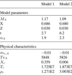
cor-Table 3. Model parameters (mass, initial hydrogen content, initial metallicity, age and convection parameter) and physical characteristics (visual magnitude, effective temperatureT e (in K), central hydrogen contentXc, central temperatureTc(in K) and central densityρc(in
g/cm3)) of the calibrated models ofα Cen A. Model 1 Model 2 Model parameters MA 1.17 1.09 X 0.686 0.680 Z 0.030 0.030 t 2.7 6.2 αA 1.9 2.3 Physical characteristics mv,A −0.01 −0.01 T eA 5848 5826 Xc 0.359 0.006 Tc 1.725E7 1.873E7 ρc 1.271E2 3.003E2
rections are from Flower (1996). Our models do not include diffusion and settling.
ForMA= 1.17M andMB= 0.96M , the observables are reproduced with the following model parameters:X = 0.686 ± 0.054,Z = 0.030 ± 0.004, t = 2.7 Gyr, αA= 1.86± 0.80, αB = 2.1± 0.80. The error bars on the model parameters result from the uncertainties affecting all the observables, including the masses (see (Brown et al., 1994) for the details of the calcu-lations). These uncertainties are huge on the age and have not been quoted here. This means that the age is not very well con-strained by the observations. The parameters and the physical characteristics of ourα Cen A model, chosen at the center of the error bars, are presented in Table 3. Table 3 also shows the char-acteristics of a previous model (Model 2) calculated with the same input physics and obeying to the same observational con-straints except for the orbital parameters, which have been taken from Kamper & Wesselink (1978), Heintz (1982) and Demar-que et al. (1986). Bothα Cen A models lie in the main-sequence band: they are burning hydrogen in their central layers, although Model 2 is very close to the end of the main sequence. Model 1 has a small convective core as a result of its higher mass. The problem in isochrone fitting (Popper, 1997), which was prob-ably due to the use of a fixed chemical composition, has been removed here. The comparison between the models and the ob-servational results may seem to be a never ending quest, since the models are continuously being improved and the error bars on the observations allow most of the time satisfactory models to be found. The hope is that asteroseismology will bring ad-ditional constraints which will be able to reduce the number of possible models (Brown et al., 1994).
We also computed the p-mode oscillation frequencies in both models for l = 0, 1, 2, 3 and for 1300 µHz ≤ νnl ≤ 3300µHz. Although no ambiguous detection has been reported yet, oscillation data of low degree might nevertheless soon be
100 105 110 115 120 1200 1400 1600 1800 2000 2200 2400 2600 2800 3000 3200 3400
Large frequency separation
frequency l=0 modele 1 modele 2 100 105 110 115 120 1400 1600 1800 2000 2200 2400 2600 2800 3000 3200 3400 frequency l=1 modele 1 modele 2
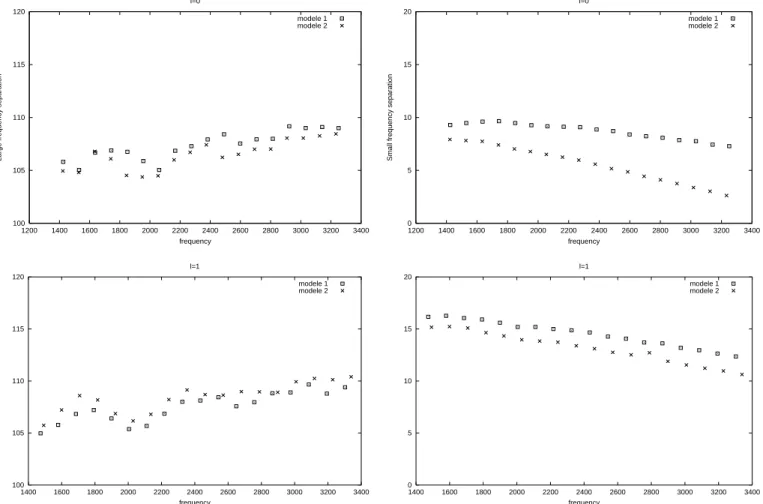
Fig. 2. ∆ν (l=0) as a function of ν (in µHz) for Model 1 (squares) and Model 2 (crosses). The top panel is for l=0 and the bottom one for l=1
obtained for α Cen A (Kjeldsen & Bedding, 1997). We com-puted the large and the small p-mode frequency separations,
∆νn,l = νn,l− νn−1,landδνn,l = νn,l− νn−1,l+2.ν is the frequency of the p-mode andn, l are respectively its order and its degree.∆ν is an indicator of the mean density of the star. δν decreases as the star evolves and gives clues to its evolutionary status.∆νn,landδνn,lare given as functions ofν in Figs. 2 and 3, for l=0 and l=1.
Model 1 is more massive and therefore younger and less evolved than Model 2 as indicated by its higher central hy-drogen content and its small frequency separations. The small frequency separations of this model differ from those of Model 2 by amounts much larger than the expected observational er-ror bars (' 1 µHz, (Brown et al., 1994)). The two models could thus be discriminated. If asteroseismology favors the lower mass model, could the mass difference be explained by the presence of a planet?
5. On the possibility of a planet aroundα Cen A or B
In the previous sections, we assumed that the mass we obtain for components A and B are the masses of stars A and B. Actually, one cannot reject the possibility for component A (or B) of being
0 5 10 15 20 1200 1400 1600 1800 2000 2200 2400 2600 2800 3000 3200 3400
Small frequency separation
frequency l=0 modele 1 modele 2 0 5 10 15 20 1400 1600 1800 2000 2200 2400 2600 2800 3000 3200 3400 frequency l=1 modele 1 modele 2
Fig. 3. δν (l=0) as a function of ν (in µHz) for Model 1 (squares) and Model 2 (crosses). The top panel is for l=0 and the bottom one for l=1
star A (or B) plus an unseen companion. The more massive the companion, the lesser massive the star.
The question of the detection of a possible planet orbit-ing aroundα Cen A or B rose with the drastic improvement of the spectroscopy. Dynamical simulations show that a planet could remain bound (Benest, 1988; Wiegert & Holman, 1997) but no spectroscopic campaign has revealed such a companion (Murdoch et al., 1993; Hatzes et al., 1996).
What would be the effect of a planet on the radial veloc-ity ofα Cen A? If one assumes 10−2M for the mass of the planet (ten times the mass of Jupiter), 3 A.U. for the semi-major axis of the orbit (the upper bound for a stable circular orbit (Wiegert & Holman, 1997)) and co-planar orbits, we obtain an amplitude of 136 m/s. Such an amplitude is reachable with the most up to date spectroscopic techniques. Therefore, it is very unlikely that even one percent of the mass ofα Cen A comes from a planet.
6. Conclusions
Current visual and spectroscopic observations yield component masses larger than previous estimates. Further observations, es-pecially very accurate radial velocities, are needed to confirm
those results. We urge southern spectroscopists to put a high priority onα Cen.
Acknowledgements. We thank R.E. Wilson for his careful reading of
the manuscript and his valuable suggestions. We also thank C.E. Worley for supplying the visual observations and D.M. Popper, the referee, for providing us with useful comments.
References
Archer S., 1957, MNRAS 117, 641 Benest D., 1988, A&A 206, 1143
Bodenheimer P., Forbes J., Gould N., Henyey L., 1965, ApJ 141, 1019 Brown T., Christensen-Dalsgaard J., Weibel-Mihalas B., Gilliland R.,
1994, ApJ 427(2), 1013
Campbell W., Moore J., 1928, Publ. of the Lick Observatory 16, 1 Demarque P., Guenther D., Van Althena W., 1986, ApJ 300, 773 ESA, 1997, The Hipparcos and Tycho Catalogues. ESA SP-1200 Flower P., 1996, ApJ 469, 355
Fowler W., Coughlan G., Zimmerman B., 1975, ARA&A 13, 69 Hatzes A., K¨urster M., Cochran W., Dennerl K., D¨obereiner S., 1996,
Journal of Geophysical Research E 101, 9285 Heintz W., 1958, Ver¨off. M¨unch 5, 100
Heintz W., 1982, Observatory 102, 42
Henyey L., Forbes J., Gould N., 1964, ApJ 139, 306
Hoffleit D., Jaschek C., 1982, Bright Star Catalogue. Yale University Observatory, New Haven, 4 edition
Hough S., 1911, Annals of the Cape Observatory 10(1), 1 Iglesias C., Rogers F., 1996, ApJ 464, 943
Jones D., Fisher J., 1984, A&AS 56, 449
Jones H., 1928, Annals of the Cape Observatory 10(8), 95 Kamper K., Wesselink A., 1978, AJ 83, 1653
Kjeldsen H., Bedding T., 1997, In: Bedding T., Booth A., Davis J. (eds.) Fundamental Stellar Properties: The Interaction between Observa-tion and Theory. Kluwer Academic Publishers
Krishna-Swamy K., 1969, ApJ 145, 74 Lunt J., 1918, ApJ 48, 182
Morbey C., 1975, PASP 87, 689
Murdoch K., Hearnshaw J., 1993, Observatory 113, 79 Murdoch K., Hearnshaw J., Clark M., 1993, ApJ 413, 349 Neuforge C., 1993, A&A 274, 818
Neuforge-Verheecke C., Magain P., 1997, A&A 328, 261
Neuforge-Verheecke C., Noels A., 1998, In: Bradley P., Guzik J. (eds.) A Half Century of Stellar Pulsations Interpretations: a tribute to Arthur N. Cox. ASP Conference Series #135
Noels A., Scuflaire R., Gabriel M., 1984, A&A 130, 389 Popper D., 1997, AJ 114, 1195
Pourbaix D., 1998, A&AS 131, 377 Wesselink A., 1953, MNRAS 113, 505 Wiegert P. Holman M., 1997, AJ 113, 1445 Wright W., 1904, ApJ 20, 140