BlinkDB: queries with bounded errors and
bounded response times on very large data
The MIT Faculty has made this article openly available.
Please share
how this access benefits you. Your story matters.
Citation
Sameer Agarwal, Barzan Mozafari, Aurojit Panda, Henry Milner,
Samuel Madden, and Ion Stoica. 2013. BlinkDB: queries with
bounded errors and bounded response times on very large data.
In Proceedings of the 8th ACM European Conference on Computer
Systems (EuroSys '13). ACM, New York, NY, USA, 29-42.
As Published
http://dx.doi.org/10.1145/2465351.2465355
Publisher
Association for Computing Machinery (ACM)
Version
Author's final manuscript
Citable link
http://hdl.handle.net/1721.1/100911
Terms of Use
Creative Commons Attribution-Noncommercial-Share Alike
BlinkDB: Queries with Bounded Errors and
Bounded Response Times on Very Large Data
Sameer Agarwal
†, Barzan Mozafari
○, Aurojit Panda
†, Henry Milner
†, Samuel Madden
○, Ion Stoica
∗††University of California, Berkeley ○Massachusetts Institute of Technology ∗Conviva Inc.
{sameerag, apanda, henrym, istoica}@cs.berkeley.edu, {barzan, madden}@csail.mit.edu
Abstract
In this paper, we presentBlinkDB, a massively parallel,
ap-proximate query engine for running interactive SQL queries
on large volumes of data. BlinkDB allows users to
trade-off query accuracy for response time, enabling interactive queries over massive data by running queries on data samples and presenting results annotated with meaningful error bars. To achieve this,BlinkDBuses two key ideas:(1) an adaptive
optimization framework that builds and maintains a set of multi-dimensional stratified samples from original data over time, and(2) a dynamic sample selection strategy that selects an appropriately sized sample based on a query’s accuracy or response time requirements. We evaluateBlinkDBagainst the
well-known TPC-H benchmarks and a real-world analytic workload derived from Conviva Inc., a company that man-ages video distribution over the Internet. Our experiments on a 100 node cluster show thatBlinkDBcan answer queries
on up to 17 TBs of data in less than 2 seconds (over 200× faster than Hive), within an error of 2-10%.
1.
Introduction
Modern data analytics applications involve computing aggre-gates over a large number of records to roll-up web clicks, online transactions, content downloads, and other features along a variety of different dimensions, including demo-graphics, content type, region, and so on. Traditionally, such queries have been executed using sequential scans over a large fraction of a database. Increasingly, new applications demand near real-time response rates. Examples may include applications that (i) update ads on a website based on trends in social networks like Facebook and Twitter, or (ii) deter-mine the subset of users experiencing poor performance based on their service provider and/or geographic location. Over the past two decades a large number of approxima-tion techniques have been proposed, which allow for fast
pro-Permission to make digital or hard copies of all or part of this work for personal or classroom use is granted without fee provided that copies are not made or distributed for profit or commercial advantage and that copies bear this notice and the full citation on the first page. To copy otherwise, to republish, to post on servers or to redistribute to lists, requires prior specific permission and/or a fee.
Eurosys’13 April 15-17, 2013, Prague, Czech Republic Copyright © 2013 ACM 978-1-4503-1994-2/13/04. . . $15.00
cessing of large amounts of data by trading result accuracy for response time and space. These techniques include sam-pling [10,14], sketches [12], and on-line aggregation [15]. To illustrate the utility of such techniques, consider the following simple query that computes the average SessionTime over all users originating in New York:
SELECT AVG(SessionTime) FROM Sessions
WHERE City = ‘New York’
Suppose the Sessions table contains 100 million tuples for New York, and cannot fit in memory. In that case, the above query may take a long time to execute, since disk reads are ex-pensive, and such a query would need multiple disk accesses to stream through all the tuples. Suppose we instead exe-cuted the same query on a sample containing only 10, 000 New York tuples, such that the entire sample fits in mem-ory. This would be orders of magnitude faster, while still pro-viding an approximate result within a few percent of the ac-tual value, an accuracy good enough for many practical pur-poses. Using sampling theory we could even provide confi-dence bounds on the accuracy of the answer [16].
Previously described approximation techniques make dif-ferent trade-offs between efficiency and the generality of the queries they support. At one end of the spectrum, exist-ing samplexist-ing and sketch based solutions exhibit low space and time complexity, but typically make strong assumptions about the query workload (e.g., they assume they know the set of tuples accessed by future queries and aggregation func-tions used in queries). As an example, if we know all future queries are on large cities, we could simply maintain random samples that omit data about smaller cities.
At the other end of the spectrum, systems like online
aggregation (OLA) [15] make fewer assumptions about the
query workload, at the expense of highly variable perfor-mance. Using OLA, the above query will likely finish much faster for sessions in New York (i.e., the user might be satisfied with the result accuracy, once the query sees the first 10, 000 sessions from New York) than for sessions in Galena, IL, a town with fewer than 4, 000 people. In fact, for such a small town, OLA may need to read the entire table to compute a result with satisfactory error bounds.
In this paper, we argue that none of the previous solutions are a good fit for today’s big data analytics workloads. OLA
provides relatively poor performance for queries on rare tu-ples, while sampling and sketches make strong assumptions about the predictability of workloads or substantially limit the types of queries they can execute.
To this end, we proposeBlinkDB, a distributed
sampling-based approximate query processing system that strives to achieve a better balance between efficiency and generality for analytics workloads.BlinkDBallows users to pose SQL-based
aggregation queries over stored data, along with response time or error bound constraints. As a result, queries over mul-tiple terabytes of data can be answered in seconds, accom-panied by meaningful error bounds relative to the answer that would be obtained if the query ran on the full data. In contrast to most existing approximate query solutions (e.g., [10]),BlinkDBsupports more general queries as it makes no
assumptions about the attribute values in the WHERE, GROUP BY, and HAVING clauses, or the distribution of the values used by aggregation functions. Instead,BlinkDBonly assumes that
the sets of columns used by queries in WHERE, GROUP BY, and HAVING clauses are stable over time. We call these sets of columns “query column sets” orQCSs in this paper.
BlinkDBconsists of two main modules: (i) Sample
Cre-ation and (ii) Sample Selection. The sample creCre-ation module creates stratified samples on the most frequently usedQCSs to
ensure efficient execution for queries on rare values. By strat-ified, we mean that rare subgroups (e.g., Galena, IL) are over-represented relative to a uniformly random sample. This ensures that we can answer queries about any subgroup, re-gardless of its representation in the underlying data.
We formulate the problem of sample creation as an opti-mization problem. Given a collection of pastQCSand their
historical frequencies, we choose a collection of stratified samples with total storage costs below some user configurable storage threshold. These samples are designed to efficiently answer queries with the sameQCSs as past queries, and to
provide good coverage for future queries over similarQCS.
If the distribution ofQCSs is stable over time, our approach
creates samples that are neither over- nor under-specialized for the query workload. We show that in real-world work-loads from Facebook Inc. and Conviva Inc.,QCSs do re-occur
frequently and that stratified samples built using historical
patterns ofQCSusage continue to perform well for future
queries. This is in contrast to previous optimization-based sampling systems that assume complete knowledge of the tu-ples accessed by queries at optimization time.
Based on a query’s error/response time constraints, the sample selection module dynamically picks a sample on which to run the query. It does so by running the query on multiple smaller sub-samples (which could potentially be stratified across a range of dimensions) to quickly estimate query selectivity and choosing the best sample to satisfy spec-ified response time and error bounds. It uses an Error-Latency Profileheuristic to efficiently choose the sample that will best satisfy the user-specified error or time bounds.
We implementedBlinkDB1 on top of Hive/Hadoop [22]
(as well as Shark [13], an optimized Hive/Hadoop framework that caches input/ intermediate data). Our implementation requires minimal changes to the underlying query processing system. We validate its effectiveness on a 100 node cluster, us-ing both the TPC-H benchmarks and a real-world workload
derived from Conviva. Our experiments show thatBlinkDB
can answer a range of queries within 2 seconds on 17 TB of data within 90-98% accuracy, which is two orders of magni-tude faster than running the same queries on Hive/Hadoop. In summary, we make the following contributions:
• We use a column-set based optimization framework to
compute a set of stratified samples (in contrast to ap-proaches like AQUA [6] and STRAT [10], which compute only a single sample per table). Our optimization takes into account: (i) the frequency of rare subgroups in the data, (ii) the column sets in the past queries, and (iii) the storage overhead of each sample. (§4)
• We create error-latency profiles (ELPs) for each query at runtime to estimate its error or response time on each available sample. This heuristic is then used to select the most appropriate sample to meet the query’s response time or accuracy requirements. (§5)
• We show how to integrate our approach into an existing parallel query processing framework (Hive) with minimal changes. We demonstrate that by combining these ideas together,BlinkDBprovides bounded error and latency for
a wide range of real-world SQL queries, and it is robust to variations in the query workload. (§6)
2.
Background
Any sampling based query processor, including BlinkDB,
must decide what types of samples to create. The sample cre-ation process must make some assumptions about the nature of the future query workload. One common assumption is that future queries will be similar to historical queries. While this assumption is broadly justified, it is necessary to be pre-cise about the meaning of “similarity” when building a work-load model. A model that assumes the wrong kind of sim-ilarity will lead to a system that “over-fits” to past queries and produces samples that are ineffective at handling future workloads. This choice of model of past workloads is one of the key differences betweenBlinkDBand prior work. In the
rest of this section, we present a taxonomy of workload mod-els, discuss our approach, and show that it is reasonable using experimental evidence from a production system.
2.1 Workload Taxonomy
Offline sample creation, caching, and virtually any other type of database optimization assumes a target workload that can be used to predict future queries. Such a model can either be trained on past data, or based on information provided by
1
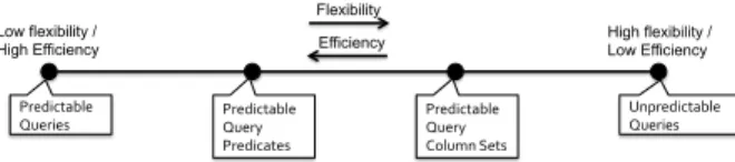
users. This can range from an ad-hoc model, which makes no assumptions about future queries, to a model which assumes that all future queries are known a priori. As shown in Fig.1, we classify possible approaches into one of four categories:
Flexibility Efficiency Low flexibility /
High Efficiency High flexibility / Low Efficiency
Predictable
Queries Predictable Query Predicates Predictable Query Column Sets Unpredictable Queries
Figure 1. Taxonomy of workload models.
1. Predictable Queries: At the most restrictive end of the spectrum, one can assume that all future queries are known in advance, and use data structures specially designed for these queries. Traditional databases use such a model for lossless synopsis [12] which can provide extremely fast responses for certain queries, but cannot be used for any other queries. Prior work in approximate databases has also proposed using lossy sketches (including wavelets and histograms) [14].
2. Predictable Query Predicates: A slightly more flexi-ble model is one that assumes that the frequencies of group and filter predicates — both the columns and the values in WHERE, GROUP BY, and HAVING clauses — do not change over time. For example, if 5% of past queries include only the filter WHERE City = ‘New York’ and no other group or filter predicates, then this model predicts that 5% of future queries will also include only this filter. Under this model, it is possible to predict future filter predicates by observing a prior workload. This model is employed by materialized views in traditional databases. Approximate databases, such as STRAT [10] and SciBORQ [21], have similarly relied on prior queries to determine the tuples that are likely to be used in future queries, and to create samples containing them.
3. Predictable QCSs: Even greater flexibility is provided by assuming a model where the frequency of the sets of columns used for grouping and filtering does not change over time, but the exact values that are of interest in those columns are unpredictable. We term the columns used for grouping and filtering in a query the query column set, orQCS, for the
query. For example, if 5% of prior queries grouped or filtered
on theQCS{City}, this model assumes that 5% of future
queries will also group or filter on thisQCS, though the
par-ticular predicate may vary. This model can be used to decide the columns on which building indices would optimize data access. Prior work [20] has shown that a similar model can be used to improve caching performance in OLAP systems.
AQUA [4], an approximate query database based on
sam-pling, uses theQCSmodel. (See §8for a comparison between
AQUA andBlinkDB).
4. Unpredictable Queries: Finally, the most general model assumes that queries are unpredictable. Given this as-sumption, traditional databases can do little more than just rely on query optimizers which operate at the level of a single query. In approximate databases, this workload model does
not lend itself to any “intelligent” sampling, leaving one with no choice but to uniformly sample data. This model is used by On-Line Aggregation (OLA) [15], which relies on streaming data in random order.
While the unpredictable query model is the most flexible one, it provides little opportunity for an approximate query processing system to efficiently sample the data. Further-more, prior work [11,19] has argued that OLA performance’s on large clusters (the environment on whichBlinkDBis
in-tended to run) falls short. In particular, accessing individual rows randomly imposes significant scheduling and commu-nication overheads, while accessing data at the HDFS block2 level may skew the results.
As a result, we use the model of predictableQCSs. As we
will show, this model provides enough information to enable efficient pre-computation of samples, and it leads to samples that generalize well to future workloads in our experiments. Intuitively, such a model also seems to fit in with the types of exploratory queries that are commonly executed on large scale analytical clusters. As an example, consider the oper-ator of a video site who wishes to understand what types of videos are popular in a given region. Such a study may require looking at data from thousands of videos and hun-dreds of geographic regions. While this study could result in a very large number of distinct queries, most will use only two columns, video title and viewer location, for grouping and filtering. Next, we present empirical evidence based on real world query traces from Facebook Inc. and Conviva Inc. to support our claims.
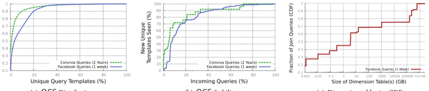
2.2 Query Patterns in a Production Cluster
To empirically test the validity of the predictableQCSmodel
we analyze a trace of 18, 096 queries from 30 days of queries from Conviva and a trace of 69, 438 queries constituting a random, but representative, fraction of 7 days’ workload from Facebook to determine the frequency ofQCSs.
Fig.2(a)shows the distribution ofQCSs across all queries
for both workloads. Surprisingly, over 90% of queries are cov-ered by 10% and 20% of uniqueQCSs in the traces from
Con-viva and Facebook respectively. Only 182 uniqueQCSs cover
all queries in the Conviva trace and 455 uniqueQCSs span all
the queries in the Facebook trace. Furthermore, if we remove theQCSs that appear in less than 10 queries, we end up with
only 108 and 211QCSs covering 17, 437 queries and 68, 785
queries from Conviva and Facebook workloads, respectively. This suggests that, for real-world production workloads,
QCSs represent an excellent model of future queries.
Fig. 2(b)shows the number of unique QCSs versus the
queries arriving in the system. We define uniqueQCSs as
QCSs that appear in more than 10 queries. For the
Con-viva trace, after only 6% of queries we already see close to 60% of allQCSs, and after 30% of queries have arrived, we
see almost allQCSs — 100 out of 108. Similarly, for the
0.1 0.2 0.3 0.4 0.5 0.6 0.7 0.8 0.9 1 0 20 40 60 80 100 Fracti on of Queri es (CD F)
Unique Query Templates (%) Conviva Queries (2 Years) Facebook Queries (1 week)
(a)QCSDistribution 0 10 20 30 40 50 60 70 80 90 100 0 20 40 60 80 100 Ne w Uni que Tem plates Seen (%) Incoming Queries (%) Conviva Queries (2 Years) Facebook Queries (1 week)
(b)QCSStability 0.1 0.2 0.3 0.4 0.5 0.6 0.7 0.8 0.9 1 0.001 0.01 0.1 1 10 100 1000 10000 100000 1e+06
Fraction of Join Queries (CDF)
Size of Dimension Table(s) (GB)
Facebook Queries (1 Week)
(c) Dimension table size CDF
Figure 2. 2(a)and2(b)show the distribution and stability ofQCSs respectively across all queries in the Conviva and
Face-book traces.2(c)shows the distribution of join queries with respect to the size of dimension tables. book trace, after 12% of queries, we see close to 60% of all
QCSs, and after only 40% queries, we see almost allQCSs —
190 out of 211. This shows thatQCSs are relatively stable over
time, which suggests that the past history is a good predictor for the future workload.
3.
System Overview
Sample'Selection' TABLE' Distributed' Cache' Distributed' Filesystem' Original'' Data' Shark' ' SELECT COUNT(*)! FROM TABLE! WHERE (city=“NY”)! LIMIT 1s;! HiveQL/SQL' Query' Result:( 1,101,822(±(2,105&& (95%(confidence)( Sa m pl e' Cre at io n' & ' Main ten an ce'Figure 3. BlinkDBarchitecture.
Fig.3shows the overall architecture ofBlinkDB.BlinkDB
extends the Apache Hive framework [22] by adding two ma-jor components to it: (1) an offline sampling module that cre-ates and maintains samples over time, and (2) a run-time sample selection module that creates an Error-Latency Pro-file (ELP)for queries. To decide on the samples to create, we use theQCSs that appear in queries (we present a more
pre-cise formulation of this mechanism in §4.) Once this choice is made, we rely on distributed reservoir sampling3[23] or bi-nomial sampling techniques to create a range of uniform and stratified samples across a number of dimensions.
At run-time, we employ ELP to decide the sample to run the query. The ELP characterizes the rate at which the error (or response time) decreases (or increases) as the size of the sample on which the query operates increases. This is used to select a sample that best satisfies the user’s constraints. We describe ELP in detail in §5.BlinkDBalso augments the query
parser, optimizer, and a number of aggregation operators to allow queries to specify bounds on error, or execution time.
3Reservoir sampling is a family of randomized algorithms for creating
fixed-sized random samples from streaming data.
3.1 Supported Queries
BlinkDB supports a slightly constrained set of SQL-style
declarative queries, imposing constraints that are similar to prior work [10]. In particular,BlinkDBcan currently provide
approximate results for standard SQL aggregate queries in-volving COUNT, AVG, SUM and QUANTILE. Queries involv-ing these operations can be annotated with either an error bound, or a time constraint. Based on these constraints, the system selects an appropriate sample, of an appropriate size, as explained in §5.
As an example, let us consider querying a table Sessions, with five columns, SessionID, Genre, OS, City, and URL, to determine the number of sessions in which users viewed content in the “western” genre, grouped by OS. The query:
SELECT COUNT(*) FROM Sessions
WHERE Genre = ‘western’ GROUP BY OS
ERROR WITHIN 10% AT CONFIDENCE 95%
will return the count for each GROUP BY key, with each count
having relative error of at most±10% at a 95% confidence
level. Alternatively, a query of the form:
SELECT COUNT(*) FROM Sessions
WHERE Genre = ‘western’ GROUP BY OS
WITHIN 5 SECONDS
will return the most accurate results for each GROUP BY key in 5 seconds, along with a 95% confidence interval for the relative error of each result.
WhileBlinkDBdoes not currently support arbitrary joins
and nested SQL queries, we find that this is usually not a hin-drance. This is because any query involving nested queries or joins can be flattened to run on the underlying data. How-ever, we do provide support for joins in some settings which are commonly used in distributed data warehouses. In par-ticular,BlinkDB can support joining a large, sampled fact
table, with smaller tables that are small enough to fit in the main memory of any single node in the cluster. This is one
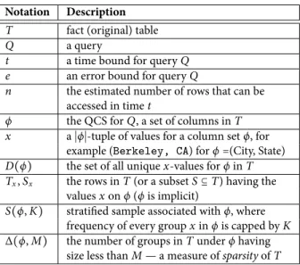
Notation Description
T fact (original) table Q a query
t a time bound for query Q e an error bound for query Q
n the estimated number of rows that can be accessed in time t
ϕ the QCS for Q, a set of columns in T x a ∣ϕ∣-tuple of values for a column set ϕ, for
example (Berkeley, CA) for ϕ =(City, State) D(ϕ) the set of all unique x-values for ϕ in T Tx, Sx the rows in T (or a subset S ⊆ T) having the
values x on ϕ (ϕ is implicit)
S(ϕ, K) stratified sample associated with ϕ, where frequency of every group x in ϕ is capped by K ∆(ϕ, M) the number of groups in T under ϕ having
size less than M — a measure of sparsity of T
Table 1. Notation in §4.1
of the most commonly used form of joins in distributed data warehouses. For instance, Fig.2(c)shows the distribution of the size of dimension tables (i.e., all tables except the largest) across all queries in a week’s trace from Facebook. We ob-serve that 70% of the queries involve dimension tables that are less than 100 GB in size. These dimension tables can be easily cached in the cluster memory, assuming a cluster consisting of hundreds or thousands of nodes, where each node has at least 32 GB RAM. It would also be straightforward to extend
BlinkDBto deal with foreign key joins between two sampled
tables (or a self join on one sampled table) where both ta-bles have a stratified sample on the set of columns used for joins. We are also working on extending our query model to support more general queries, specifically focusing on more complicated user defined functions, and on nested queries.
4.
Sample Creation
BlinkDBcreates a set of samples to accurately and quickly
an-swer queries. In this section, we describe the sample creation process in detail. First, in §4.1, we discuss the creation of a stratified sample on a given set of columns. We show how a query’s accuracy and response time depends on the availabil-ity of stratified samples for that query, and evaluate the stor-age requirements of our stratified sampling strategy for vari-ous data distributions. Stratified samples are useful, but carry storage costs, so we can only build a limited number of them. In §4.2we formulate and solve an optimization problem to decide on the sets of columns on which we build samples.
4.1 Stratified Samples
In this section, we describe our techniques for constructing a sample to target queries using a given QCS. Table1contains the notation used in the rest of this section.
Queries that do not filter or group data (for example, a SUM over an entire table) often produce accurate answers when run on uniform samples. However, uniform sampling often
does not work well for a queries on filtered or grouped subsets of the table. When members of a particular subset are rare, a larger sample will be required to produce high-confidence estimates on that subset. A uniform sample may not contain any members of the subset at all, leading to a missing row in the final output of the query. The standard approach to solv-ing this problem is stratified samplsolv-ing [16], which ensures that rare subgroups are sufficiently represented. Next, we describe the use of stratified sampling inBlinkDB.
4.1.1 Optimizing a stratified sample for a single query
First, consider the smaller problem of optimizing a stratified sample for a single query. We are given a query Q specifying a table T, a QCS ϕ, and either a response time bound t or an error bound e. A time bound t determines the maximum sample size on which we can operate, n; n is also the opti-mal sample size, since larger samples produce better statisti-cal results. Similarly, given an error bound e, it is possible to calculate the minimum sample size that will satisfy the error bound, and any larger sample would be suboptimal because it would take longer than necessary. In general n is monoton-ically increasing in t (or monotonmonoton-ically decreasing in e) but will also depend on Q and on the resources available in the cluster to process Q. We will show later in §5how we estimate nat runtime using an Error-Latency Profile.
Among the rows in T, let D(ϕ) be the set of unique values xon the columns in ϕ. For each value x there is a set of rows in T having that value, Tx = {r ∶ r ∈ T and r takes values x on columns ϕ}. We will say that there are ∣D(ϕ)∣ “groups” Tx of rows in T under ϕ. We would like to compute an aggregate value for each Tx(for example, a SUM). Since that is expensive,
instead we will choose a sample S ⊆ T with ∣S∣ = n rows.
For each group Tx there is a corresponding sample group
Sx ⊆ S that is a subset of Tx, which will be used instead of Tx to calculate an aggregate. The aggregate calculation for each Sx will be subject to error that will depend on its size. The best sampling strategy will minimize some measure of the expected error of the aggregate across all the Sx, such as the worst expected error or the average expected error.
A standard approach is uniform sampling — sampling n rows from T with equal probability. It is important to un-derstand why this is an imperfect solution for queries that compute aggregates on groups. A uniform random sample allocates a random number of rows to each group. The size of sample group Sxhas a hypergeometric distribution with n draws, population size∣T∣, and ∣Tx∣ possibilities for the group to be drawn. The expected size of Sxis n
∣Tx∣
∣T ∣, which is propor-tional to∣Tx∣. For small ∣Tx∣, there is a chance that ∣Sx∣ is very small or even zero, so the uniform sampling scheme can miss some groups just by chance. There are 2 things going wrong: 1. The sample size assigned to a group depends on its size in T. If we care about the error of each aggregate equally, it is not clear why we should assign more samples to Sxjust because∣Tx∣ is larger.
2. Choosing sample sizes at random introduces the possibil-ity of missing or severely under-representing groups. The probability of missing a large group is vanishingly small, but the probability of missing a small group is substantial. This problem has been studied before. Briefly, since error decreases at a decreasing rate as sample size increases, the best choice simply assigns equal sample size to each groups. In addition, the assignment of sample sizes is deterministic, not random. A detailed proof is given by Acharya et al. [4]. This leads to the following algorithm for sample selection:
1. Compute group counts: To each x ∈
x0, ..., x∣D(ϕ)∣−1, assign a count, forming a
∣D(ϕ)∣-vector of counts N∗ n. Compute N ∗ n as follows: Let N(n′) = (min(⌊ n′ ∣D(ϕ)∣⌋, ∣Tx0∣), min(⌊ n′ ∣D(ϕ)∣⌋, ∣Tx1∣, ...), the optimal count-vector for a total sample size n′. Then choose N∗
n = N(max{n
′ ∶ ∣∣N(n′)∣∣
1 ≤ n}). In words, our
samples cap the count of each group at some value⌊ n′
∣D(ϕ)∣⌋. In the future we will use the name K for the cap size⌊ n′
∣D(ϕ)∣⌋. 2. Take samples: For each x, sample N∗
n xrows uniformly at random without replacement from Tx, forming the sample Sx. Note that when∣Tx∣ = N∗
n x, our sample includes all the rows of Tx, and there will be no sampling error for that group.
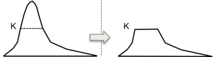
V(φ) S(φ)
K K
φ
Figure 4. Example of a stratified sample associated with a set
of columns, ϕ.
The entire sample S(ϕ, K) is the disjoint union of the Sx. Since a stratified sample on ϕ is completely determined by the group-size cap K, we henceforth denote a sample by S(ϕ, K) or simply S when there is no ambiguity. K determines the size and therefore the statistical properties of a stratified sample for each group.
For example, consider query Q grouping byQCSϕ, and
assume we use S(ϕ, K) to answer Q. For each value x on ϕ, if∣Tx∣ ≤ K, the sample contains all rows from the original table, so we can provide an exact answer for this group. On the other hand, if∣Tx∣ > K, we answer Q based on K random rows in the original table. For the basic aggregate operators AVG, SUM, COUNT, and QUANTILE, K directly determines the error of Q’s result. In particular, these aggregate operators have standard error inversely proportional to√K[16].
4.1.2 Optimizing a set of stratified samples for all queries sharing aQCS
Now we turn to the question of creating samples for a set of queries that share aQCSϕbut have different values of n. Recall that n, the number of rows we read to satisfy a query, will vary according to user-specified error or time bounds. A WHERE query may also select only a subset of groups, which
allows the system to read more rows for each group that is actually selected. So in general we want access to a family of stratified samples(Sn), one for each possible value of n.
Fortunately, there is a simple method that requires main-taining only a single sample for the whole family(Sn). Ac-cording to our sampling strategy, for a single value of n, the size of the sample for each group is deterministic and is monotonically increasing in n. In addition, it is not nec-essary that the samples in the family be selected indepen-dently. So given any sample Snm a x, for any n ≤ nm a x there
is an Sn ⊆ Snm a x that is an optimal sample for n in the sense
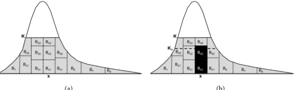
of the previous section. Our sample storage technique, de-scribed next, allows such subsets to be identified at runtime. The rows of stratified sample S(ϕ, K) are stored sequen-tially according to the order of columns in ϕ. Fig.5(a) shows an example of storage layout for S(ϕ, K). Bi jdenotes a data block in the underlying file system, e.g., HDFS. Records cor-responding to consecutive values in ϕ are stored in the same block, e.g., B1. If the records corresponding to a popular value do not all fit in one block, they are spread across several contiguous blocks e.g., blocks B41, B42and B43contain rows from Sx. Storing consecutive records contiguously on the disk significantly improves the execution times or range of the queries on the set of columns ϕ.
When Sx is spread over multiple blocks, each block
con-tains a randomly ordered random subset from Sx, and, by
extension, from the original table. This makes it possible to efficiently run queries on smaller samples. Assume a query Q, that needs to read n rows in total to satisfy its error
bounds or time execution constraints. Let nx be the
num-ber of rows read from Sxto compute the answer. (Note nx ≤ max{K, ∣Tx∣} and ∑x ∈D(ϕ),x selected by Qnx = n.) Since the rows are distributed randomly among the blocks, it is enough for Q to read any subset of blocks comprising Sx, as long as these blocks contain at least nxrecords. Fig.5(b) shows an ex-ample where Q reads only blocks B41and B42, as these blocks contain enough records to compute the required answer.
Storage overhead. An important consideration is the
over-head of maintaining these samples, especially for heavy-tailed distributions with many rare groups. Consider a table with 1 billion tuples and a column set with a Zipf distribution with an exponent of 1.5. Then, it turns out that the storage required by sample S(ϕ, K) is only 2.4% of the original table for K= 104, 5.2% for K= 105, and 11.4% for K= 106.
These results are consistent with real-world data from Conviva Inc., where for K= 105, the overhead incurred for a sample on popular columns like city, customer, autonomous system number (ASN) is less than 10%.
4.2 Optimization Framework
We now describe the optimization framework to select sub-sets of columns on which to build sample families. Un-like prior work which focuses on single-column stratified samples [9] or on a single dimensional (i.e., multi-column) stratified sample [4],BlinkDBcreates several
multi-K B1 B21 B22 B31 B32 B33 B41 B42 B51 B52 B6 B7 B8 B43 x (a) K B1 B21 B22 B31 B32 B33 B51 B52 B6 B7 B8 B43 K1 B42 B41 x (b)
Figure 5. (a) Possible storage layout for stratified sample S(ϕ, K).
dimensional stratified samples. As described above, each stratified sample can potentially be used at runtime to im-prove query accuracy and latency, especially when the orig-inal table contains small groups for a particular column set. However, each stored sample has a storage cost equal to its size, and the number of potential samples is exponential in the number of columns. As a result, we need to be careful in choosing the set of column-sets on which to build strati-fied samples. We formulate the trade-off between storage cost and query accuracy/performance as an optimization prob-lem, described next.
4.2.1 Problem Formulation
The optimization problem takes three factors into account in determining the sets of columns on which stratified samples should be built: the “sparsity” of the data, workload character-istics, and the storage cost of samples.
Sparsity of the data. A stratified sample on ϕ is useful when
the original table T contains many small groups under ϕ. Consider a QCS ϕ in table T. Recall that D(ϕ) denotes the set of all distinct values on columns ϕ in rows of T. We define a “sparsity” function ∆(ϕ, M) as the number of groups whose size in T is less than some number M4:
∆(ϕ, M) = ∣{x ∈ D(ϕ) ∶ ∣Tx∣ < M}∣
Workload. A stratified sample is only useful when it is
bene-ficial to actual queries. Under our model for queries, a query has a QCS qjwith some (unknown) probability pj- that is, QCSs are drawn from a Multinomial(p1, p2, ...) distribution. The best estimate of pjis simply the frequency of queries with QCS qjin past queries.
Storage cost. Storage is the main constraint against
build-ing too many stratified samples, and against buildbuild-ing strat-ified samples on large column sets that produce too many groups. Therefore, we must compute the storage cost of po-tential samples and constrain total storage. To simplify the formulation, we assume a single value of K for all samples; a sample family ϕ either receives no samples or a full sam-ple with K elements of Txfor each x∈ D(ϕ). ∣S(ϕ, K)∣ is the storage cost (in rows) of building a stratified sample on a set of columns ϕ.
4Appropriate values for M will be discussed later in this section.
Alterna-tively, one could plug in different notions of sparsity of a distribution in our formulation.
Given these three factors defined above, we now introduce our optimization formulation. Let the overall storage capacity budget (again in rows) be C. Our goal is to select β column sets from among m possibleQCSs, say ϕi1,⋯, ϕiβ, which can
best answer our queries, while satisfying: β
∑
k=1∣S(ϕ
ik, K)∣ ≤ C
Specifically, inBlinkDB, we maximize the following mixed
integer linear program (MILP) in which j indexes over all queries and i indexes over all possible column sets:
G= ∑ j pj⋅ yj⋅ ∆(qj, M) (1) subject to m ∑ i =1∣S(ϕ i, K)∣ ⋅ zi ≤ C (2) and ∀ j ∶ yj≤ max i ∶ϕi⊆qj∪ i ∶ϕi⊃qj(z imin 1, ∣ D(ϕi)∣ ∣D(qj)∣) (3) where 0≤ yj≤ 1 and zi∈ {0, 1} are variables.
Here, ziis a binary variable determining whether a sample family should be built or not, i.e., when zi = 1, we build a sample family on ϕi; otherwise, when zi= 0, we do not.
The goal function (1) aims to maximize the weighted sum of the coverage of theQCSs of the queries, qj. If we create a stratified sample S(ϕi, K), the coverage of this sample for qj is defined as the probability that a given value x of columns qj is also present among the rows of S(ϕi, K). If ϕi⊇ qj, then qj is covered exactly, but ϕi ⊂ qjcan also be useful by partially covering qj. At runtime, if no stratified sample is available that exactly covers a theQCSfor a query, a partially-covering QCS
may be used instead. In particular, the uniform sample is a degenerate case with ϕi= ∅; it is useful for many queries but less useful than more targeted stratified samples.
Since the coverage probability is hard to compute in prac-tice, in this paper we approximate it by yj, which is deter-mined by constraint (3). The yjvalue is in[0, 1], with 0 mean-ing no coverage, and 1 meanmean-ing full coverage. The intuition behind (3) is that when we build a stratified sample on a subset of columns ϕi ⊆ qj, i.e. when zi = 1, we have par-tially covered qj, too. We compute this coverage as the ra-tio of the number of unique values between the two sets, i.e.,
∣D(ϕi)∣/∣D(qj)∣. When ϕi ⊂ qj, this ratio, and the true cov-erage value, is at most 1. When ϕi= qj, the number of unique values in ϕiand qjare the same, we are guaranteed to see all the unique values of qjin the stratified sample over ϕiand therefore the coverage will be 1. When ϕi ⊃ qj, the coverage is also 1, so we cap the ratio∣D(ϕi)∣/∣D(qj)∣ at 1.
Finally, we need to weigh the coverage of each set of columns by their importance: a set of columns qjis more im-portant to cover when: (i) it appears in more queries, which is represented by pj, or (ii) when there are more small groups under qj, which is represented by ∆(qj, M). Thus, the best solution is when we maximize the sum of pj⋅ yj⋅ ∆(qj, M) for all QCSs, as captured by our goal function (1).
The size of this optimization problem increases exponen-tially with the number of columns in T, which looks worry-ing. However, it is possible to solve these problems in prac-tice by applying some simple optimizations, like considering only column sets that actually occurred in the past queries, or eliminating column sets that are unrealistically large.
Finally, we must return to two important constants we have left in our formulation, M and K. In practice we set
M = K = 100000. Our experimental results in §7show that
the system performs quite well on the datasets we consider using these parameter values.
5.
BlinkDB Runtime
In this section, we provide an overview of query execution in
BlinkDBand present our approach for online sample
selec-tion. Given a query Q, the goal is to select one (or more) sam-ple(s) at run-time that meet the specified time or error con-straints and then compute answers over them. Picking a sam-ple involves selecting either the uniform samsam-ple or one of the stratified samples(none of which may stratify on exactly the
QCSof Q), and then possibly executing the query on a subset
of tuples from the selected sample. The selection of a sample (i.e., uniform or stratified) depends on the set of columns in Q’s clauses, the selectivity of its selection predicates, and the data placement and distribution. In turn, the size of the sam-ple subset on which we ultimately execute the query depends on Q’s time/accuracy constraints, its computation complex-ity, the physical distribution of data in the cluster, and avail-able cluster resources (i.e., empty slots) at runtime.
As with traditional query processing, accurately predict-ing the selectivity is hard, especially for complex WHERE and GROUP BY clauses. This problem is compounded by the fact that the underlying data distribution can change with the ar-rival of new data. Accurately estimating the query response time is even harder, especially when the query is executed in a distributed fashion. This is (in part) due to variations in ma-chine load, network throughput, as well as a variety of non-deterministic (sometimes time-dependent) factors that can cause wide performance fluctuations.
Furthermore, maintaining a large number of samples (which are cached in memory to different extents), allows
BlinkDBto generate many different query plans for the same
query that may operate on different samples to satisfy the same error/response time constraints. In order to pick the best possible plan,BlinkDB’s run-time dynamic sample
selec-tion strategy involves executing the query on a small sample (i.e., a subsample) of data of one or more samples and gath-ering statistics about the query’s selectivity, complexity and the underlying distribution of its inputs. Based on these re-sults and the available resources,BlinkDBextrapolates the
re-sponse time and relative error with respect to sample sizes to construct an Error Latency Profile (ELP) of the query for each sample, assuming different subset sizes. An ELP is a heuris-tic that enables quick evaluation of different query plans in
BlinkDBto pick the one that can best satisfy a query’s
er-ror/response time constraints. However, it should be noted that depending on the distribution of underlying data and the complexity of the query, such an estimate might not always be accurate, in which caseBlinkDBmay need to read additional
data to meet the query’s error/response time constraints. In the rest of this section, we detail our approach to query execution, by first discussing our mechanism for selecting a set of appropriate samples (§5.1), and then picking an appro-priate subset size from one of those samples by constructing the Error Latency Profile for the query (§5.2). Finally, we dis-cuss howBlinkDBcorrects the bias introduced by executing
queries on stratified samples (§5.4).
5.1 Selecting the Sample
Choosing an appropriate sample for a query primarily de-pends on the set of columns qjthat occur in its WHERE and/or GROUP BY clauses and the physical distribution of data in the cluster (i.e., disk vs. memory). IfBlinkDBfinds one or more
stratified samples on a set of columns ϕisuch that qj⊆ ϕi, we simply pick the ϕiwith the smallest number of columns, and run the query on S(ϕi, K). However, if there is no stratified sample on a column set that is a superset of qj, we run Q in parallel on in-memory subsets of all samples currently main-tained by the system. Then, out of these samples we select those that have a high selectivity as compared to others, where selectivityis defined as the ratio of (i) the number of rows se-lectedby Q, to (ii) the number of rows read by Q (i.e., num-ber of rows in that sample). The intuition behind this choice is that the response time of Q increases with the number of rows it reads, while the error decreases with the number of rows Q’s WHERE/GROUP BY clause selects.
5.2 Selecting the Right Sample/Size
Once a set of samples is decided,BlinkDBneeds to select
a particular sample ϕi and pick an appropriately sized
sub-sample in that sample based on the query’s response time
or error constraints. We accomplish this by constructing an ELP for the query. The ELP characterizes the rate at which the error decreases (and the query response time increases) with increasing sample sizes, and is built simply by running the query on smaller samples to estimate the selectivity and
project latency and error for larger samples. For a distributed query, its runtime scales with sample size, with the scaling rate depending on the exact query structure (JOINS, GROUP BYs etc.), physical placement of its inputs and the underlying data distribution [7]. The variation of error (or the variance of the estimator) primarily depends on the variance of the underlying data distribution and the actual number of tuples processed in the sample, which in turn depends on the selec-tivity of a query’s predicates.
Error Profile: An error profile is created for all queries with
error constraints. If Q specifies an error (e.g., standard devia-tion) constraint, theBlinkDBerror profile tries to predict the
size of the smallest sample that satisfies Q’s error constraint. Variance and confidence intervals for aggregate functions are estimated using standard closed-form formulas from statis-tics [16]. For all standard SQL aggregates, the variance is pro-portional to∼ 1/n, and thus the standard deviation (or the statistical error) is proportional to∼ 1/√n, where n is the number of rows from a sample of size N that match Q’s filter predicates. Using this notation. the selectivity sqof the query is the ratio n/N.
Let ni,mbe the number of rows selected by Q when run-ning on a subset m of the stratified sample, S(ϕi, K). Fur-thermore,BlinkDBestimates the query selectivity sq, sample variance Sn(for AVG/SUM) and the input data distribution f (for Quantiles) by running the query on a number of small sample subsets. Using these parameter estimates, we calcu-late the number of rows n= ni,m required to meet Q’s error constraints using standard closed form statistical error esti-mates [16]. Then, we run Q on S(ϕi, K) until it reads n rows.
Latency Profile: Similarly, a latency profile is created for all
queries with response time constraints. If Q specifies a re-sponse time constraint, we select the sample on which to run Qthe same way as above. Again, let S(ϕi, K) be the selected sample, and let n be the maximum number of rows that Q can read without exceeding its response time constraint. Then we simply run Q until reading n rows from S(ϕi, K).
The value of n depends on the physical placement of input data (disk vs. memory), the query structure and complexity, and the degree of parallelism (or the resources available to the query). As a simplification,BlinkDBsimply predicts n by
as-suming that latency scales linearly with input size, as is com-monly observed with a majority of I/O bounded queries in parallel distributed execution environments [8,26]. To avoid non-linearities that may arise when running on very small
in-memory samples,BlinkDBruns a few smaller samples
un-til performance seems to grow linearly and then estimates the appropriate linear scaling constants (i.e., data processing rate(s), disk/memory I/O rates etc.) for the model.
5.3 An Example
As an illustrative example consider a query which calculates average session time for “Galena, IL”. For the purposes of this
example, the system has three stratified samples, one biased on date and country, one biased on date and the designated media area for a video, and the last one biased on date and ended flag. In this case it is not obvious which of these three samples would be preferable for answering the query.
In this case,BlinkDBconstructs an ELP for each of these
samples as shown in Figure6. For many queries it is possi-ble that all of the samples can satisfy specified time or error bounds. For instance all three of the samples in our exam-ple can be used to answer this query with an error bound of under 4%. However it is clear from the ELP that the sam-ple biased on date and ended flag would take the short-est time to find an answer within the required error bounds (perhaps because the data for this sample is cached), and
BlinkDBwould hence execute the query on that sample.
5.4 Bias Correction
Running a query on a non-uniform sample introduces a cer-tain amount of statistical bias in the final result since dif-ferent groups are picked at difdif-ferent frequencies. In particu-lar while all the tuples matching a rare subgroup would be included in the sample, more popular subgroups will only have a small fraction of values represented. To correct for this bias,BlinkDBkeeps track of the effective sampling rate for
each group associated with each sample in a hidden column as part of the sample table schema, and uses this to weight different subgroups to produce an unbiased result.
6.
Implementation
Fig.7describes the entireBlinkDBecosystem.BlinkDBis built
on top of the Hive Query Engine [22], supports both Hadoop MapReduce [2] and Spark [25] (via Shark [13]) at the execu-tion layer and uses the Hadoop Distributed File System [1] at the storage layer.
Our implementation required changes in a few key com-ponents. We add a shim layer to the HiveQL parser to han-dle the BlinkDB Query Interface, which enables queries with response time and error bounds. Furthermore, the query in-terface can detect data input, triggering the Sample Creation and Maintenancemodule, which creates or updates the set of random and multi-dimensional samples as described in §4. We further extend the HiveQL parser to implement a Sam-ple Selectionmodule that re-writes the query and iteratively assigns it an appropriately sized uniform or stratified sample as described in §5. We also add an Uncertainty Propagation module to modify all pre-existing aggregation functions with statistical closed forms to return errors bars and confidence intervals in addition to the result.
One concern withBlinkDB is that multiple queries might
use the same sample, inducing correlation among the an-swers to those queries. For example, if by chance a sample has a higher-than-expected average value of an aggregation column, then two queries that use that sample and aggre-gate on that column will both return high answers. This may
(a) dt, country (b) dt, dma (c) dt, ended flag
Figure 6. Error Latency Profiles for a variety of samples when executing a query to calculate average session time in Galena.
(a)Shows the ELP for a sample biased on date and country,(b)is the ELP for a sample biased on date and designated media area (dma), and(c)is the ELP for a sample biased on date and the ended flag.
Hadoop Distributed File System (HDFS) Spark
Hadoop
MapReduce Metastore BlinkDB
Hive Query Engine Shark (Hive on Spark) Sample Creation and Maintenance
BlinkDB Query Interface
Sample Selection Uncertainty Propagation
Figure 7. BlinkDB’s Implementation Stack
introduce subtle inaccuracies in analysis based on multiple queries. By contrast, in a system that creates a new sample for each query, a high answer for the first query is not pre-dictive of a high answer for the second. However, as we have already discussed in §2, precomputing samples is essential for performance in a distributed setting. We address correlation among query results by periodically replacing the set of sam-ples used.BlinkDBruns a low priority background task which
periodically (typically, daily) samples from the original data, creating new samples which are then used by the system.
An additional concern is that the workload might change over time, and the sample types we compute are no longer “optimal”. To alleviate this concern,BlinkDBkeeps track of
statistical properties of the underlying data (e.g., variance and percentiles) and periodically runs the sample creation module described in §4to re-compute these properties and decide whether the set of samples needs to be changed. To reduce the churn caused due to this process, an operator can set a parameter to control the percentage of sample that can be changed at any single time.
InBlinkDB, uniform samples are generally created in a
few hundred seconds. This is because the time taken to create them only depends on the disk/memory bandwidth and the degree of parallelism. On the other hand, creating stratified
samples on a set of columns takes anywhere between a 5−
30 minutes depending on the number of unique values to stratify on, which decides the number of reducers and the amount of data shuffled.
7.
Evaluation
In this section, we evaluateBlinkDB’s performance on a 100
node EC2 cluster using a workload from Conviva Inc. and
the well-known TPC-H benchmark [3]. First, we compare
BlinkDBto query execution on full-sized datasets to
demon-strate how even a small trade-off in the accuracy of final answers can result in orders-of-magnitude improvements in query response times. Second, we evaluate the accuracy and convergence properties of our optimal multi-dimensional stratified-sampling approach against both random sampling and single-column stratified-sampling approaches. Third, we evaluate the effectiveness of our cost models and error pro-jections at meeting the user’s accuracy/response time re-quirements. Finally, we demonstrateBlinkDB’s ability to scale
gracefully with increasing cluster size.
7.1 Evaluation Setting
The Conviva and the TPC-H datasets were 17 TB and 1 TB (i.e., a scale factor of 1000) in size, respectively, and were both stored across 100 Amazon EC2 extra large instances (each with 8 CPU cores (2.66 GHz), 68.4 GB of RAM, and 800 GB of disk). The cluster was configured to utilize 75 TB of distributed disk storage and 6 TB of distributed RAM cache.
Conviva Workload. The Conviva data represents
informa-tion about video streams viewed by Internet users. We use query traces from their SQL-based ad-hoc querying system which is used for problem diagnosis and data analytics on a log of media accesses by Conviva users. These access logs are 1.7 TB in size and constitute a small fraction of data collected across 30 days. Based on their underlying data distribution, we generated a 17 TB dataset for our experiments and partitioned it across 100 nodes. The data consists of a single large fact table with 104 columns, such as customer ID, city, media URL, genre, date, time, user OS, browser type, request response time, etc. The 17 TB dataset has about 5.5 billion rows and shares all the key characteristics of real-world production workloads observed at Facebook Inc. and Microsoft Corp. [7].
The raw query log consists of 19, 296 queries, from which we selected different subsets for each of our experiments. We ran our optimization function on a sample of about 200 queries representing 42 query column sets. We repeated the experiments with different storage budgets for the stratified samples– 50%, 100%, and 200%. A storage budget of x%