Humanoid robot navigation: getting localization information from vision

HAL Id: hal-00949738

https://hal-mines-paristech.archives-ouvertes.fr/hal-00949738

HAL is a multi-disciplinary open access

archive for the deposit and dissemination of sci-entific research documents, whether they are pub-lished or not. The documents may come from teaching and research institutions in France or abroad, or from public or private research centers.

L’archive ouverte pluridisciplinaire HAL, est destinée au dépôt et à la diffusion de documents scientifiques de niveau recherche, publiés ou non, émanant des établissements d’enseignement et de recherche français ou étrangers, des laboratoires publics ou privés.

Humanoid robot navigation: getting localization

information from vision

Emilie Wirbel, Silvère Bonnabel, Arnaud de la Fortelle, Fabien Moutarde

To cite this version:

Emilie Wirbel, Silvère Bonnabel, Arnaud de la Fortelle, Fabien Moutarde. Humanoid robot navigation: getting localization information from vision. Journal of Intelligent Systems, Walter de Gruyter, 2014, 23 (2), pp.113-132. �hal-00949738�

Humanoid robot navigation:

getting localization information from vision

Emilie Wirbel

, Silvère Bonnabel

, Arnaud de La Fortelle

, and Fabien Moutarde

*

_{ewirbel@aldebaran-robotics.com,}

A-Lab Aldebaran Robotics,

170 rue Raymond Losserand, 75015 Paris, France

**

_{firstname.lastname@mines-paristech.fr,}

MINES ParisTech, Centre for Robotics, 60 Bd St Michel 75006 Paris, France

January 28, 2014

Abstract

In this article, we present our work to provide a navigation and localization system on a constrained humanoid platform, the NAO robot, without modifying the robot sensors. First we try to implement a simple and light version of classical monocular Simultaneous Localization and Mapping (SLAM) algorithms, while adapting to the CPU and camera quality, which turns out to be insufficient on the platform for the moment. From our work on keypoints tracking, we identify that some keypoints can be still accurately tracked at little cost, and use them to build a visual compass. This compass is then used to correct the robot walk, because it makes it possible to control the robot orientation accurately.

1

Introduction

1

This paper presents recent work that extends the results presented in Wirbel et al. (2013) and proposes

2

new algorithms for the SLAM based on quantitative data.

1.1

Specificities of a humanoid platform: the NAO robot

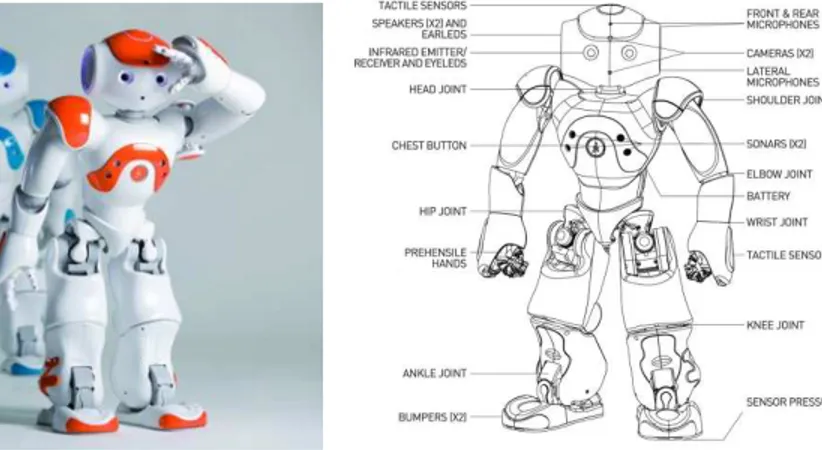
(a) The NAO NextGen robot (b) On board sensors and actuators

Figure 1: The humanoid platform NAO

All the following methods have been applied to the humanoid robot NAO. This robot is an af- 5

fordable and flexible platform. It has 25 degrees of freedom, and each motor has a Magnetic Rotary 6

Encoder (MRE) position sensor, which makes proprioception possible with a good precision (0.1◦per 7

MRE). Its sensing system include in particular two color cameras (see Figure 1). It is equipped with an 8

on-board Intel ATOM Z530 1.6GHz CPU, and programmable in C++ and Python. A stable walk API 9

is provided, but it is based only on the joint position sensors and the inertial unit (see Gouaillier et al. 10

(2010)). It is affected by the feet slipping: the robot orientation is often not precise. This API makes it 11

possible to control the robot position and speed. 12

Working on such a platform has undeniable advantages in terms of human-robot interaction, or 13

more generally with the environment, but it also has specific constraints. The reduced computational 14

power, limited field of view and resolution of the camera and unreliable odometry are very constraining 15

factors. The aim here is to get some localization information without adding any sensor and still being 16

able to run on line on the robot. 17

1.2

Related work

SLAM is a recurrent problem in robotics. It has been extensively covered, using metric, topological or 19

hybrid approaches. However, the existing algorithms often have strong prerequisites in terms of sensors 20

or computational power. Our goal here is to find a robust method on a highly constrained platform, 21

Metric SLAM is the most common type of SLAM. Most rely on a metric sensor, such as a laser

23

range sensor, a depth camera, a stereo pair, an array of sonars etc. Thrun (2002) presents a survey of

24

some algorithms in that category: Kalman filter based, such as FastSLAM by Montemerlo et al. (2002),

25

Expectation-Maximization (EM) algorithms by Thrun (2001), occupancy grids (originally from Elfes

26

(1989)), etc.

27

Vision based metric SLAM rely on landmarks position estimation to provide the map, using mostly

28

Kalman based approaches. For example Chekhlov et al. (2006) implement a SLAM based on

Un-29

scented Kalman Filter for position estimation and SIFT features for tracking: this method is designed

30

to deal with high levels of blur and camera movements. However, these algorithms require to have a

31

calibrated camera or a high resolution and frame rate, which is not available on the NAO: the extrinsic

32

parameters of the camera vary from one robot to another. A VGA resolution is usually enough for most

33

algorithms, but most existing algorithms use either a calibrated camera or a wider field of view than

34

what is available on NAO. A higher resolution is available, but at a limited frame rate and at the cost

35

of higher CPU usage. It is also worth noting that most hand-held visual SLAM implicitly rely on the

36

hypothesis that the tracked keypoints are high above the ground and so of good quality and relatively

37

easy to track. Among other related work, PTAM is very promising. The initial algorithm was described

38

in Klein and Murray (2007), improved and optimized for a smartphone in Klein and Murray (2008),

39

which is a setup quite close to NAO in terms of computing power and camera field of view, but does

40

not seem to be fully reliable yet.

41

The previous methods use sparse keypoint information. It is also possible to use dense visual

42

information to get qualitative localization. Matsumoto et al. (2000) implements navigation based on

43

omni-directional view sequences. This kind of approach is heavier in terms of computational power,

44

but more robust to blur, and less sensitive to texture quality. This is why it is also an interesting trail to

45

explore.

46

Several approaches already exist to provide the NAO robot with a navigation system, but they

47

all have strong prerequisites and / or require additional sensors. Some perform a metric localization

48

and estimate the 6D pose of the robot by adding some metric sensor: Hornung et al. (2010) use a

49

combination of laser range and inertial unit data, while Maier and Bennewitz (2012) use an Asus

50

Xtion Pro Live depth sensor set on the top of the head. Both require a pre-built 3D map of the static

51

environment, though Maier and Bennewitz (2012) also deals with dynamic obstacles. As far as vision

52

is concerned, Maier et al. (2011) use sparse laser data to detect obstacles and classify them using vision.

53

Osswald et al. (2010) estimate the pose using floor patches to perform reinforcement learning and reach

54

a destination as fast as possible. It is worth noting that adding any kind of sensor on the robot (a laser

head or 3D camera) affects the robot balance and walk. Chang et al. (2011) propose a method for the 56

fixed Robocup context, using only the regular sensors, but they rely on the specific field features. 57

The first aim of this article is to try out simple keypoints positions method, in order to be as light 58

as possible in terms of computational power, which means in particular avoiding Kalman based ap- 59

proaches. In section 2, we describe a lightweight keypoints position estimation and try to adapt it to 60

the NAO platform. We show that although we have good theoretical results, the application to the robot 61

is difficult. Despite this, in section 3, we use some of our observations to derive a partial localization 62

information, which consists in estimating the robot orientation, and test it both in simulation and on a 63

real robot. 64

2

A metric visual SLAM algorithm

2.1

A keypoint based metric SLAM

2.1.1 Notations and model 67

Let x be the planar position of the robot, and θr its orientation in the world reference. For each 68

keypoint indexed by i, we letpidenote its position in the world reference. The robot axes are described 69

in Figure 2. 70

Figure 2: Axes definition on the robot

Lettingω denote the angular velocity of the robot, u ∈ R the value of its velocity expressed in m/s, 71

(a) Notations in the world reference (b) Notations in the robot reference

Figure 3: Notations for the metric SLAM position estimation

axis X we end up with the following kinematic model for the motion of the robot:

73 dθr dt = ω dx dt = uRθX dpi dt = 0 (1) 74

This model is quite simple, but corresponds to the existing walk API, which provides a speed

75

control for translations and rotations. It is also possible to control the walk step by step, but since the

76

focus of this work is not on the walk control, we have kept the high level simple control approximation.

77

In the robot reference frame (X, Y, Z), the position of the keypoint i is the vector

zi(t) = R−θ(t)(pi− x(t))

The camera measurement being the direction (bearing) of the keypoint, for eachi the vector

yi(t) = 1 kzi(t)k zi(t) is assumed to be measured. 78

In the present paper, we propose a simplified two-step approach to the SLAM problem. First, the

79

odometry is assumed to yield the true values ofω and u, and a filter is built to estimate each keypoint’s

80

position, and then, using those estimates globally, the knowledge of ω and u is refined (that is, the

81

sensor’s biases can be identified). The present section focuses on the first step, that is, estimatingpi

82

from measurementyiand perfectly knownω, u.

Our approach is based on the introduction of the vectory⊥

i = Rπ/2yi. Letting′denote the transpo- 84

sition of a vector, and writing thaty⊥

i is orthogonal toyiwe have 85

0 = z′_i(t)y_i⊥(t)

= (R_−θ(pi− x(t)))′yi⊥(t)

= (pi− x(t))′(Rθ(t)y⊥i (t))

(2) 86

Introducing the vector ηi(t) = Rθ(t)y⊥i (t) that is yi⊥mapped into the world reference frame, we 87

thus have 88

(pi− x(t))′η(t) = 0 = η′(t)(pi− x(t)) (3) 89

The previous notations are illustrated on Figure 3: Figure 3a displays the notations in the absolute 90

world reference and Figure 3b in the robot reference. 91

(2) simplifies all following computations by performing a reference change. Contrary to what is 92

usually done, all observations are considered in the robot reference and not in an absolute reference. 93

Knowing at each time the previous relation (3) should be true,pi− x(t) and thus pi(up to an initial 94

translationx(0)) can be identified based on the observations over a time interval as the solution to a 95

linear regression problem (the transformed outputsη(t) being noisy). To tackle this problem on line, 96

three main possibilities can be thought of. 97

2.1.2 Gradient observer 98

The problem can be tackled through least squares, trying to minimize at each step the following cost 99

function: 100

C(t) = (η′

i(t)( ˆpi(t) − ˆx(t)))2 (4) 101

To do so, we propose the (nonlinear) gradient descent observer (5), the estimation ofx and θ being 102

a pure integration of the sensor’s outputs, and the estimation ofpi beingki > 0 times the gradient of 103

C(t) with respect to piat the current iteration: 104

dˆθ dt = ω dˆx dt = uRθ(t)ˆ e1 d ˆpi dt = −kiηi(t) ′_{( ˆp} i(t) − ˆxi(t))ηi(t) ∀i (5) 105

The gradient of the cost function with respect topiis: 106

Lete(t) denote the estimation error between the estimated keypoint position and the actual position

108

in the robot reference (7), i.e.

109

e(t) = R_θˆr(t)( ˆzi(t) − zi(t))

(7)

110

The following result allows to prove asymptotic convergence of the error to zero under some

addi-111 tional conditions. 112 Proposition 1. d dtke(t)k 2_{= −2k} i(η′i(t)e(t))2 ≤ 0 (8) 113

(8) proves that the estimation error is always non-increasing as the time derivative of its norm is

114

non positive. Moreover, if there existsT, ǫ, α > 0 such that

115

Z t+T t

ηiη′i

is a matrix whose eigenvalues are lower bounded by ǫ, and upper bounded by α, the estimation

116

error converges exponentially to zero (the input is said to be persistently exciting).

117 Proof. By construction: 118 d dtke(t)k 2 ₌ d dt(e(t) ′_e(t)) = 2e′de dt (9) 119

First we compute the error derivative:

120 de dt = d dt(Rθˆr(ˆz − z)) = d dt(Rθˆr(R−ˆθr(ˆp − ˆx) − R−θr(p − x))) = d dt((ˆp − ˆx) − Rθˆr−θr(p − x)) = dˆp dt − dˆx dt − d dt(Rθˆr−θr(p − x))) (10) 121 Now if we denote ˆθr(t) − θr(t) = ˜θ(t): 122 d dt(Rθ(t)˜ (pi− x(t)))) = d dt(˜θ(t)) d d˜θ(t)(Rθ(t)˜ (pi− x(t))) + R_θ(t)˜ dp dt − R_θ(t)˜ dx dt 123

We know that dˆ_dtθ = dθ_dt = ω by construction of the observer, sod˜θ(t)_dt = 0 and also thatdx_dt = uRθe1 124

anddp_dt = 0, as the observed point is considered fixed. 125

So 126 d dt(Rθ(t)˜ (p − x))) = −Rθ(t)˜ dx dt = −R_θ(t)˜ uRθe1 = −uR_θˆe1 127

So if we inject this in (10) we obtain 128

de dt = dˆp dt − uRθˆe1+ uRθˆe1 = dˆp dt 129 So 130 de dt = dˆp dt (11) 131

So, using (9) and (11): 132

d dtkek 2 _{= 2e}′dˆp dt = −2ke′η( ˆpi− ˆxi)η′ (12) 133 Now 134 ( ˆpi− ˆxi)η′ = (e + R_θ(t)˜ (p − x))η′ = eη′+ eR_θ(t)˜ (p − x)η′ 135

So if we use relation (3) we have 136

( ˆpi− ˆxi)η′ = eη′ 137

So finally if we inject this in (12) 138

d dtkek

2 _{= −2ke}′_ηeη′ _{= −2k(η}′_e)2 ₁₃₉

140

However in simulations, we see the convergence with such an observer can be very slow. This is 141

because the instantaneous costC(t) is only an approximation of the true cost function viewed as an 142

integral ofC(s) over all the past observations i.e. observed during the time interval [0, t]. For this 143

2.1.3 Kalman filtering

145

The solution of this problem could be computed using a Kalman filter approach. Since we do not have

146

any a priori knowledge of the keypoints positions, the initial covariance matrix would beP0 = ∞.

147

Although this approach is perfectly valid, we will take advantage of the simplicity of the current

148

problem and consider an even simpler solution, described in subsubsection 2.1.4. This way we avoid

149

having to take care of numerical issues due to the initial jump of the covariance matrix from an infinite

150

value to a finite one. We also avoid having to maintain a Riccati equation at each step.

151

Another similar solution would be to use a Recursive Least Squares (RLS) algorithm, with a

forget-152

ting factorλ < 1. The following simpler approach is closely related to RLS: it replaces the forgetting

153

factor by a fixed size sliding time window.

154

2.1.4 Newton algorithm over a moving window

155

Due to the simplicity of the problem, and having noticed equation (2), we choose the following

ap-156

proach over Kalman or RLS filtering.

157

A somewhat similar approach to RLS consists in using a Newton algorithm to find the minimum of

158

the cost functionC(s) integrated over a moving window. This has the merit to lead to simple equations

159

and to be easily understandable. The cost at its minimum provides an indication of the quality of the

160

keypoint estimationpˆi. We choose this simple alternative to Kalman filtering. Consider the averaged

161 cost 162 Q(t, p) = Z t t−T (ηiηi′(s)(p − x(s)))2ds (13) 163

It is quadratic inp. Its gradient with respect to p merely writes ∇Q(t, p) =

Z t t−T

ηiηi′(pi− x(s))ds = A(t)p − B(t)

The minimum is reached when the gradient is set equal to zero, that is

164

ˆ

p(t) = A−1(t)B(t) (14)

165

To be able to invert matrix A(t), it has to be of full rank. By construction, it is possible iff the

166

successive directions of the keypoint observations are not collinear. This means that the keypoint has

167

been observed from two different viewpoints, which is the case in practice when the robot moves and

168

the keypoint is not in the direction of the move.

169

The convergence speed of this algorithm depends on the size of the sliding window T . It also

170

depends on the determinant of matrixA(t), which is easily interpreted: the triangulation will be better

171

if we have observations which have very different bearings.

This algorithm can be interpreted as a kind of a triangulation. The cost function (13) can be inter- 173

preted as the sum of the distances from the estimated position to observation lines. 174

2.2

Adapting to the humanoid platform constraints

The previous algorithm is quite generic, but it requires that keypoints must be tracked robustly, and 176

observed under different directions over time. This means that a few adaptations must be made on the 177

NAO. 178

2.2.1 Images 179

(a) Side view (b) Top view

Figure 4: NAO robot head with camera fields of view

As shown in Figure 4, the on-board camera has a limited field of view. On the other side, the 180

keypoints observations must be as different from each other as possible, which is obtained at best when 181

the observed keypoints are observed in a perpendicular direction to the robot. 182

To compensate for this, we use the fact that the robot can move its head around and build semi- 183

panoramic images. The robot moves its head to five different positions successively, without moving 184

its base, stopping the head in order to avoid blur. Figure 5 shows an example of such a panorama. The 185

different images are positioned using the camera position measurement in the robot reference, which is 186

known with a precision under 1◦thanks to the joint position sensors. This means that it is not required 187

to run any image stitching algorithm, because this positioning is already satisfactory. 188

This makes it possible to have a larger field of view, and thus to track keypoints on the side of the 189

robot, which are the ones where the triangulation works at best. However, it requires the robot to stop 190

in order to have sharp and well positioned images. In practice, we have determined that the robot must 191

Figure 5: Example of panoramic image

The robot head is not stabilized during the walk, which means the head is moving constantly up

193

and down. Because of the exposure time of the camera, most of the images are blurred. There is also a

194

rolling shutter effect: since the top part of the image is taken before the bottom part, the head movement

195

causes a deformation of the image which seems “squeezed”. Because of these factors, it is necessary

196

to stop the robot to get usable images.

197

The observer described in subsubsection 2.1.4 has been implemented in C++ to run on board on

198

the robot.

199

2.2.2 Keypoints

200

The tracked keypoints are chosen for their computation cost and robustness. The keypoint detector is a

201

multi-scale FAST (Features from Accelerated Segment test, (Rosten and Drummond, 2006)) detector

202

because it is quick to compute and provides many points. The descriptor is Upright SURF or USURF,

203

which is a variation of SURF (Bay et al., 2006) which is not rotation invariant and lighter to compute

204

than regular SURF. The fact that the keypoints are not rotation invariant is an advantage here, because

205

it reduces the risk of confusion between points which are similar after a rotation, for example a table

206

border and a chair leg. This makes the tracking more robust and avoids false positives.

207

The keypoint tracking is performed by matching the keypoints descriptor using a nearest neighbor

208

search with a KdTree to speed up the search. A keypoint is considered matched when its second

209

nearest neighbor distance is sufficiently greater than the first nearest neighbor distance. This eliminates

210

possible ambiguities in keypoints appearance: such keypoints are considered not sure enough to be

211

retained.

212

The keypoint extraction and matching have been implemented in C++ using the OpenCV library

213

(see OpenCV). Both FAST and USURF have proved robust enough to blur, so that the tracking error

214

is usually less than a few pixels. The FAST detector has a pixel resolution, which means 0.09 degrees

215

for a VGA resolution.

(a) Stops 0 to 4 (b) Stops 5 to 8

Figure 6: Robot stopping positions during an exploration run

2.3

Results and limitations

The previous algorithm has been tested on several runs in office environment (see Figure 5). During 218

the runs, the robot walked around, stopping every 50cm to take a half panorama. The experiments were 219

recorded in order to be re-playable, and filmed in order to compare the estimated keypoint positions to 220

the real ones. 221

Figure 6 shows the different stopping positions of the robot during a run. The robot positions and 222

orientation are marked with red lines. Figure 5 was taken at the first stop of this run. 223

Figure 7 shows a successful keypoint position estimation. The successive robot positions are 224

marked with red arrows, where the arrow shows the direction of the robot body. The green lines 225

show the observed keypoint directions. The pink cross corresponds to the estimated keypoint position. 226

The runs have shown that there are many keypoint observations that cannot be efficiently used 227

for the observer. For each of these cases, a way to detect them and so ignore the keypoint has been 228

implemented. 229

Parallel keypoint observations can be problematic. If the keypoint observations are exactly parallel, 230

the matrix that has to be inverted is not of full rank. In practice, the observations are not exactly parallel, 231

so the matrix would be invertible in theory. This leads to estimations of keypoints extremely far away, 232

because of small measuring errors. To identify this case, we rely on the determinant of the matrix, 233

which must be high enough. Figure 8 shows an example of such observations: the observations are 234

nearly parallel, probably observing a keypoint very far away in the direction highlighted by the dashed 235

blue line. 236

Because of matching errors or odometry errors, the triangulation may be of low quality, resulting 237

Figure 7: Example of correct triangulation from keypoints observations

Figure 8: Parallel keypoints observations

the sum of distances from the estimated position to the observation to correlate its value with the size

239

of the zone where the keypoints could be. Figure 9 shows an example of low quality triangulations: the

240

estimated keypoint is 0.5m meters away from some observation lines. The triangulation zone is drawn

241

with striped lines. A threshold on the cost value has been set experimentally to remove this low quality

242

estimations.

Figure 9: Low quality triangulation

Sometimes inconsistent observations can still result in an apparently satisfactory triangulation. One 244

of the ways to detect this is to check that the estimated keypoint position is still consistent with the 245

robot field of view. Figure 10 shows that the intersection between observations 0 and 4 is inconsistent 246

because it is out of the robot field of view in position 4. This is the same for observations 0 and 8: the 247

intersection is behind both positions. The observation directions have been highlighted with dashed 248

blue lines, showing that the lines intersections should be invisible from at least one robot pose. To 249

avoid this case, the algorithm checks that the estimation is consistent with every robot position in terms 250

of field of view and distance (to be realistic, the distance must be between 20cm and 5m). 251

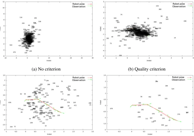
Figure 11 shows the influence of the different criteria on the keypoints estimation. The robot 252

trajectory is drawn in red, with the robot positions in green, and the keypoint identifiers are put at the 253

estimated positions. Note that the scale changes from one image to the other. Figure 11a presents the 254

results without any criterion: the keypoints are very dense, but some estimations are too far away to 255

be realistic. One keypoint is estimated 30m away for example, and most could not have been that far 256

because of the room configuration. Figure 11b adds the quality criterion: some points are eliminated, 257

and the distance values seem less absurd. The maximum distance is now around 6m. Figure 11c 258

reduces the number of keypoints by adding the consistency criterion: it is visible that the number of 259

unrealistic points has been reduced. For example, there are much less keypoints behind the first robot 260

position. Finally, Figure 11d also adds the matrix determinant criterion. The distance to the keypoints 261

Figure 10: Inconsistent keypoints observations: intersection behind the robot

However, even if the number of unreliable estimations has been greatly reduced, an examination of

263

the tracked keypoints has revealed that most of them are in fact false matches that happen to meet all

264

of the previous criteria. The ones that effectively were correct matches were correctly estimated, but it

265

was not possible to distinguish them from false matches.

266

This very high number of false matches comes from different causes. The first one is be perceptual

267

aliasing: in the tested environment, there were a lot of similar chairs that were often mixed up. Possible

268

solutions would be either a spatial check when matching keypoints and the use of color descriptors.

269

However this would not solve all problematic cases.

270

Another difficulty comes from the size of the platform. At the height of the robot, parallax effects

271

cause a large number of keypoints to appear or disappear from one position to the other. A way to solve

272

this would be to take more half panoramas, but this implies more stops, which is problematic because

273

the exploration is already very slow.

274

In fact, there were a lot of keypoints that were efficiently tracked. But they corresponded to

key-275

points that were very far away, or directly in front of the robot when it walked. These keypoints cannot

276

be used because they do not satisfy our estimation hypothesis. In section 3, we try to take advantage of

277

these points in another way.

278

In conclusion, even if simulation results seemed promising, and even if it was possible to meet

279

some of the requirements of the algorithm, it was not enough to track reliable, high quality keypoints

280

separately.

(a) No criterion (b) Quality criterion

(c) Quality and consistency criteria (d) Quality, consistency and determinant criteria

Figure 11: Effects of different criteria on the keypoint position estimations

3

A useful restriction: the visual compass

As explained in subsection 2.3, keypoints which are straight in front of the robot or which behave as if 283

they were infinitely far away can be tracked. These observations cannot be used to approximate their 284

positions, but they still can be useful. 285

3.1

From the metric SLAM to a compass

Keypoints that are infinitely far away (or behave as such) have a common characteristic: when the robot 287

orientation changes, they shift accordingly in the image. It is the same when the robot performs pure 288

rotation, without any hypothesis on the keypoint actual position. Ideally, when the orientation changes, 289

all keypoints will shift of the same number of pixels in the image. This shift depends on the image 290

resolution and camera field of view, and can be known in advance. Here we make the assumption that 291

rule to convert a pixel shift into an angular shift. This assumption is only a simplification, so a more

293

complex model could be used, and it is met in practice on the camera of NAO.

294

3.1.1 Observation of the deviation angle

295

Ideally, if all keypoints were tracked perfectly, and satisfying the desired hypothesis, only one pair of

296

tracked point would be required to get the robot orientation. However, this is not the case because

297

of possible keypoints mismatches, imprecisions in the keypoints position due to the image resolution.

298

The assumption that the robot makes only pure rotations is not true, because the head is going up and

299

down during the walk, and the robot torso is not exactly straight. This implies some pitch around the

300

Y axis and roll around the X axis which added to the yaw deviation around the Z axis (see Figure 2 for

301

the axes definitions). When the robot is going forward, because the tracked keypoints are not actually

302

infinitely far away, the zooming or dezooming effect will add to the shifting, and our assumptions will

303

be less and less valid.

304

To compensate for this effect, a possible solution is to rely on all tracked keypoints to get the most

305

appropriate global rotation. A way to this is to use RANdom SAmple Consensus (RANSAC) (or any

306

variation such as PROSac). A model with two pairs of matched keypoints is used to deduce the yaw,

307

pitch and roll angles.

308

To make the model computations easier, we will use the complex representation of the keypoints

309

position. Letz1 be the position of the first keypoint in the reference image, and z1′ its position in

310

the current image. z2 andz2′ are defined in a similar fashion for the second keypoint. We define the

311 following variables 312 θ = arg(z ′ 1− z2′ z1− z2 ) o = z′₁− z1eiθ (15) 313

The angles can then be obtained by the following equations, ifc is the image center coordinates:

314

ωx= θ

ωy = ℑ(o − (1 − eiθ)c)

ωz= ℜ(o − (1 − eiθ)c)

315

It is worth noticing that the model (15) is not usable for every couple of matched point. The

316

model assumes that this pair of points is consistent with the model. This is not the case for example if

317

the keypoints are mismatched. However this false computations will be eliminated by the RANSAC,

318

because they cannot have more inliers than a model based on valid points.

To compute the inliers for one particular model, we have to define a distance from one point to the 320

other. For a point pair(z, z′_{), we compute the theoretical image of z: 321}

˜

z = eiθz + o 322

The distance is then: 323

d = k˜z − z′k (16) 324

We can then use the model computations from (15) and the distance computation from (16) to 325

perform the algorithm. The number of inliers from the final best model can be used as an indication of 326

how reliable the computation is. In particular, this can be used when the assumption that keypoints are 327

infinitely far away becomes dubious, as in subsubsection 3.1.2. 328

The keypoints used are multi-scale FAST detector as before, but the chosen descriptor was the ORB 329

descriptor (Oriented BRIEF, see Rublee et al. (2011)) for speed and computational cost reasons. This 330

descriptor is a vector of 256 binary values, which are quicker to extract and to compare than the usual 331

SURF descriptors, with only on a slight difference in robustness. 332

In practice, the camera angular resolution is7 ∗ 10−3 _{radians per pixel for a 160x120 resolution 333}

(which is the one used here). This means that if we have an uncertainty of 5 pixels, which is a reason- 334

able upper bound for the uncertainty of the keypoint detection, this results in an uncertainty of about 2 335

degrees maximum, which is a considerable improvement from the uncorrected walk (see for example 336

Figure 16 for a comparison). 337

The robustness and precision of this method is linked to the keypoint density. In practice, most 338

indoors or outdoors environment have enough keypoints to provide a reliable heading estimation. 339

3.1.2 Control of the robot movement 340

The principle of our visual compass is to use this information to control the robot orientation. Letω 341

be the angle to rotate. Before rotating, the robot first turns its head towards a reference direction. This 342

direction is situated at the angle position−ω₂ in the initial robot reference, so that any rotation within 343

[−π, π] is possible. The robot then maintains its head in that direction and rotates its body towards 344

the final orientation. The head target position is0, and the base target position is ω₂, in the direction 345

reference. Letα be the head angle in the fixed reference and θ be the body angle.Their initial values 346

are0 and −ω₂ respectively. The robot is controlled with its body rotation speed ˙θ and with its head 347

Figure 12: PID controllers for the head and robot body

The control is done with two PID controllers, described in Figure 12. The observed variable is the

349

current angular deviation of the head in the fixed reference,α. We deduce the current deviation of theˆ

350

robot body using the internal position sensors of the robot, S. The desired robot body speed is then

351

computed. It is used to predict the head movement due the body movement∆αp= ˙θ∆t, which is then

352

added to the current observed angle for the error computation. This step has been added to make the

353

head tracking more robust for high rotation speeds.

354

For translations, it is possible to make the robot walk a straight line by simply adding a forward

355

speed ˙x. When the estimation starts being less reliable (see subsubsection 3.1.1), the robot stops going

356

forward, aligns itself in the desired direction and renews its reference image. This makes the reference

357

reliable again, and the robot can keep going forward.

358

3.2

Simulation results on Webots

359

To obtain quantitative results with a reliable ground truth measurement, we have used Webots simulator

360

from Cyberbotics. This simulator provides physics simulation along with various sensors simulation,

361

including cameras. A simulated world has been built to test the visual compass (see Figure 13) using

362

the simulator as a ground truth. This simulator emulates a real robot and reproduces the architecture

363

of the robot operating system, NAOqi. The simulator differs from the real world in the odometry

364

estimation which is slightly worse in the simulator (because the robot is slipping more) and the images

365

are more stable (because there is no motion blur or lighting conditions changes). However this is an

366

interesting validation step, and makes it possible to get repeatable and measurable experiments.

Figure 13: The simulated environment (using Webots)

Two different simulated experiments have been run. During each experiment, we record the esti- 368

mated angle from the compass, the ground truth position of the robot and the estimated position of the 369

robot by the odometry. The odometry and compass estimation are reset to the ground truth between 370

each new target movement. 371

Figure 14: Comparison of the robot angle estimations during pure rotations (two rotations of 20s each)

The first experiment makes the robot perform two consecutive pure rotations, of an angle π then 372

−π (each lasting around 20 seconds in the simulator). Figure 14 shows a comparison of the different 373

estimations of the robot base angle. The ground truth angle is drawn in dashed blue line, the compass 374

the odometry measurement drifts steadily during the movement, while the compass estimation stays

376

close to the ground truth.

377

Figure 15: Comparison of robot angle estimations during a translation (25s experiment)

The second experiment makes the robot walk in a straight line for about 25 seconds. Figure 15

378

shows a comparison of the estimations of the robot base angle (with the same display conventions as

379

the previous figure). This shows that the odometry has a nearly constant bias of approximatively 0.15

380

radians (around 9◦). This also shows that in the ground truth, the robot walks in a near straight line (or

381

at least, a set of parallel lines with a slight lateral shift). The estimated compass angle oscillates around

382

the ground truth, with a weak oscillation amplitude (0.05 radians).

383

Figure 16 compares the robot trajectory as estimated by the odometry and the ground truth

tra-384

jectory. The odometry trajectory is drawn as a full blue line, while the ground truth is represented

385

as a dashed green line. The oscillations come from the fact that the robot torso is oscillating during

386

the walk, and the oscillation period corresponds to the stepping period. Note that the odometry

un-387

derestimates the amplitude of these oscillations. The bias highlighted by Figure 15 can be seen quite

388

clearly, because the trajectory is clearly steadily drifting from the real trajectory, with a constant angle

389

of around 0.12 radians (about 7 degrees).

390

3.3

Results on the real robot

391

The compass has been integrated on the robot, with a C++ implementation based on the OpenCV

392

library. Figure 17 shows a typical output of the keypoint matching with the RANSAC model. The

Figure 16: Comparison of robot trajectories estimation during a translation (25s experiment)

Figure 17: Example of RANSAC output on keypoint matching

reference image is shown on top, and the current one on the bottom part. The inliers are marked in 394

green, while the outliers are drawn in red. This figure shows how all inliers behave consistently, here 395

with a global shift to the left. On the other hand, outliers correspond to inconsistent points, which are 396

due to false matches. Note that the rotation change between the two images is clearly visible in the 397

selected inliers. 398

Table 1 shows the CPU usage of the algorithm on the robot for available resolutions of the camera. 399

For the walk corrections, the typical parameters is 160x120 and 15fps. The maximum resolution is 400

only available at 5 frames per second, so around 36% CPU. Note that the results are significantly better 401

Resolution 160x120 320x240 640x480 1080x960

5 fps 2% 4% 10% 36%

15 fps 6% 11% 31% NA

30 fps 13% 23% 60% NA

Table 1: Comparison of CPU usage for different resolution and frame rates

Figure 18: Evolution of head and base speeds with time (9s experiment)

PID parameters have been tuned for the robot. The following results are presented for a desired

403

rotation of π₂, which lasted around 10 seconds. Figure 18 presents the computed speeds in the robot

404

reference. Both speeds are capped for walk stability. The head speed (blue full line) is drawn is

405

compensating both the base speed and the errors on the head and the base position. The base speed (in

406

green dashed line) is first capped then decreases slowly. When the body angle reaches the destination,

407

the robot is stopped immediately, which explains why the speed is not necessarily zero at the end of

408

the experiments.

409

Figure 19 shows the evolution of the head angle in the fixed reference. The head angle (in blue full

410

line) is oscillating around the consign (in green dashed line).

411

Figure 20 shows the evolution of the base angle in the fixed reference. The goal value is π₄ and the

412

start value is−π₄. The robot stops when the error is under a fixed threshold. Overshoot is compensated

413

by taking one last measurement at the end of the rotation to retrieve the final angle, which makes it

414

possible to correct this overshoot later on, if necessary.

Figure 19: Evolution of head angle with time (9s experiment)

Figure 20: Evolution of base angle with time (9s experiment)

Future plans include to use a motion-capture device to get quantitative and precise data on a real 416

NAO robot, in order to confirm the simulation experiments. 417

4

Conclusion

In this article, we have presented our work on localization and mapping on a constrained humanoid 419

keypoints positions. We have added a series of adaptations for our platform, including increasing

421

the field of view by moving the head and compensating false matches by checking some consistency

422

conditions and estimation quality. However, the final results have not proven satisfying enough on

423

NAO. This comes in particular from the small robot height, which makes it very difficult to extract

424

high quality keypoints and track them. The robot limited field of view is also an issue, along with its

425

reduced speed, which makes frequent stops long and tedious. It might be possible to reuse some of this

426

work on taller robots, such as ROMEO for example, or some other platform, because there are very

427

few requirements except the ability to track keypoints.

428

Nevertheless, from our work on keypoint tracking, we have been able to derive a partial

localiza-429

tion information, the robot orientation. To do so, we have built an efficient visual compass which is

430

based on matching reference image keypoints with the current observed keypoints, and deducing the

431

current robot rotation. FAST keypoints with ORB descriptors are extracted, and their global rotation is

432

computed using a RANSAC scheme. PID controllers make it possible to control the robot orientation

433

precisely, performing rotations and walking along straight lines with much higher precision that the

434

open loop odometry. The implementation is running in real time on the robot, and its accuracy has

435

been controlled quantitatively on simulator and qualitatively on a robot. Future work includes getting

436

quantitative data on a real robot with motion capture.

437

In future work we will look more closely at other type of vision based approaches, such as dense

438

visual method base on image correlation, whose characteristics and weaknesses are complementary to

439

the sparse algorithms described in this article.

440

References

441

H. Bay, T. Tuytelaars, and L. Van Gool. Surf: Speeded up robust features. Computer Vision–ECCV

442

2006, page 404–417, 2006.

443

Chun-Hua Chang, Shao-Chen Wang, and Chieh-Chih Wang. Vision-based cooperative simultaneous

444

localization and tracking. In 2011 IEEE International Conference on Robotics and Automation

445

(ICRA), pages 5191 –5197, May 2011. doi: 10.1109/ICRA.2011.5980505.

446

Denis Chekhlov, Mark Pupilli, Walterio Mayol-Cuevas, and Andrew Calway. Real-time and robust

447

monocular SLAM using predictive multi-resolution descriptors. In Advances in visual computing,

448

page 276–285. Springer, 2006. URL http://link.springer.com/chapter/10.1007/

449

11919629_29.

Cyberbotics. Webots simulator. URL http://www.cyberbotics.com/overview. 451

A. Elfes. Using occupancy grids for mobile robot perception and navigation. Computer, 22(6):46–57, 452

1989. 453

D. Gouaillier, C. Collette, and C. Kilner. Omni-directional closed-loop walk for NAO. In 2010 10th 454

IEEE-RAS International Conference on Humanoid Robots (Humanoids), pages 448 –454, December 455

2010. doi: 10.1109/ICHR.2010.5686291. 456

A. Hornung, K.M. Wurm, and M. Bennewitz. Humanoid robot localization in complex indoor envi- 457

ronments. In 2010 IEEE/RSJ International Conference on Intelligent Robots and Systems (IROS), 458

pages 1690 –1695, October 2010. doi: 10.1109/IROS.2010.5649751. 459

Georg Klein and David Murray. Parallel tracking and mapping for small AR workspaces. In Proc. 460

Sixth IEEE and ACM International Symposium on Mixed and Augmented Reality (ISMAR’07), Nara, 461

Japan, November 2007. 462

Georg Klein and David Murray. Compositing for small cameras. In Proc. Seventh IEEE and ACM 463

International Symposium on Mixed and Augmented Reality (ISMAR’08), Cambridge, September 464

2008. 465

D. Maier and M. Bennewitz. Real-time navigation in 3D environments based on depth camera data. 466

In Proceedings of the IEEE-RAS International Conference on Humanoid Robots (HUMANOIDS), 467

2012. 468

D. Maier, M. Bennewitz, and C. Stachniss. Self-supervised obstacle detection for humanoid navigation 469

using monocular vision and sparse laser data. In 2011 IEEE International Conference on Robotics 470

and Automation (ICRA), pages 1263 –1269, May 2011. doi: 10.1109/ICRA.2011.5979661. 471

Y. Matsumoto, K. Sakai, M. Inaba, and H. Inoue. View-based approach to robot navigation. In 2000 472

IEEE/RSJ International Conference on Intelligent Robots and Systems, 2000. (IROS 2000). Pro- 473

ceedings, volume 3, pages 1702–1708 vol.3, 2000. doi: 10.1109/IROS.2000.895217. 474

M. Montemerlo, S. Thrun, D. Koller, and B. Wegbreit. FastSLAM: a factored solution to the simul- 475

taneous localization and mapping problem. In Proceedings of the National conference on Artificial 476

Intelligence, page 593–598, 2002. 477

S. Osswald, A. Hornung, and M. Bennewitz. Learning reliable and efficient navigation with a

hu-479

manoid. In 2010 IEEE International Conference on Robotics and Automation (ICRA), pages 2375–

480

2380, 2010. doi: 10.1109/ROBOT.2010.5509420.

481

Edward Rosten and Tom Drummond. Machine learning for high-speed corner detection. Computer

482

Vision–ECCV 2006, page 430–443, 2006.

483

Ethan Rublee, Vincent Rabaud, Kurt Konolige, and Gary Bradski. ORB: an efficient alternative to SIFT

484

or SURF. In Computer Vision (ICCV), 2011 IEEE International Conference on, page 2564–2571,

485

2011.

486

Sebastian Thrun. A probabilistic on-line mapping algorithm for teams of mobile robots. The

In-487

ternational Journal of Robotics Research, 20(5):335–363, January 2001. ISSN 0278-3649,

1741-488

3176. doi: 10.1177/02783640122067435. URL http://ijr.sagepub.com/content/20/

489

5/335.

490

Sebastian Thrun. Robotic mapping: A survey. In Exploring Artificial Intelligence in the New

Mille-491

nium. Morgan Kaufmann, 2002.

492

E. Wirbel, B. Steux, S. Bonnabel, and A. de La Fortelle. Humanoid robot navigation: From a visual

493

SLAM to a visual compass. In 2013 10th IEEE International Conference on Networking, Sensing

494

and Control (ICNSC), pages 678–683, 2013. doi: 10.1109/ICNSC.2013.6548820.