HAL Id: hal-01998837
https://hal.archives-ouvertes.fr/hal-01998837v2
Submitted on 16 Dec 2020
HAL is a multi-disciplinary open access archive for the deposit and dissemination of sci-entific research documents, whether they are pub-lished or not. The documents may come from
L’archive ouverte pluridisciplinaire HAL, est destinée au dépôt et à la diffusion de documents scientifiques de niveau recherche, publiés ou non, émanant des établissements d’enseignement et de
Multi-temporal assessment of power system flexibility
requirement
Thomas Heggarty, Jean-Yves Bourmaud, Robin Girard, Georges Kariniotakis
To cite this version:
Thomas Heggarty, Jean-Yves Bourmaud, Robin Girard, Georges Kariniotakis. Multi-temporal as-sessment of power system flexibility requirement. Applied Energy, Elsevier, 2019, 238, pp.1327-1336. �10.1016/j.apenergy.2019.01.198�. �hal-01998837v2�
Multi-temporal assessment of power system flexibility
requirement
Thomas Heggartya,b, Jean-Yves Bourmauda, Robin Girardb, Georges Kariniotakisb
aRéseau de Transport d’Electricité, La Défense, FrancebMINES ParisTech, PSL
University, Center for processes, renewable energies and energy systems (PERSEE), Sophia-Antipolis, France.
Abstract
In power systems, flexibility can be defined as the ability to adapt to variabil-ity and uncertainty in demand and generation. Various ongoing changes in the power system are impacting the need for flexibility. We propose a novel methodology to (i) evaluate annual, weekly and daily flexibility requirements through a set of frequency spectrum analysis based metrics, (ii) examine the sensitivity of these flexibility requirements to five variables: the degree of network interconnection and the penetration of wind power, solar power, electric heating and cooling. The proposed methodology is validated on a case study focusing on the French power system, while accounting for its elec-trically connected neighbours. We provide an estimation of how flexibility requirements are likely to evolve in years to come; the use of global sensi-tivity analysis allows the identification of the variables responsible for these evolutions. The presented methodology and results can be used to identify future challenges, to evaluate the market potential of flexibility solutions and to assess the implications of policy decisions.
Keywords: Power system flexibility, renewable energy sources impacts, load temperature sensitivity, frequency spectrum analysis, global sensitivity analysis
Nomenclature Input parameters
c, cc country, central country
Lcool(t) electric cooling load time series (MW) Lheat(t) electric heating load time series (MW)
Lti(t) temperature insensitive load time series (MW) S(t) solar generation time series (MW)
W (t) wind generation time series (MW) Proposed metrics
F ER(T ) Flexible Energy Requirement, for a given timescale (annual, weekly or daily)
F P R(T ) Flexible Power Requirement, for a given timescale (annual, weekly or daily)
Long-term variables impacting flexibility requirement I interconnection capacity (MW) pcool electric cooling penetration (unitless) pheat electric heating penetration (unitless) psolar solar penetration (unitless)
pwind wind penetration (unitless) 1. Introduction
1.1. Context
Flexibility has always been required in power systems in order to match supply and demand1. Driven by the need to meet green house gas emissions reduction targets, the gradual move from flexible conventional generation to Variable Renewable Energy Sources (VRES) induces growing variability and uncertainty, making the supply and demand matching exercise increas-ingly challenging [1]. A significant number of levers may be activated to provide flexibility to a power system which may be regrouped in four main categories: flexible generation, flexible demand, energy storage and network interconnection [2]. The wide variety of their characteristics and constraints makes their simultaneous modelling complex, calling for literature to take
1In this paper, only flexibility for adequacy purposes is considered. In Europe,
supply-demand matching is performed at the national scale, hence in this study, the power system can be understood as the national grid.
a step back from the lever view and try to understand, define and quantify flexibility [1, 2, 3, 4, 5, 6]. Several definitions have been presented, all are in general agreement; flexibility is understood as the power system’s ability to cope with variability and uncertainty in demand and generation.
Variability and uncertainty in demand and generation occur on several timescales. On the long-term (more than a year), matching supply and de-mand is made uncertain by the difficulty to predict VRES development, the evolution of consumer habits, economic growth etc. On the medium term (annual, weekly and daily horizons), power system operators must face cycli-cal variations in net load (load minus VRES generation). On the short-term (intra-day), power system operation is constrained by uncertainty through incidents and forecastability of demand and VRES generation.
This paper proposes (i) a set of metrics quantifying annual, weekly and daily flexibility requirements (i.e. the amount of flexibility resource needed for each timescale, not presuming the lever that might supply it), and (ii) a methodology to analyse the sensitivity of these requirements to five un-certain long-term variables: the degree of network interconnection and the penetration of wind power, solar power, electric heating and cooling.
1.2. Review of flexibility metrics
Researchers have proposed a variety of flexibility metrics illustrating dis-tinct properties or phenomena, leading authors to suggest that flexibility cannot be understood through a single indicator [1, 2, 7]. Depending on their role, metrics can be split into three categories [7]: those who evaluate a resource’s ability to provide flexibility, a system’s ability to provide flexi-bility and a system’s need for flexiflexi-bility. Table 1 provides a non-exhaustive overview of metrics used to provide insight for long-term planning.
Other studies aiming to evaluate a system’s need for flexibility use storage as a proxy for flexibility, i.e. they try to determine how much storage would be needed to cope with variability and uncertainty. Requirement is therefore expressed in terms of power and energy. Such studies have focussed on short-term phenomena, such as the mismatch between scheduled generation and actual load [8] or reducing the difference between forecast and actual wind power generation [9]. Longer timescale phenomena can also be observed with these metrics [10, 11]. However, in these last two studies, power and energy metrics do not express a flexibility requirement inherent to a load curve, but provide storage characteristics, which were jointly optimised with generation, VRES curtailment or network (which are themselves flexibility providers).
Table 1: Non-exhaustive overview of flexibility metrics for long-term planning purposes
Type Role Metric Comment
Evaluating a resource’s
ability to provide flexibility
Compare different flexibility resources, commonly used as
input parameters in dispatch models
Ramp rate
Characterise flexible generation, flexible load
or storage [12] Minimum up/down time
Start-up time Response time Minimum power output
Energy capacity Characterises storage or flexible load [13] Rebound effect Characterise flexible load [13] Recovery period Evaluating a system’s ability to provide flexibility
Analyse long-term power system data or the outputs of dispatch models, allowing a straightforward comparison
of complex systems
Weighted sums of resource
flexibility metrics without a dispatch model [14]Analysis can be performed Loss Of Load Probability Standard adequacy metrics
giving probability, duration and volume of loss of load [15] Loss Of Load Duration
Expected Unserved Energy
Periods of Flexibility Deficit there is less flexible resourceNumber of periods where available than required [3, 16] Insufficient Ramping
Resource Expectation Probabilistic equivalent to the Periodsof Flexibility Deficit metric [3, 16] Expected Unserved Ramping Reflects the magnitude ofthe ramping shortage [16]
Evaluating a system’s need
for flexibility
Analyse net load curves to evaluate implications of energy
policy decisions and improve the understanding
One or multiple hour ramp Derivative of net load overtime, expressed in MW or as a percentage [4, 5, 17] Ramp acceleration net load over time [5]Double derivative of
The literature already provides ample metrics evaluating a system’s need for intra-day flexibility. However, flexibility is a multi-timescale issue [17]. This paper builds upon and generalises state-of-the-art approaches to express flexibility requirement on the annual, weekly and daily timescales. Flexibility requirement, inherent to a load curve, is expressed in terms of power and energy.
1.3. Variables impacting flexibility requirement
Power system flexibility requirement is affected by several uncertain long-term variables; VRES penetration has been the most investigated. An early study by Holttinen et al. [17] analysed the effect of large wind penetrations on ramps, showing an increase in their magnitude and change in their oc-currence patterns, both diurnal and monthly. Using one and multiple hour ramps, Huber et al. [4] have extended the analysis to both onshore wind and solar photovoltaics impacts on European net load curves. Deetjen et al. [5] have performed a similar study on the ERCOT system, with a wide vari-ety of ramp derived indicators. Both of these studies highlight the fact that increased solar photovoltaics penetration generates a significant additional ramping requirement, the effect of wind is much more limited. In another study, Belderbos et al. [10] optimise a storage portfolio for different so called remaining load profiles, where both VRES and conventional generation are subtracted from load. Steinke et al. [11] aim to determine the backup gen-eration required in a high VRES share system, examining the potential role of storage and interconnection. In both these last two studies, it can be seen that for increased VRES shares, the storage energy capacity requirement is much more affected than the power capacity requirement.
The specificity of network interconnection when compared to other flex-ibility solutions makes it quite complicated to characterise it in the same way. As such, the degree of interconnection can be an interesting parameter to vary when evaluating flexibility requirement. Expressing the ability of grid interconnection to average net load over space has been a focus point of several aforementioned studies [4, 11]. The European project e-Highway 2050 [18] developed a scenario based methodology to determine least regret options for European grid expansion. In two other studies, Fursch et al. [19] and Kristiansen et al. [20] highlight the grid’s role in capacity expansion modelling.
Another key variable affecting flexibility requirement is load temperature sensitivity, which so far has not been treated as such by the literature. Papers
on the subject adopt a policy approach, examples of which are analyses of long-term climate change impacts on European load curves [21, 22], or the implications of an ongoing increase of temperature sensitivity of summer electricity demand on asset maintenance scheduling [23]. Several papers issue a warning to countries considering heat electrification, in a move towards heat decarbonisation [24, 25, 26]. The security of supply risk and the approximate associated cost resulting from this added load variability is quantified. 1.4. Key contributions and paper structure
Flexibility reflects the power system’s ability to adapt to variability and uncertainty in demand and generation, which occur on different timescales. The research presented in this paper aims to determine (i) how and (ii) why medium-term (annual, weekly and daily) flexibility requirement will evolve under the influence of long-term (more than a year) variables. These are the first two steps towards determining how the system is to adapt to its changing environment.
Studies evaluating the need for flexibility have so far been short-term (intra-day) focussed. On the medium-term, to the best of our knowledge, there has been very little work on quantifying flexibility requirement. This paper bridges this gap by proposing a set of frequency spectrum analysis based indicators that allow the separation of annual, weekly and daily flexi-bility requirements, the three relevant timescales when considering load and net load (load minus VRES generation) variability.
Flexibility requirement is affected by several uncertain long-term vari-ables, which have up to now been investigated separately. This paper pro-vides novel insights by simultaneously examining flexibility requirement sen-sitivity to the penetration of wind power, solar power, electric heating and cooling, as well as to the degree of interconnection. The impact of these variables on each timescale is examined, along with the interactions between variables. An estimation of how flexibility requirements are expected to evolve is provided; the use of Global Sensitivity Analysis (GSA) enables the identification of the variables responsible for the expected evolutions.
Another strength of this study lies with the input data used, which gives a thorough probabilistic view: the load and VRES time series used are based on 200 years of Météo-France synthetic weather data, expressing temporal, spatial and inter-variable correlations.
This paper starts by presenting the proposed methodology (section 2), then applies it to a case study (section 3) focusing on the French power
system, while accounting for its electrically connected neighbours. Chosen for data availability reasons and authors’ personal interests, it is an inter-esting system to examine as all five of the considered long-term variables are expected to evolve significantly in years to come, as France undergoes its energy transition. Results for other European countries are occasionally shown or mentioned to provide a reference and discuss limitations in results. Sections 2 and 3 are given an introduction to specify their purpose and inter-nal structure. The conclusion (section 4) summarises key findings, discusses differences in results had the case study been performed on another country and briefly mentions ongoing work.
2. Methodology 2.1. Introduction
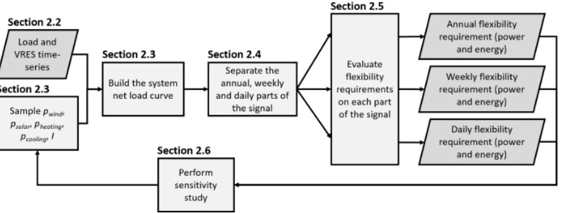
A general overview of the proposed methodology is shown in figure 1, it also states in which subsection each step is detailed.
Figure 1: General overview of the proposed methodology
2.2. Data used
Météo-France, the French national meteorological service, has developed the ARPEGE-Climat model which, coupled with ocean, sea ice and surface models, simulates long-term climate evolution [27]. With energy related ap-plications in mind, Météo-France has used this model to produce 200 years of synthetic weather time series, representative of our current climate [28].
Covering the whole globe, outputs are expressed at hourly and, for Europe, 0.5° latitude and longitude resolutions.
RTE, the French Transmission System Operator (TSO), has derived wind and solar generation as well as load data from these weather time series, al-lowing temporal, spatial and inter-variable correlations to be kept [29]. Used in numerous studies including the French adequacy report, legal obligation of RTE [30], these time series are the basis of the analysis presented in this paper, defined at hourly and national resolutions, for France and all its elec-trically connected neighbours. Load is modelled using a bottom-up approach [30]; electric heating and cooling load could therefore be varied independently from temperature insensitive load.
2.3. Building the system net load curve
As shown in equation 1, each country’s load is composed of three parts: a temperature insensitive one, a heating one and a cooling one.
Lc(t) = Lcti(t) + pcheatLcheat(t) + pccoolLccool(t) (1) where: t time, from hour 1 to hour 8760 * 200
c country
pheat electric heating penetration (unitless) pcool electric cooling penetration (unitless)
Lti(t) temperature insensitive load time series (MW) Lheat(t) electric heating load time series (MW)
Lcool(t) electric cooling load time series (MW) Each country’s net load is defined as follows:
Lcnet(t) = Lc(t) − pcwind L c WcW c(t) − pc solar Lc ScS c(t) (2) where: pwind wind penetration (unitless)
psolar solar penetration (unitless)
W (t) wind generation time series (MW) S(t) solar generation time series (MW)
Lc, Wc, Sc 200 year mean load, wind and solar generation The system net load curve can then be built, on the basis of which flex-ibility requirements can be evaluated. This curve, defined in equation 3, is
composed of a central country’s net load and parts of its neighbours’ net loads.
Lsystemnet (t) = Lccnet(t) +X c
Ic LcL
c
net(t) (3)
where: cc central country
I interconnection capacity (MW)
For the purpose of Global sensitivity analysis, several tens of thousands of combinations of I, pwind, psolar, pheat and pcool are sampled from uniform distributions within specific intervals.
Ic represents the capacity of country c’s link with the central country. Divided by c’s mean load, it indicates the proportion of c’s net load that is included in the system net load. For each neighbouring country, a specific in-terval is defined based on current and prospective interconnection capacities. A single relative position inside those intervals is sampled. For example, if countries A and B have intervals of [2000,4000] and [0,1000], a result of the sampling could be IA = 2800MW and IB = 400 MW.
pwind represents the share of load covered by wind generation, averaged over the 200 years of synthetic data. Multiplied by the 200 year mean load over the 200 year mean wind generation, it acts as a scaling factor of a homothetic transformation, ensuring that the wind generation time series covers the required load share. psolar works in a similar way. The sampling of pwind and psolar is done in the same way as I: each country is given an interval reflecting local potential and objectives and a single relative position in those intervals is sampled. In other words, VRES deployment is assumed to be synchronous across countries, but each at its own pace.
pheat and pcool are factors that reflect the volume of electric heating and cooling load respective to an initial situation. Individual country policy re-garding heating cannot be assumed to be synchronous (e.g. France is trying to reduce its electric heating demand while the UK and Germany are consid-ering heat electrification). Therefore, only the central country’s pheatand pcool were varied. A country’s flexibility requirement sensitivity to it’s neighbours’ load temperature sensitivity could also be evaluated, but this would require adding variables to be sampled, severely affecting computational time. 2.4. Separating the signal components
Load curves show clear cyclical patterns of various time periods: de-mand is higher during the day than during the night, higher during weekdays
than the weekend, and either higher in summer or winter depending on ge-ographical location. These patterns are sufficiently deterministic that, using a Fourier series based model, Yukseltan et al. [31] were able to predict Turk-ish national load within 3% Mean Absolute Percentage Error. Frequency based approaches have also been adopted for storage sizing [8, 9, 10, 32], for short-term VRES forecasting [33, 34, 35] or simply as a visualisation tool to complement the time domain vision [36, 37].
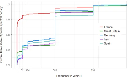
Figure 2 offers a view of national load curves in the frequency domain, expressed as a cumulative share of power spectral density. The load data used is the one described in section 2.2, with 2017 electric heating and cool-ing penetrations. It can be seen that a selected few frequency components (annual, weekly and its harmonics, daily and semi-daily) contain most of the information carried in the signal. It can also be seen that the balance between these frequency components varies from one country to another, the most obvious example being the very significant annual component in the French load curve due to the high penetration of electric heating.
Figure 2: Cumulative frequency spectrum share of national load curves
Flexibility requirements were to be quantified for three timescales: an-nual, weekly and daily. Hence, net load curve data was first fed through a Discrete Fourier Transform (see equation 4), then, using a similar method to
the one used by Makarov et al. [8], band pass filters with unit magnitude within the band and zero magnitude outside the band were applied, with cut off frequencies at 20 and 180 year-1 i.e. periods of about 18 and 2 days. The DC offset was removed prior to the filtering process.
Xf = N −1 X t=0
xte−i2πf t/N f = 0, ..., N − 1 (4) The three resulting signals were then passed back into time domain using the inverse Fourier Transform.
2.5. Evaluating flexibility requirement
For each year of the low-frequency time series, the difference between its minimum and maximum levels was recorded; the resulting vector of 200 values was defined as the annual flexible power requirement (F P R(a)). Sim-ilarly, the integral of the low frequency time series was computed, obtaining what could be equated as a "stock level". The difference between the mini-mum and maximini-mum of this "stock level" was recorded; the resulting vector of 200 values was defined as the annual flexible energy requirement (F ER(a)). The process was repeated for each week of the mid-frequency and each day of the high-frequency parts of the load curve signal, obtaining 200*52 and 200*365 values for weekly and daily requirements respectively, both in terms of power and energy (F P R(w), F ER(w), F P R(d), F ER(d)).
In order to reflect the benefit brought by interconnection, the resulting flexibility requirements were then normalised by the system’s maximum load for the flexible power requirement and by the system’s mean annual demand for the flexible energy requirement (n.b. not net load).
2.6. Global sensitivity analysis
Flexibility requirement sensitivity to X = [I, pwind, psolar, pheat, psolar]was evaluated using the global sensitivity analysis Sobol method [38]. This variance-based method quantifies the contribution of each input variable to the output’s variance. It has been used regularly on energy related matters [39, 40, 41, 42, 43] and shows significant advantages over other sensitivity analysis methods: it makes no assumption on the model’s behaviour (e.g. linearity), provides straightforward interpretation through quantitative rank-ing of variable importance and is capable of evaluatrank-ing interactions effects between variables [44]. However, the method assumes variable independence
and can be computationally expensive, all the more so as the number of considered variables increases [44, 45].
Based on Monte Carlo runs of the flexibility requirement module previ-ously described, the method calculates first order (see equation 5) and total (see equation 6) Sobol indices.
Si = VXi(EX∼i(Y | Xi))
V (Y ) (5)
STi =
EX∼i(VXi(Y | X∼i))
V (Y ) (6)
The numerators in equations 5 and 6 respectively represent "the expected reduction in variance that would be obtained if Xi could be fixed" and "the expected variance that would be left if all factors but Xi could be fixed" [45]. Si therefore gives the effect of factor by itself, while STi gives the total effect
of a factor, including its interactions with other factors.
The Sobol method needs a single output value to work with, not a vector. As a result, the sensitivity analysis was performed on the 95th percentile of flexibility requirement distributions. This is a fairly arbitrary choice, how-ever, varying the chosen percentile between 90 and 100 was shown to have negligible impact on results.
3. Case study 3.1. Introduction
GSA has certain limits which prevent it from providing a full picture of the flexibility problem. If it expresses flexibility requirement’s sensitiv-ity to input variables, it does not give the flexibilsensitiv-ity requirement itself nor its balance between different timescales, it does not convey the sign of the output’s sensitivity to an input variable (positive or negative contribution to flexibility) and it ignores effects outside of the chosen intervals.
For these reasons, the case study will start by setting the context by applying the flexibility requirement sizing method to current load curves. The impact of the input variables on flexibility requirement will then be illustrated by a few 2 dimensional cuts of the 5 dimensional problem, for a wide range of values. Finally, a prospective power system’s flexibility requirements will be presented, GSA will be used to express each input variable’s contribution to flexibility requirement evolution.
3.2. Base case
The method described in section 2.5 was applied to the data described in section 2.2. Load curves were constructed using 2017 electric heating and cooling levels, each country was treated by itself i.e. no interconnections were taken into account, VRES generation curves were not deducted from the load.
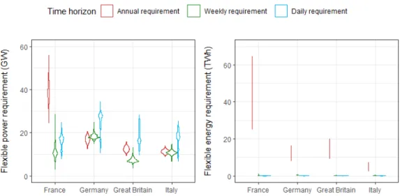
The results of the flexibility requirement evaluation are shown using two violin plots in figure 3. This graphical representation shows the full distribu-tion of flexibility requirements (200, 200*52 and 200*365 values for annual, weekly and daily requirements respectively). The width of each distribution has been normalised so that the area of each violin in a plot is equal. A summary of the considered power systems’ modelled demands is shown in table 2.
Table 2: Summary of considered power systems’ demand
France Germany Great Britain Italy Mean annual
load (TWh) 480 553 329 309 Peak load (GW) 112.2 86.9 63.7 54.4
The flexible power requirement is of the same order of magnitude for the three considered time horizons. Conversely, the flexible energy requirement is much higher for longer timescales: the annual requirement is 100 to 1000 times more important than the daily requirement. This general observation was also made in previous papers [8, 9, 10].
It can also be noted that for the flexible power requirement, the bal-ance between the three time horizons is not the same in each country. In France, the electric heating penetration induces a very high annual flexibility requirement, relative to the country’s annual and peak load. This sensitivity to temperature also generates particularly wide distributions of annual and weekly requirements, both in terms of power and energy.
3.3. Input variable impact on flexibility requirement
Network interconnection, wind, solar, electric heating and cooling pene-trations all affect flexibility requirement in different ways, on different time-scales and to various degrees. Bearing succinctness and clarity in mind, a select number of level-plots of flexibility requirement with respect to pairs
Figure 3: Flexibility requirements for different timescales and different countries. Electric heating and cooling levels are at 2017 levels, VRES generation has not been deduced from the load, interconnection has not been taken into account.
of input variables are presented. The effect of varying other variables is discussed when relevant.
3.3.1. Annual flexibility requirement
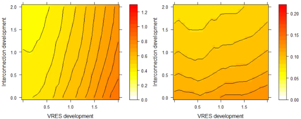
Figure 4 shows the 95thpercentile of the need for annual flexible power and energy observed in the French net load curve (F P R(a) and F ER(a)). Again, the choice of the 95th percentile is fairly arbitrary, but varying the percentile between 90 and 100 had negligeable impact on the general shape of results. The requirements are expressed in terms of solar and wind penetrations (0.3 wind indicates that on average, 30% of annual energy demand is covered by wind generation). Electric heating and cooling were set to their 2017 value, interconnection was set to zero. As mentioned in section 2.5, the power requirement was normalised by the system’s maximum load (n.b. not net load). Similarly, the energy requirement was normalised by the system’s mean annual demand. For reference, in 2017, France had solar and wind penetrations of about 2% and 5% respectively.
From a yearly perspective, solar generation and French electricity demand are out of phase, hence solar penetration increases the annual flexibility re-quirement. For wind generation, the situation is more complex: it is in
Figure 4: 95th percentile of annual flexible power requirement F P R(a) in MW/MW
(normalised by system maximum load, left) and energy requirement F ER(a) in TWh/TWh(normalised by system mean annual demand, right) in terms of wind and solar penetrations
phase with net demand up to a certain threshold under which wind pen-etration reduces the flexibility requirement. This threshold is high for the flexible energy requirement, however, due to its volatility, wind power quickly becomes detrimental where flexible power requirement is concerned.
From the direction of isolines, it can be seen that when a VRES type dominates, the flexible power requirement is determined solely by that type’s penetration. This is not the case for the flexible energy requirement which mostly depends on solar penetration.
Maximising VRES penetration for a given annual flexibility requirement will give a wind dominated electricity mix (more so for energy than power). This conclusion is affected if electric heating penetration is reduced: this causes a reduction in flexibility requirement, particularly in solar dominated mixes. For the energy requirement, it also reduces the threshold beyond which wind becomes detrimental (this threshold is beyond 50% wind pene-tration for the 2017 French situation). Another illuspene-tration of this can be seen by analysing the situation of different countries: where there is summer peak load or less electric heating, high VRES mixes less in favour of wind generate lesser annual flexibility requirements.
Figure 5 shows the annual flexibility requirements in terms of VRES and network interconnection development. A development of 1 corresponds to
Figure 5: 95th percentile of normalised annual flexible power (left) and energy (right)
requirement in terms of VRES and network developments
that of the Ampere Scenario in 2036, as described in RTE’s 2017 adequacy report [30]. This scenario corresponds to ambitious VRES development in western Europe and slightly conservative network interconnection develop-ment; a brief description is provided in table 3. The balance between wind and solar and between border capacities is kept constant throughout the plots, meaning that the 2017 situation is not represented. However, it would roughly be placed at 0.1 VRES and 0.7 interconnection.
Table 3: Ampere scenario 2036 description
Country pwind psolar I/L France 0.34 0.12 NA Great Britain 0.42 0.09 0.17 Belgium 0.26 0.08 0.48 Germany 0.40 0.13 0.07 Switzerland 0.02 0.09 0.50 Italy 0.12 0.14 0.09 Spain 0.32 0.25 0.15
The main conclusion to draw from these graphs is that the expected net-work development will compensate most of the increase in annual flexible energy requirement caused by VRES development, but only a small fraction of the increase in annual flexible power requirement. One can also note that,
both for power and energy, network interconnection provides more value as VRES penetration increases (reduced vertical gap between isolines as VRES development increases) and that the value brought by interconnection de-creases as new interconnection is added (increased vertical gap between iso-lines as interconnection development increases).
Varying the balance between solar and wind slightly changes these con-clusions. From a yearly perspective, network interconnection provides value no matter the electricity mix, but more so in wind dominated ones. As can be understood by bearing figure 4 in mind, when solar plays a more prominent role, network development is unable to compensate the dramatic increase in flexible energy requirement.
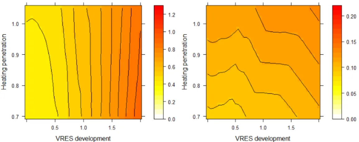
Figure 6: 95th percentile of normalised annual flexible power (left) and energy (right)
requirement in terms of VRES and electric heating penetrations
Figure 6 shows the annual flexibility requirements in terms of VRES and electric heating penetrations. VRES development is expressed in the same manner as for figure 5; an electric heating penetration of 1 corresponds to 2017 levels.
Save for low VRES penetration cases, reducing the penetration of electric heating barely has any impact on the annual flexible power requirement, the intermittent nature of wind being too much of a constraint. For high VRES cases, it even slightly increases the requirement. However, reducing electric heating penetration is beneficial where annual flexible energy is concerned and can compensate to some degree the increasing requirement caused by increased VRES penetrations.
As for electric cooling, it causes an insignificant decrease in annual flexi-bility requirement for very low VRES penetrations. There is too little electric cooling load in France for it’s penetration to have much of an impact in the foreseeable future.
3.3.2. Weekly flexibility requirement
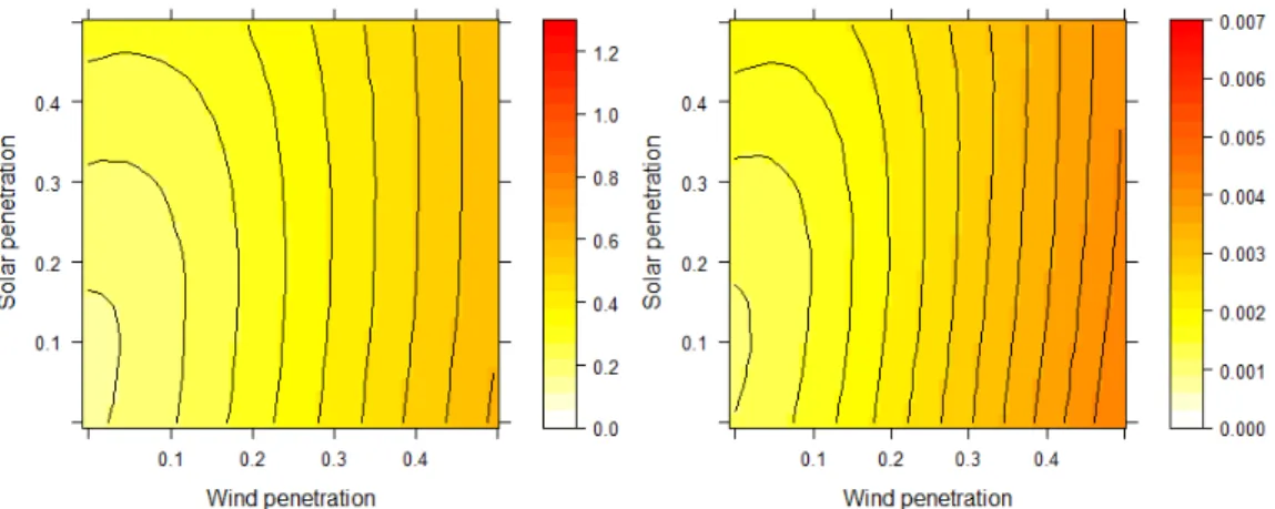
Figure 7 shows the 95th percentile of the need for weekly flexible power and energy observed in the French net load curve (F P R(w) and F ER(w)), expressed in terms of solar and wind penetrations. Electric heating and cooling were set to their 2017 value, interconnection was set to zero. As seen previously, the power requirement was normalised by the system’s maximum load (n.b. not net load), the energy requirement by the system’s average annual demand. Note that the scale for the flexible energy requirement is different from the one used in section 3.3.1.
Figure 7: 95th percentile of normalised weekly flexible power (left) and energy (right) requirement in terms of wind and solar penetrations
From a weekly perspective, if solar penetration has a slight impact for low wind penetrations, flexibility requirement is primarily a function of the share of wind in the electricity mix. It is interesting to note that the interac-tions between wind and solar are of the same nature for both flexible energy and flexible power requirements, contrary to the annual timescale. Intercon-nection development has a very limited impact for low VRES penetrations, but induces a notable requirement reduction in high VRES mixes.
Reduc-ing electric heatReduc-ing or increasReduc-ing electric coolReduc-ing penetrations has next to no impact.
The observations made in section 3.2 concerning the balance of requiments between different timescales partially hold. The flexible energy re-quirement remains 2 to 3 orders of magnitude smaller on the weekly timescale than the annual one. However, the dominating flexible power requirement can vary: network interconnection and electric heating penetration reduction having more impact on the annual requirement than the weekly one, even in France, when wind penetration is high, weekly flexible power requirement can be the most important.
3.3.3. Daily flexibility requirement
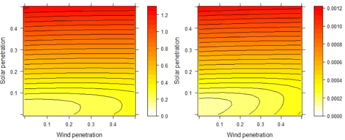
Figure 8 shows the 95th percentile of the need for daily flexible power and energy observed in the French net load curve (F P R(d) and F ER(d)), expressed in terms of solar and wind penetrations. Electric heating and cooling were set to their 2017 value, interconnection was set to zero. Note that the scale for the flexible energy requirement is different from the one used in sections 3.3.1 and 3.3.2.
Figure 8: 95th percentile of normalised daily flexible power (left) and energy (right) re-quirement in terms of wind and solar penetrations
From a daily perspective, solar generation and electricity demand are in phase, thus slightly reducing the flexibility requirements (both power and en-ergy), up to a certain threshold. Beyond that threshold, however, flexibility requirements are drastically increased (this phenomenon is well illustrated
by the famous "duck curve"). For high solar penetrations, the flexible power requirement is higher than what was observed for annual and weekly re-quirements, and higher even than Pmax (i.e. curtailment is required if load is not adapted). Wind penetration has somewhat of an effect for low solar penetrations, slightly increasing the daily flexibility requirements (more so for energy than power). Varying network interconnection, electric heating or cooling penetrations has next to no impact.
The threshold beyond which solar starts causing an increase in daily flex-ibility requirement varies with the considered country, it tends to occur at higher penetrations in southern European countries compared to northern European ones.
3.4. Prospective power system flexibility requirements
Figure 9 shows the distributions of normalised flexibility requirements in 2017 and in the Ampere Scenario in 2036 (see table 3). Results are evaluated on net load curves, network interconnections have been considered, electric heating and cooling penetrations in 2036 are set at 0.89 and 2.5 respectively (relative to values of 1 for 2017).
Figure 9: Flexibility requirements evaluated with I, pwind, psolar, pheat and pcool set at
2017 and Ampere scenario 2036 levels
Figure 10 shows the first order Sobol indices of I, pwind, psolar, pheat and pcool, for flexible power and energy requirements. The input variable values
were sampled in the interval [2017, Ampere 2036] using a uniform distri-bution. The sum of first order indices being very close to one, total Sobol indices have not been shown.
Figure 10: GSA results for flexible power (left) and flexible energy (right) requirements
Combining results from figures 9 and 10 with observations made in sec-tion 3.2, the following conclusions may be drawn regarding flexible power: (i) the annual flexible power requirement will slightly increase, the expected network interconnection development and heating penetration reduction be-ing insufficient to match the increase in requirement caused by wind (and to a much smaller degree, solar) power development, (ii) the weekly flexible power requirement will become very variable, its maximum will double un-der the sole influence of wind power development, exceeding the maximum annual requirement, (iii) the daily flexible power requirement will become very variable, its maximum will double almost entirely due to solar power development, reaching the current level of annual requirement.
If input variable values are sampled in the interval [Ampere 2036, 1.5 x Ampere 2036], GSA results are not particularly affected; if anything, the dependency of French flexible power requirements on VRES levels is further enhanced.
Similarly, the following conclusions may be drawn regarding flexible en-ergy: (i) the annual flexible energy requirement will slightly decrease,
ex-pected wind and network interconnection development and electric heating penetration reduction compensating the upward effect of solar power develop-ment, (ii) the weekly flexible energy requirement will become more variable, its maximum will double solely due to wind power development, but will remain about 25 times smaller than the annual requirement, (iii) the daily flexible power requirement will become more variable, its maximum will dou-ble due to VRES development, but will remain about 250 times smaller than the annual requirement.
GSA results for flexible energy requirement are slightly sensitive to the chosen boundaries. If input variable values are sampled between 1 and 1.5 times Ampere Scenario development in 2036, (i) network interconnection has an increased impact on the annual timescale, the impact of electric heating and wind power is reduced, (ii) network interconnection starts having a slight impact on the weekly timescale, (iii) solar power becomes the sole determi-nant on the daily timescale.
4. Conclusions
This paper presents a new set of frequency spectrum analysis based in-dicators quantifying annual, weekly and daily flexibility requirements, ex-panding the current metric paradigm which has concentrated on shorter timescales. The proposed methodology also allows the examination of these requirements’ sensitivity to five variables: the degree of network intercon-nection and the penetration of wind power, solar power, electric heating and cooling. These indicators have been applied to a case study, evaluating flexibility requirements for potential evolutions of the French power system, accounting for interconnection with electrically connected countries. A par-ticular focus was given to the 2017 situation and to an ambitious scenario for 2036.
The Global Sensitivity Analysis has shown that the most impacting vari-ables differ with the considered aspect of the flexibility problem. Both daily and weekly requirements are set to increase, the prior primarily due to solar power development, the latter almost exclusively due to wind power devel-opment. On the annual timescale, electric heating penetration reduction, wind power development and network interconnection should overcome the increasing effect of solar power where flexible energy is concerned. In terms of flexible power, wind power should drive the requirement up.
These conclusions are valid for France, they may change with location, depending on VRES penetrations, on the balance between wind and solar power and on the amount of electric heating. Several general conclusions can however be drawn: (i) flexible power requirements are of the same order of magnitude for annual, weekly and daily timescales, (ii) annual flexible energy requirements are greater than weekly and daily ones by one or two orders of magnitude, (iii) daily flexibility requirements are highly dependent on solar penetration, (iv) weekly flexibility requirements are highly dependent on wind penetration, and (v) annual flexibility requirements are a function of several factors.
The presented flexibility requirement quantification methodology and re-sults can be used by system operators to identify and understand future challenges, by flexibility providers to evaluate market potential for their so-lution and by policy makers to assess the implications of their decisions.
Having determined how and why flexibility requirement is likely to evolve under the influence of a set of long-term variables, the next step is to explore how the power system can adapt to its changing environment. The aim of ongoing work is to obtain an optimal combination of flexibility solutions, to see how this optimum is affected by the same set of long-term variables and to try and establish links between optimal combinations and sets of flexibility requirement. Solutions have a wide variety of characteristics and constraints, they will compete for a limited economic potential for each requirement, may have contradictory effects on different timescales or may have cascading effects: long-term levers could also provide short-term flexibility. The optimal flexibility mix must therefore be determined using a holistic approach, taking into consideration the entire energy system, different time horizons, on a wide geographical scale.
5. Acknowledgements
We would like to thank the anonymous reviewers for their valuable com-ments. Data for the research presented in this paper was provided by RTE, the French Transmission System Operator. Time series were derived by RTE on the basis of data produced by Météo-France, the French national meteo-rological service. This work is part of the OSMOSE project. It has received funding from the European Union’s Horizon 2020 research and innovation program under grant agreement n°773406. This article reflects only the au-thors’ views. The European Commission is not responsible for any use that
may be made of the information it contains. The European Commission was not involved in study design, data analysis or writing of this paper.
6. References References
[1] H. Holttinen, A. Tuohy, M. Milligan, E. Lannoye, V. Silva, S. Müller, L. Söder, et al., The flexibility workout: managing variable resources and assessing the need for power system modification, IEEE Power and Energy Magazine 11 (2013) 53–62.
[2] P. D. Lund, J. Lindgren, J. Mikkola, J. Salpakari, Review of energy system flexibility measures to enable high levels of variable renewable electricity, Renewable and Sustainable Energy Reviews 45 (2015) 785– 807.
[3] E. Lannoye, D. Flynn, M. O’Malley, Transmission, variable generation, and power system flexibility, IEEE Transactions on Power Systems 30 (2015) 57–66.
[4] M. Huber, D. Dimkova, T. Hamacher, Integration of wind and solar power in europe: Assessment of flexibility requirements, Energy 69 (2014) 236–246.
[5] T. A. Deetjen, J. D. Rhodes, M. E. Webber, The impacts of wind and solar on grid flexibility requirements in the electric reliability council of texas, Energy 123 (2017) 637–654.
[6] H. Kondziella, T. Bruckner, Flexibility requirements of renewable energy based electricity systems–a review of research results and methodologies, Renewable and Sustainable Energy Reviews 53 (2016) 10–22.
[7] E. Lannoye, D. Flynn, M. O’Malley, Power system flexibility assessment-state of the art, in: Power and Energy Society General Meeting, 2012 IEEE, IEEE, pp. 1–6.
[8] Y. V. Makarov, P. Du, M. C. Kintner-Meyer, C. Jin, H. F. Illian, Siz-ing energy storage to accommodate high penetration of variable energy resources, IEEE Transactions on Sustainable Energy 3 (2012) 34–40.
[9] E. Oh, S.-Y. Son, Energy-storage system sizing and operation strategies based on discrete fourier transform for reliable wind-power generation, Renewable Energy 116 (2018) 786–794.
[10] A. Belderbos, A. Virag, W. D’haeseleer, E. Delarue, Considerations on the need for electricity storage requirements: Power versus energy, Energy Conversion and Management 143 (2017) 137–149.
[11] F. Steinke, P. Wolfrum, C. Hoffmann, Grid vs. storage in a 100% re-newable europe, Rere-newable Energy 50 (2013) 826–832.
[12] N. Langrene, W. van Ackooij, F. Bréant, Dynamic constraints for aggre-gated units: Formulation and application, IEEE transactions on Power Systems 26 (2011) 1349–1356.
[13] A. Zerrahn, W.-P. Schill, Long-run power storage requirements for high shares of renewables: review and a new model, Renewable and Sustain-able Energy Reviews 79 (2017) 1518–1534.
[14] J. Ma, V. Silva, R. Belhomme, D. S. Kirschen, L. F. Ochoa, Evaluating and planning flexibility in sustainable power systems, in: Power and Energy Society General Meeting (PES), 2013 IEEE, IEEE, pp. 1–11. [15] NERC, Probabilistic Assessment Technical Guideline Document,
Tech-nical Report, North American Electric Reliability Corporation, 2016. [16] A. Tuohy, E. Lannoye, Metrics for Quantifying Flexibility in Power
System Planning, Technical Report, Electric Power Research Institute, 2014.
[17] H. Holttinen, J. Kiviluoma, A. Estanqueiro, T. Aigner, Y.-H. Wan, M. R. Milligan, Variability of load and net load in case of large scale dis-tributed wind power, in: 10th International Workshop on Large-Scale Integration of Wind Power into Power Systems as well as on Trans-mission Networks for Offshore Wind Power Farms, August 2010., pp. 853–861.
[18] S. Lumbreras, F. Banez-Chicharro, C. Pache, e-Highway 2050 - En-hanced methodology to define optimal grid architectures for 2050, Tech-nical Report, RTE, COMILLAS, ELIA, TU BERLIN, 2015.
[19] M. Fürsch, S. Hagspiel, C. Jägemann, S. Nagl, D. Lindenberger, E. Tröster, The role of grid extensions in a cost-efficient transforma-tion of the european electricity system until 2050, Applied Energy 104 (2013) 642–652.
[20] M. Kristiansen, M. Korpås, H. G. Svendsen, A generic framework for power system flexibility analysis using cooperative game theory, Applied Energy 212 (2018) 223–232.
[21] G. S. Eskeland, T. K. Mideksa, Electricity demand in a changing cli-mate, Mitigation and Adaptation Strategies for Global Change 15 (2010) 877–897.
[22] L. Wenz, A. Levermann, M. Auffhammer, North–south polarization of european electricity consumption under future warming, Proceedings of the National Academy of Sciences (2017) 201704339.
[23] M. Hekkenberg, R. Benders, H. Moll, A. S. Uiterkamp, Indications for a changing electricity demand pattern: The temperature dependence of electricity demand in the netherlands, Energy Policy 37 (2009) 1542– 1551.
[24] D. Quiggin, R. Buswell, The implications of heat electrification on na-tional electrical supply-demand balance under published 2050 energy scenarios, Energy 98 (2016) 253–270.
[25] N. Eyre, P. Baruah, Uncertainties in future energy demand in uk resi-dential heating, Energy Policy 87 (2015) 641–653.
[26] T. Boßmann, I. Staffell, The shape of future electricity demand: ex-ploring load curves in 2050s germany and britain, Energy 90 (2015) 1317–1333.
[27] Météo-France, CNRM, ARPEGE-Climate Version 5.2 Algorithmic Doc-umentation, 2011.
[28] M. Veysseire, S. Martinoni, S. Farges, Scénarios à climat constant, https://bit.ly/2qLSe0d, 2016.
[29] B. Delenne, C. De Montureux, M. Veysseire, S. Farges, Using weather scenarios for generation adequacy studies, https://bit.ly/2J5PTET, 2015.
[30] RTE, Bilan Prévisionnel de l’équilibre offre-demande d’électricité en France, Technical Report, RTE, 2017.
[31] E. Yukseltan, A. Yucekaya, A. H. Bilge, Forecasting electricity demand for turkey: Modeling periodic variations and demand segregation, Ap-plied Energy 193 (2017) 287–296.
[32] J. P. Barton, D. G. Infield, Energy storage and its use with intermittent renewable energy, IEEE transactions on energy conversion 19 (2004) 441–448.
[33] A. Mellit, M. Benghanem, S. A. Kalogirou, An adaptive wavelet-network model for forecasting daily total solar-radiation, Applied Energy 83 (2006) 705–722.
[34] S. Shamshirband, K. Mohammadi, H. Khorasanizadeh, L. Yee, M. Lee, D. Petković, E. Zalnezhad, Estimating the diffuse solar radiation using a coupled support vector machine–wavelet transform model, Renewable and Sustainable Energy Reviews 56 (2016) 428–435.
[35] A. Tascikaraoglu, B. M. Sanandaji, K. Poolla, P. Varaiya, Exploiting sparsity of interconnections in spatio-temporal wind speed forecasting using wavelet transform, Applied Energy 165 (2016) 735–747.
[36] M. M. Alam, S. Rehman, L. M. Al-Hadhrami, J. P. Meyer, Extraction of the inherent nature of wind speed using wavelets and fft, Energy for Sustainable Development 22 (2014) 34–47.
[37] T.-P. Chang, F.-J. Liu, H.-H. Ko, M.-C. Huang, Oscillation characteris-tic study of wind speed, global solar radiation and air temperature using wavelet analysis, Applied energy 190 (2017) 650–657.
[38] I. M. Sobol, Global sensitivity indices for nonlinear mathematical mod-els and their monte carlo estimates, Mathematics and computers in simulation 55 (2001) 271–280.
[39] A. Bossavy, R. Girard, G. Kariniotakis, Sensitivity analysis in the tech-nical potential assessment of onshore wind and ground solar photovoltaic power resources at regional scale, Applied Energy 182 (2016) 145–153.
[40] M. Lacirignola, P. Blanc, R. Girard, P. Perez-Lopez, I. Blanc, Lca of emerging technologies: addressing high uncertainty on inputs’ variabil-ity when performing global sensitivvariabil-ity analysis, Science of the Total Environment 578 (2017) 268–280.
[41] G. Mavromatidis, K. Orehounig, J. Carmeliet, Uncertainty and global sensitivity analysis for the optimal design of distributed energy systems, Applied Energy 214 (2018) 219–238.
[42] A. Rogeau, R. Girard, G. Kariniotakis, A generic gis-based method for small pumped hydro energy storage (phes) potential evaluation at large scale, Applied Energy 197 (2017) 241–253.
[43] R. Silva, M. Pérez, M. Berenguel, L. Valenzuela, E. Zarza, Uncertainty and global sensitivity analysis in the design of parabolic-trough direct steam generation plants for process heat applications, Applied Energy 121 (2014) 233–244.
[44] A. Saltelli, M. Ratto, T. Andres, F. Campolongo, J. Cariboni, D. Gatelli, M. Saisana, S. Tarantola, Global sensitivity analysis: the primer, John Wiley & Sons, 2008.
[45] A. Saltelli, P. Annoni, How to avoid a perfunctory sensitivity analysis, Environmental Modelling & Software 25 (2010) 1508–1517.